Estimation of the Fracture Toughness Threshold of a Ferritic Steel at the Lower Ductile to
Brittle Transition Region
Carlos Berejnoia*, Santiago Vaccab, Claudia Galarzaa, Juan Elías Perez Ipiñac,d
Received: August 31, 2015; Revised: March 23, 2016; Accepted: July 28, 2016
The ADN420 ferritic steel (A615 steel Grade 60 [420]), used as reinforcing bars (rebar) in concrete, shows the so called ductile to brittle transition. Room temperature is located on the lower third region of the transition zone. In this work, the fracture toughness of this steel working at room temperature was studied statistically. For such a purpose, 125 compact test specimens were machined from commercial bars and tested at room temperature to determine the Jc and KJc critical fracture toughness values. Several continuous probability functions with threshold parameter were adjusted to the J and K datasets.
Keywords: ferritic steels, fracture toughness, scatter, threshold, weakest link
* e-mail: [email protected]
1. Introduction
The fracture toughness of materials working at the ductile to brittle transition usually shows considerable scatter1-8. It is believed that the relative position of
the crack tip related to microstructural heterogeneities causes the scatter, this theory is known as the weakest link theory2-4. In this case, the resulting statistical
distribution characterizes the fracture toughness of the tested specimens. From a fracture mechanics point of view, the material will be as reliable as that point with the worst possible microstructural heterogeneity relative to the crack tip. Thus, the fracture toughness corresponding to this worst situation, which can be characterized by a threshold parameter of the statistical distribution, becomes a technologically interesting parameter. Further, it is considered as thickness independent, since a thicker test piece will only increase the chances of having the most unfavorable microstructural heterogeneity relative to the crack tip; afecting scatter, but not the threshold value, being this a material property. Validating this theory presents the diiculty that the sample sizes required to statistically characterize a material for diferent temperatures and thicknesses makes it economically impractical.
Experimental data may be itted by means of diferent statistical functions. If one statistical distribution function is known to be correct for certain physical or characteristic property, then it is possible to estimate all the parameters for such a distribution. In this way, the minimum toughness
of a material could be estimated as a threshold parameter or the value for a probability failure level of the statistical distribution.
For the fracture toughness characterization of ferritic steels in the ductile to brittle transition zone, it is quite common to calculate the J integral and then convert the results to the stress intensity factor K (Eq. (1)).
a Facultad de Ingeniería, Consejo de Investigación de la Universidad Nacional de Salta – CIUNSa,
Universidad Nacional de Salta, Avda. Bolivia 5500, Salta, Argentina
b Facultad Ingeniería, Instituto de Ensayo de Materiales, Universidad de la República, Montevideo,
Uruguay
c Grupo Mecánica de Fractura, Universidad Nacional del Comahue, Neuquén, Argentina
d Consejo Nacional de Investigaciones Cientíicas y Técnicas – CONICET, Neuquén, Argentina
( ) K v EJ 1 1 Jc C 2
= Q - V
ν is the Poisson coeicient (0.3) and E the Young modulus (210 GPa).
The results are adjusted mostly with a two parameter Weibull distribution (2P-W)1,3,9-13, Eq. (2), or with a three
parameter WeibullI distribution (3P-W)2,4,14,15, Eq. (3), both
in terms of JC or KJc.
( ) exp exp P J Jc P K K 1 2 1 b Jc b 0 0 J K = - -= - -T T Y Y # # & & ( ) exp exp P J J Jc J P K K K K 1 3 1 min min min min b Jc b 0 0 J K = - - - -= - - - -T T Y Y # # & &
The standard ASTM E1921-158 indicates the statistical
treatment of K values derived from J results for 1’’ compact specimen (1T-CT), with the use of a 3P-W distribution, considering two of the parameters as ixed (Eq. (4)).
( ) exp
P
K K
1 Jc 2020 4
0 4
= - #-T -- Y&
Other statistical functions may be used, such as the log-normal and some exponential based distributions16.
The ADN 420 steel, equivalent to the A615 steel Grade 6017, is used as reinforcing bars for concrete. On the material
designation, “ADN” stands for “naturally hardened steel” in Spanish and “420” for minimum yield strength of 420 MPa. For this steel, room temperature corresponds to the lower third of the ductile-to-brittle transition region.
A large set, from a fracture toughness tests point of view, of AND 420 specimens was tested in this work in order to assure it was representative of the population. Threshold parameters were estimated using different statistical distributions and then compared.
2. Material and methods
2.1. Fracture toughness tests
The critical fracture toughness (JC) of the ADN 420 steel was determined by testing compact specimens (C(T)) at 20 °C, according to the ASTM 1820-13e1 standard18.
This material is produced as cylindrical bars by continuous casting, and then hot rolled to diferent inal diameters (38 mm bars were used in this work).
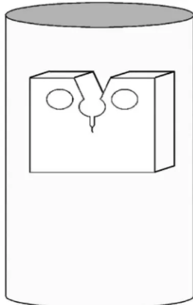
A total of 126 C(T) specimens were machined to a width of 25 mm and a thickness of 12.5 mm with the crack in the R-L orientation according to ASTM E1823-1319 (Figure 1).
The specimens where pre-cracked in a displacement controlled fatigue test machine.
The specimens where tested in a 100 KN Amsler screw testing machine. Tests were quasi-static, loading rate was 1 MPa.m1/2. Force (P) was measured with a 20 kN load cell
and displacements (v) with a clip-gage mounted at the knife edges of the specimens, which were collinear to the load line. Measurements were digitally recorded to a PC. Tested specimens were cooled to -20 °C and then fractured in the Amsler testing machine.
Jc values were calculated according to ASTM E1820-13e118 from the P vs. v records and specimen dimensions,
then they were converted into KJc values by means of Eq. (1).
2.2. Statistical Analysis
Two datasets were obtained with the procedure described above, one for Jc and one for KJc. Several continuous
non-Figure 1: Specimen extraction scheme.
negative distributions, most of them with a threshold parameter, were adjusted to both datasets using Easyit Software20:
• Functions that includes exponential: Chi-Squared (2P), Erlang (3P), Exponential (2P), Frechet (3P), Gamma (3P), Gen. Gamma (4P), Inv. Gaussian (3P), Levy (2P), Lognormal (3P), Pearson 5 (3P), Rayleigh (2P), Weibull (3P).
• Functions not including exponencial: Burr (4P), Dagum (4P), Fatigue Life (3P), Log-Logistic (3P), Pareto, Pearson 6 (4P).
A number followed by the letter P (in parentheses) indicates the number of parameters used in each distribution, in cases where diferent number of parameters could be used. For instance, Weibull (3P) responds to Eq. (3), while Eq. (2) would be used for Weibull (2P).
According to Wallin16, exponential distributions (such
as Weibull, Gumbel and Log-Normal) describe fracture toughness results better than the Normal distribution. In this work, the Gumbel function was not included because it has not a threshold parameter; it is an unbounded distribution, like the Normal one, with a range of (–ininity, ininity).
3. Results and Discussion
From the 126 specimens machined, only 117 tests resulted geometrically valid.
The obtained Jc and KJc values are presented in Table 1. The minimum and maximum measured Jc values were 12.55 and 43.63 N/mm respectively; and their equivalent KJc were
53.43 and 99.63 MPam½ respectively. Because the tests
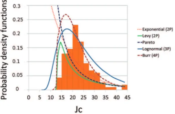
were performed in the lower third of the transition region, all 117 specimens failed by cleavage without previous stable crack growth giving valid results (Jlimit=175 N/mm; KJc(limit)=200.96 MPa.m0.5). Figure 2 and Figure 3 show the
histograms of the datasets for Jc, while the corresponding histograms for KJc are shown in Figure 4 and Figure 5. The continuous curves that result from multiplying the probability density functions by the intervals width are also shown in these igures. The discrimination in good or bad itting was supported by the Anderson-Darling test (also performed with Easyit Software20).
Dagum (4P) does not adjust the datasets at all, being impossible to present the distribution in the scale of Figures 2 to 5.
The threshold parameters for the adjusted distributions are shown in Figure 6 and Figure 7, for the Jc and KJc datasets respectively. In the igures, the distributions are ordered from the worst itting (left) to the best adjustment (right), according to how close is the estimated threshold parameter to the experimental minimum. Also, the values Jmin=11 N/ mm and Kmin=50 MPa.m1/2 are included in the igures as
horizontal lines and they were used as acceptable values for threshold estimation. Figure 7 also shows the threshold imposed in ASTM E1921-15, Kmin=20 MPa.m1/2.
The exponential type Frechet (3p) distribution is not included in Figure 6 and Figure 7 because the threshold parameter estimated for this sample resulted negative, around of -108.
According to Figure 6 and Figure 7, Rayleigh (2P), Weibull (3P), Exponencial (2P), Pareto and Levy (2P) are the distributions that present thresholds nearer to the ninimum experimental. Exponencial (2P), Levy (2P) and Pareto do not adjust the
Table 1: Datasets for Jc and KJc valid according to the ASTM 1820-13e1 standard.
Jc [N/mm] KJc [MPa.m½]
17.08 20.00 18.79 37.40 62.78 67.94 65.85 92.90
20.84 24.26 31.71 18.93 69.35 74.82 85.54 66.09
17.21 15.26 22.07 39.56 63.02 59.34 71.37 95.55
29.62 24.41 22.73 16.97 82.68 75.05 72.43 62.58
28.20 13.04 23.88 26.65 80.67 54.86 74.23 78.42
30.32 18.30 23.07 14.41 83.65 64.99 72.96 57.67
21.42 32.42 16.27 33.83 70.31 86.50 61.27 88.36
16.83 20.91 24.93 22.79 62.32 69.46 75.85 72.52
33.01 19.69 18.97 21.41 87.28 67.41 66.16 70.29
14.95 15.23 21.12 28.36 58.74 59.28 69.81 80.90
29.76 17.02 27.17 22.87 82.87 62.67 79.18 72.65
17.13 20.71 22.29 29.01 62.87 69.13 71.72 81.82
24.03 16.72 20.64 27.48 74.47 62.12 69.02 79.63
32.49 29.55 21.51 25.33 86.59 82.58 70.45 76.46
17.79 22.17 23.22 22.33 64.07 71.53 73.20 71.78
22.86 18.09 22.38 26.28 72.63 64.61 71.87 77.88
22.00 43.63 28.06 17.87 71.25 100.34 80.47 64.22
21.65 18.53 21.70 21.81 70.68 65.39 70.77 70.94
16.46 25.04 19.46 23.67 61.63 76.02 67.01 73.91
21.34 23.38 20.42 16.62 70.18 73.45 68.65 61.93
23.16 20.49 26.31 21.56 73.11 68.76 77.92 70.54
26.03 30.52 19.72 27.26 77.50 83.92 67.46 79.31
23.21 33.52 22.33 18.44 73.19 87.95 71.78 65.23
27.61 22.64 21.10 22.18 79.82 72.28 69.78 71.54
15.88 17.76 23.94 18.27 60.54 64.02 74.33 64.93
26.20 25.95 22.10 18.42 77.76 77.39 71.41 65.20
31.11 15.78 43.50 20.95 84.73 60.35 100.19 69.53
19.62 12.55 22.62 67.29 53.82 72.25
24.14 13.28 30.94 74.64 55.36 84.50
Figure 2: Histogram and scaled probability density functions. Good ittings for Jc results.
Figure 3: Histogram and scaled probability density functions. Bad
ittings for Jc results.
Figure 4: Histogram and scaled probability density functions. Good
ittings for KJc results.
Figure 5: Histogram and scaled probability density functions. Bad
ittings for KJc results.
Figure 6: Threshold parameters for the adjusted distributions to
the Jc dataset.
Figure 7: Threshold parameters for the adjusted distributions to
the KJc dataset.
histograms neither in Jc nor in KJc (Figure 3 and Figure 5). It is also seen that the 3PW distribution adjusts fairly to both Jc and KJc datasets while giving a high threshold parameter, lower than the minimum experimental and close to it.
Special attention was paid to Rayleigh (2P) distribution (Eq. (5)). The scale and threshold parameters are μ and γ, respectively.
( )
P 1 e 21 5
2
\ = - v
\ c
-
-Q
V
T YThe original Weibull distribution was presented by Weibull21, where he stated that the appropriate mathematical
expression for a weakest link model has the form shown in Eq. (6)
( )
P
1
e
n6
\
= -
-{ \Q
V
QVIn Eq. (6), n is the number of links in the chain. Weibull also exposed that the simplest expression for the function φ (x) is:
( )7
u m 0 { \ \ \ \ =
-Q
V
Q
V
Equations (8) and (9) are two proposed distributions2,4,
related to the weakest link model, but applied to fracture toughness characterization.
( )
P J 1 e B 8
B J J J J min min N b 1 0 = - - -
-Q V T Y
( )
P K 1 e B 9
B K K KK min minb 0 0 = - - -
-Q V T Y
BN/B1 and B/B0 refer to a ratio size, being factors that take into account the probability of inding a diferent number of initiators cleavage sites in the crack tip. More initiators are found when this factors are greater than one, as the specimen size is greater.
The Rayleigh (2P) distribution presented in Eq. (5) can be considered as a particular case of the Weibull distribution, with
n equal to 1/2 and the shape parameter equal to 2, resulting:
( )10
2
{ \ n
\ c
=
-Q V T Y
The advantage implicit in Eqs. (8) and (9) is their use for adjusting distributions for samples of specimens of diferent sizes. For instance, one may estimate the shape parameter for datasets of B1 or B0 sizes (Eq. (3)), and then using Eq. (8) or (9) the datasets of B or BN thicknesses would be adjusted. The factors BN/B1 and B/B0 would be the number n of links in the chain presented by Weibull.
So, Eqs. (5), (8) and (9) are all mathematical expressions that respond to Weibull distribution. The main diference is that Eq. (5) considers as ixed the shape parameter, and no variation of size ratio is allowed, because it is ixed.
The statistical distribution imposed in ASTM E1921-158 for the determination of the T
0 reference temperature
(Eq. (4)) is similar to Rayleigh distribution, in the sense that the shape parameter is ixed (b=4), although it permits
the variation of size ratio. This distribution is applicable to datasets of specimens of 1”, no factor B/B0 is included because the results for diferent sizes must be converted previously to 1” thickness.
4. Conclusions
Jc values showed signiicant scatter for the AND420 steel at 20 °C and 12.5 mm thickness. The three parameter Weibull distribution adjusted well to data on both Jc and KJc parameters. This function presented a high threshold parameter compared to the other distributions analyzed.
The Rayleigh distribution presents a good adjustment for this sample. This function is a particular case of Weibull distribution (with shape parameter equal to 2). Further research must be performed in the direction of the convenience of Rayleigh distribution compared to the traditional Weibull function, using diferent samples sizes, and diferent materials.
5. Acknowledgements
To Consejo Nacional de Investigaciones Cientíicas y Tecnológicas (CONICET) and to Consejo de Investigación de la Universidad Nacional de Salta (CIUNSa) by the support to this work.
6. References
1. Landes JD, Shafer DH. Statistical Characterization of Fracture in the Transition Region. ASTM STP 700. West Conshohocken: ASTM International; 1980. p. 368-382.
2. Landes JD, McCabe DE. The Efect of Section Size on the Transition
Temperature of Structural Steels. West Conshohocken: ASTM International; 1984.
3. Wallin K. The scatter in KIC-results. Engineering Fracture
Mechanics.1984;19(6):1085-1093.
4. Wallin K. Statistical aspects of constraint with emphasis on testing and analysis of laboratory specimens in the transition region. In: Hackett EM, Schwalbe KH, Dodds RH, eds. Constraint Efects in Fracture STP 1171. West Conshohocken: ASTM International; 1993. p. 264-288.
5. Heerens J, Hellmann D. Development of the Euro fracture toughness dataset. Engineering Fracture Mechanics. 2002;69(4):421-449.
6. Larrainzar C, Berejnoi C, Perez Ipiña JE. Comparison of 3P-Weibull parameters based on JC and KJC values. Fatigue & Fracture of Engineering Materials & Structures. 2010;34(6):408-422.
7. Perez Ipiña JE, Berejnoi C. Experimental Validation of the Relationship Between Parameters of 3P-Weibull Distributions Based in Jc or KJC. In: 13th International Conference on Fracture;
2013 June 16-21; Beijing, China.
8. ASTM E1921-15ae1. Standard Test Method for Determination of
9. Iwadate T, Tanaka Y, Ono S, Watanabe J. An Analysis of Elastic-Plastic Fracture Toughness Behavior for JIc Measurement in the Transition Region. West Conshohocken: ASTM International; 1983. p. 531-561.
10. Anderson TL, Stienstra D, Dodds RH. A Theoretical Framework
for Addressing Fracture in the Ductile-Brittle Transition Region. West Conshohocken: ASTM International; 1994. p. 186-214.
11. Landes JD, Zerbst U, Heerens J, Petrovski B, Schwalbe KH.
Single-Specimen Test Analysis to Determine Lower-Bound Toughness in the Transition. West Conshohocken: ASTM International; 1994. p. 171-185.
12. Heerens J, Zerbst U, Schwalbe KH. Strategy for Characterizing Fracture Toughness in the Ductile to Brittle Transition Regime. Fatigue & Fracture of Engineering Materials & Structures. 1993;16(11):1213-1230.
13. Heerens J, Pfuf M, Hellmann D, Zerbst U. The lower bound toughness procedure applied to the Euro fracture toughness dataset. Engineering Fracture Mechanics. 2002;69(4):483-495.
14. Neville DJ, Knott JF. Statistical distributions of toughness and fracture stress for homogeneous and inhomogeneous materials.
Journal of The Mechanics and Physics of Solids.1986;34(3):243-291.
15. Perez Ipiña JE, Centurion SMC, Asta EP. Minimum number of specimens to characterize fracture toughness in the ductile-to-brittle transition region. Engineering Fracture Mechanics. 1994;47(3):457-463.
16. Wallin K. Fracture toughness of engineering materials - estimation and application. Warrington: EMAS publishing; 2011.
17. ASTM A615 / A615M - 15a. Standard Speciication for Deformed
and Plain Carbon-Steel Bars for Concrete Reinforcement. West Conshohocken: ASTM International; 2015.
18. ASTM E1820 - 13e1. Standard Test Method for Measurement of
Fracture Toughness. West Conshohocken: ASTM International; 2013.
19. ASTM E1823 - 13. Standard Terminology Relating to Fatigue and
Fracture Testing. West Conshohocken: ASTM International; 2013. 20. Mathwave. EasyFit - software. Available from: <http://www.
mathwave.com>. Access in: 18/02/2015.