ISSN 0104-6632 Printed in Brazil
www.abeq.org.br/bjche
Vol. 22, No. 01, pp. 105 - 116, January - March, 2005
Brazilian Journal
of Chemical
Engineering
FRONT TRACKING IN RECIRCULATING FLOWS:
A COMPARISON BETWEEN THE TVD AND RCM
METHODS IN SOLVING THE VOF EQUATION
L. F. Lopes Silva, C. E. Fontes and P. L. C. Lage
*Programa de Engenharia Química, COPPE, Universidade Federal do Rio de Janeiro (UFRJ), Phone: +(55) (21) 2562-8304, Fax: +(55) (21) 2562-8300,
PO Box 68502, ZIP Code 21945-970 Rio de Janeiro - RJ, Brazil. E-mail: [email protected]
(Received: February 8, 2003 ; Accepted: August 12, 2004)
Abstract - The modeling and simulation of mold filling must include a method to capture the interface formed between the inlet fluid and the fluid that was initially in the mold. A commonly used front-capturing method in a Eulerian mesh is the volume-of-fluid (VOF) method. The VOF advection equation solution may show numerical diffusion and/or dispersion and high-order numerical schemes, such as the TVD schemes with dimensional splitting, have to be employed to discretize the convective terms. The present contribution explores the use of RCM for solution of the VOF color-function equation during mold filling with recirculating flows. The Navier-Stokes equations are solved by a finite-volume method using the SIMPLER algorithm. Filling simulations using the TVD and RCM methods are compared. RCM was able to generate diffusion-free results, sharply defining the interface, even when topological changes (generation of droplets) occur.
Keywords: Interface capturing; Mold filling; RCM; TVD schemes; VOF schemes; Computational fluid dynamics.
INTRODUCTION
A variety of industrial processes include a step of filling some kind of cavity (thermoplastic injection molding, reaction injection molding, casting of metal pieces, food extrusion processes, etc). The design of these cavities involves a very expensive trial-and-error procedure in order to avoid filling problems, like heterogeneity in the final piece or air entrapment. This is especially true in the polymer industry. Due to this fact, during the last two decades many researchers have been developing computational methods that allow simulation of cavity filling, which shortens the expensive empirical stage. One of the most challenging problems in constructing a successful simulator is how to capture and track the interface formed
between the inlet fluid and the fluid that was initially inside the cavity.
presented and compared: the use of a high-order TVD scheme (total variation diminishing) developed by Chakravarthy and Osher (1985) and the use of a RCM scheme (random choice method) adapted from Toro (1999). Both schemes use dimensional splitting.
TVD methods are one of the most significant achievements in the development of numerical methods for partial differential equations in the last 20 years or so, although the preliminary ideas can be traced as far back as 1959 to the pioneering work of Godunov, continued later by van Leer. In 1965, Glimm introduced RCM and Colella (1982) contributed to developing and increasing knowledge of the method, considering its advantages and limitations.
In this work, the effectiveness of TVD and RCM for cavity-filling simulation are compared for both nonrecirculating and recirculating flows. In the filling, it is assumed that both fluids had the same properties. Thus, the pressure and velocity fields could be obtained for the steady-state flow throughout any cavity and then used for the filling simulation with both methods. This eliminates any flow field disturbance that would arise in a filling simulation for unsteady fluid flow. These steady-state flow solutions are obtained by solving the transient mass and momentum conservation equations using a finite-volume method and the SIMPLER algorithm until the steady-state flow reached a given tolerance. The effects of surface tension at the interface are not included in the analysis.
FLUID DYNAMICS EQUATIONS
The 2D-Cartesian mass and momentum conservation equations for a Newtonian fluid with constant density and viscosity, used in the simulation of flow through 2D-cavities, are presented below in a dimensionless form.
( )
( )
( )
ref ref
U V
Re Re 0
X Y
∂ ϕ ∂ ϕ ∂ ϕ
+ + =
∂τ ∂ ∂ (1)
( )
(
)
(
)
ref ref
yx xx ref
U UU VU
Re Re X Y T T P Re
X X Y
∂ ϕ ∂ ϕ ∂ ϕ
+ + = −
∂τ ∂ ∂
∂ ∂ ∂ − − + ∂ ∂ ∂ (2)
( )
(
)
(
)
ref ref xy yy refV UV VV
Re Re
X Y
T T
P Re
Y X Y
∂ ϕ ∂ ϕ ∂ ϕ
+ + = −
∂τ ∂ ∂
∂ ∂ ∂ − − + ∂ ∂ ∂ (3) xx
U 2 U V
T 2
X 3 X Y
∂ ∂ ∂
= − Γ + Γ +
∂ ∂ ∂ (4)
yx xy U V T T Y X ∂ ∂
= = −Γ +
∂ ∂
(5)
yy V 2 U V
T 2
Y 3 X Y
∂ ∂ ∂
= − Γ + Γ +
∂ ∂ ∂ (6)
where in in med med x y X Y D D u v U V v v = = = = (7) y x 2 med
p g y g x
P
v
− ρ − ρ = ρ ref 2 ref in t D µ τ =
ρ (8)
in med ref ref
ref ref
ref D v
Re = ρ Γ = µ
µ µ
ρ ϕ =
ρ
(9)
and t is the time; x and y are the spatial coordinates;
ρ is the density; µ is the viscosity; ν is the kinematic viscosity; u and v are the velocity components in x and y directions, respectively; p is the pressure; gi is
the body force in i direction; Din is the inlet width
and vmed is the mean inlet velocity. The subscript ref
refers to the inlet fluid properties.
After applying a finite-volume discretization on a staggered grid using the power-law scheme, the steady-state solution is achieved using the SIMPLER scheme (Patankar, 1980). The numerical code has been tested against benchmark results for the backward facing step flow (Gartling, 1990) with good agreement (Fontes et al., 1999).
tolerance assumes a very small value, the relative tolerance controls the convergence criterion. Absolute and relative tolerances of 10-6 for the
velocity components and of 10-5 for the pressure
were used. The criterion used to assume that the steady state was achieved was the same mixed tolerance criterion described above, but using absolute and relative tolerances of 10-4 for all the
variables in every control volume between two consecutive times.
VOF-TVD SCHEME
The volume-of-fluid (VOF) method is an interface-capturing method (Ferziger & Pèric, 1997). The fluids on both sides of the interface are marked by either massless particles or an indicator (color) function. In the VOF method the advection of the color function F, given by Equation (10) in dimensionless form, has to be solved. The F field values are stored at in the staggered finite-volume grid similarly to the pressure field.
F F F
Re U ReV 0
X Y
∂ + ∂ + ∂ =
∂τ ∂ ∂ (10)
As seen above, U and V are known from the steady-state solution. The simulated physical situation corresponds to the steady flow of a fluid through the cavity that suddenly becomes colored and starts to displace the colorless one. Obviously, if the physical property remains the same, so do the velocity and the pressure fields. For a given volume, F is equal to 0 when the volume has no colored fluid, but it is equal to 1 when the volume is completely filled with colored fluid. The interface has F values between 0 and 1.
Typical problems associated with the solution of hyperbolic equations like Equation (10) (numerical diffusion and dispersion) are reduced by the use of a total variation diminishing (TVD) scheme. Good summaries of TVD schemes are given by Sweby (1984) and Toro (1999). A numerical method is TVD if Equation (11), where ξ is the transported variable and TV(ξ) is its total variation, is valid for scalar conservation laws.
( ) ( )
( )
n 1 n
i i 1
i
TV TV ,
where
TV
+
−
ξ ≤ ξ
ξ =
∑
ξ − ξ(11)
Chakravarthy and Osher (1985) described one-dimensional second and third-order accurate TVD schemes with low truncation errors. These schemes were used to solve advective equations, like Equation (10). Goodman and LeVeque (1985) proved that there is no multidimensional TVD scheme, but Chakravarthy and Osher (1985) showed extremely good numerical results using their scheme. Based on its simplicity and good results, the Chakravarthy and Osher (1985) third-order scheme is used in the present work. In order to try to keep the TVD characteristics of the 1-D scheme, a dimensional splitting is applied during the numerical solution of Equation (10). Therefore, the explicit discretized form of Equation (10), with dimensional splitting, is given by Equations (12) and (13), where
1 / 2 / 2
∆τ = ∆τ . The splitting algorithm, in
accordance with Toro (1999), is described below. i) For each time step ∆τ, integrate first in X direction up to ∆τ1/2 using Eq. (12).
ii) Then, using F1/2, integrate in the Y direction up to
∆τ by Eq. (12), determining F.
iii)In order to achieve second-order accuracy for every-other time step, invert the X and Y integrations in the next time step ∆τ.
(
o o)
P e w
1 / 2 o 1 / 2
P P
U F F
F F Re
X
−
= − ∆τ
∆ (12)
(
1 / 2 1/ 2)
P n s
1/ 2
P AUX
V F F
F F Re
Y
−
= − ∆τ
∆ (13)
The F fluxes at the faces of the volumes are determined using the upwind-TVD scheme. For example, for the east face, for each j line, the flux is given by Eqs. (14) to (21). In these equations the index P stands for position (i, j) , E for position(i 1, j)+ , e for position (i 1 2, j)+ , ee for position (i 3 2, j)+ , w for position (i 1 2, j)− , n for position (i, j 1 2)+ and s for position (i, j 1 2)− . When γ equals 1/3 and β equals 4 these equations correspond to a third-order upwind scheme. Equation (14) represents the flux given for the Engquist-Osher first-order scheme (Osher & Chakravarthy, 1984). The minmod function is defined by Equation (19) and it is used to define the limited fluxes given in Equations (17) and (18). The fluxes for the other faces are obtained by changes in subscripts.
P e i 1 e e
i 2
U F U F f h
+
[
]
[
]
e 1 i i i i 1
i 2
f f max 0, U F max 0, U F+
+
= = − − (15)
e e w e w
e ee e ee
1
h d d d d
4
1
d d d d
4
+ +
+ +
− − − −
= φ + φ + γ φ − φ −
− φ + φ + γ φ − φ
(16) e w e w e w
d minmod(d , d )
d minmod(d , d )
+ + +
+ + +
φ = φ β φ
φ = φ β φ
(17)
e ee
e
ee e
ee
d minmod(d , d )
d minmod(d , d )
− − −
− − −
φ = φ β φ
φ = φ β φ
(18)
( )
( )
( )
{
}
minmod a,b sign a
max 0,min a ,bsign a
= (19)
(
)
1 2e i i i 1 i
dφ = φ+ d ++ =U F+ −F , Ui > 0 (20)
(
)
1 2
e i i i 1 i
dφ = φ− d −+ =U F+ −F , Ui≤ 0 (21)
Osher and Chakravarthy (1984) prove that their scheme is stable only for the Courant number, given by Eq. (22) for both X and Y directions, equal to or less than 0.4.
X
Y
u t U
C Re and
x X
v t V
C Re y Y ∆ ∆τ = = ∆ ∆ ∆ ∆τ = = ∆ ∆ (22)
Boundary conditions for this equation are as follows: the cells outside the mold inlet are considered to be completely filled with colored fluid (F = 1), all cells outside the mold at the outlet are considered to be completely filled with colorless fluid (F = 0) and there is no F flux at the other boundaries. At the beginning of the filling process, the mold is filled with colorless fluid (F = 0).
VOF-RCM SCHEME
Glimm (1965) introduced the random choice method but it was Colella (1982) who really developed this numerical method, discussing its advantages and limitations. Essentially, RCM is applicable to scalar problems in any number of dimensions without loosing its capacity to maintain the perfect resolution of contact discontinuities with no diffusion or dispersion. As F in Equation (10) is a scalar variable, RCM perfectly matches the necessities of the VOF method. Silva and Lage (2001) show a successful 1-D application of this scheme.
RCM chooses randomly among possible solutions of local Riemann problems associated with the dimensional splitting of Equation (10). The method used in this work is one given by Toro (1999) for a staggered grid in which a local 1-D Riemann problem is solved twice for each direction at each integration step: once between τn and τn+1/2 and once
between τn+1/2 and τn+1. It is exactly because RCM
solves the local Riemann problem that it does not show numerical diffusion. RCM stability is also dependent on the local Courant number, given by Equation (22). For the RCM used in this work, both Courant numbers have to be equal to or less than 1.
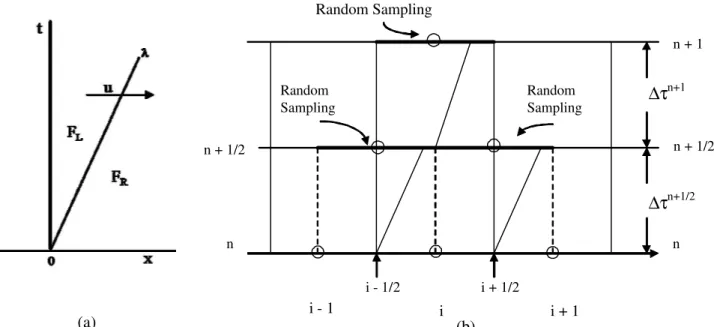
The local Riemann problem for Eq. (10) uses the local states (FL and FR) around the interface between
two control volumes. The exact solution of the local 1-D Riemann problem is shown in Fig. 1-a. It consists in a single contact discontinuity propagation from the origin with velocity u and slope λ = 1/u. Naturally, the solution values are equal to FL on the
left of the straight line with slope λ = 1/u and equal to FR on the right.
In order to explain this method, let’s consider its application to the integration of the F value in a given 1-D volume i of a uniform mesh in the X direction, as illustrated in Fig. 1-b, for a time step ∆τ. First, the local 1-D Riemann problems are solved at both volume interfaces in the first half-time step,
n 1 / 2+ n 2
∆τ = ∆τ . At interface
(
i 1 2−)
, thediscontinuity propagates a distance
i 1 2 X,i 1 2
d X= − +C + ∆X 2 during ∆τn 1 / 2+ . The position r X= i 1 2− + θ ∆n X is sampled by a random number θn ∈ [0,1]. If r ≤ d, then n 1 2 n
i 1 i 1 2
number θn to obtain n 1 2 i 1 2 ˆF +
+ . Then, another random
number θn+1 is generated, and a similar procedure is
applied to obtain the solution for volume i at the end of the time interval, Fin 1+ . Thus, two new random numbers are generated for each time step and for each direction. The complete algorithm can be described as follows:
i) Solve the Riemann problems RP F , F
(
i 1n− in)
and(
n n)
i i 1
RP F ,F+ to find solutions ˆFi 1 2n 1 2−+ and ˆFi 1 2n 1 2++ ; ii) For the first half-time step ∆τn 1 / 2+ , random sample these solutions based on random number θn:
( )
n 1 2 n 1 2 n i 1 2 ˆi 1 2F−+ =F−+ θ and Fi 1 2n 1 2++ =Fˆi 1 2n 1 2++
( )
θn ;iii) Solve Riemann problem RP F
(
i 1 2n 1 2−+ ,Fi 1 2n 1 2++)
tofind solution ˆFin 1+ ;
iv)For the second half-time step ∆τn 1 / 2+ , random sample this solution based on a new random number
n 1+
θ : Fin 1+ =Fˆin 1+
( )
θn .The same dimensional splitting applied in the VOF-TVD scheme is applied in the VOF-RCM scheme, which uses twice the 1-D scheme just described. As RCM is intrinsically a statistical scheme, front behavior may vary between simulation runs for the same problem, which introduces some uncertainty regarding the actual position of the fluid interface. Due to this statistical nature, uncertainty at the fluid interface decreases as the grid is refined. This occurs because more random numbers are generated to obtain the solution at a given time due to the Courant number limitations. The random number generator used was the IMSL DRNUN subroutine that uses the generalized feedback shift register (GFSR) method.
(a)
Random Sampling
Random Sampling
Random Sampling
n + 1
n + 1/2
n n + 1/2
∆τ
n+1∆τ
n+1/2n
i i + 1
i - 1
i - 1/2 i + 1/2
(b)
Figure 1: (a) The local 1-D Riemann problem; (b) the Riemann problem applied to volume i.
UNIDIMENSIONAL TESTS
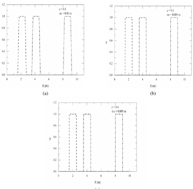
In order to verify the TVD and RCM implementations, a one-dimensional test which tracks the movement of a square pulse is used. The simulations were carried out in a uniform grid, using TVD in Fig. 2 and RCM in Fig. 3. Wave positions and shapes are verified after 1.5 s, 3.5 s and 8 s. The agreement with the analytical solution is remarkable if the stability range of the Courant number is respected.
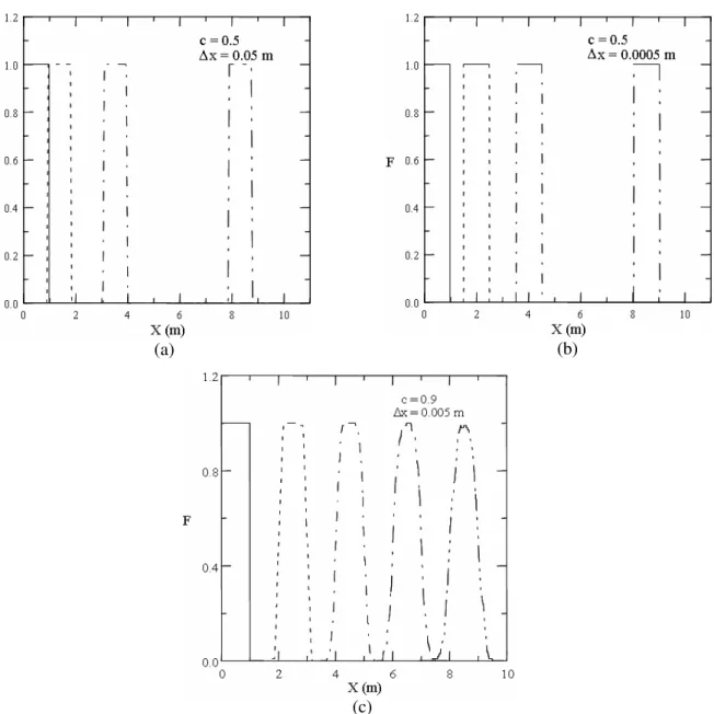
Fig. 3 shows that all RCM results perfectly resolve the contact discontinuity of the interface. However, comparing Figs. 3-a and 3-b it is clear that some inaccuracy exists in the propagated pulse position for coarse grids. This results from errors in the pulse propagation velocity due to the random character of the method. For the finer grid (Fig. 3-b), these errors basically disappear because of the large increase in the quantity of random numbers used to obtain the solution due to the Courant number limitation.
These errors in the position of the contact discontinuities are equivalent to numerical diffusion. This can be seen Fig. 3-c, which shows the mean results of one hundred simulations of the pulse tracking in the coarse grid with different seeds in the random number generator. The behavior of the shape of the propagated pulse is similar to that usually achieved in a single simulation when a diffusive scheme is used. In other words, the uncertainty in the positions of the discontinuities is numerically equivalent to the numerical diffusion of a low-order scheme.
(a) (b)
(c)
Figure 2: Square pulse propagation in a uniform grid with constant velocity u = 0.1 m/s for
(a) (b)
(c)
Figure 3: Square pulse propagation in an uniform grid with constant velocity u = 0.1 m/s using the RCM
scheme: (a) and (b) show the results for one simulation where the exact positions of the beginning of the propagated pulses are x = 1.5, 3.5 and 8.0 m; (c) shows the mean of 100 simulation results where the
exact positions of the beginning of the propagated pulses are x = 2, 4, 6 and 8.0 m.
TWO-DIMENSIONAL SIMULATION OF CAVITY FILLING
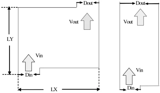
In order to compare the effectiveness of the TVD and RCM methods associated with the VOF scheme without any perturbation in the flow field, we decided to study the cavity filling using the steady-state flow solution. Two 2-D cavities are used, as shown in Figs. 4-a and 4-b. Dimensions of the mold cavity used were LY = 20 cm and LX = 30.3 cm. The dimensions of the backward facing step (BFS) cavity were 0.1m × 3.0 m.
In a cavity such as the one shown in Fig. 4-a, referred to from now on as mold cavity, a non-recirculating flow with a low Reynolds number
inlet is also parabolic, but the mean velocity is equal to 1 m/s. Due to the dimensions of this cavity ( LY 30LX= ), it is possible to apply continuity conditions for the velocities and the pressure at its outlet (Gartling, 1990). The inlet width is
in
D =0.5LX and the outlet width is LX itself. Impenetrable walls and non slip conditions are also imposed on the other walls of this cavity. Simulations use a 200 × 200 grid for the mold cavity and a 200 × 500 grid for the BFS cavity. A time step of 10-3 s was adequate for all TVD simulations and
the BFS-RCM simulations. However, the mold-RCM simulations needed a longer time step (10-1 s)
due to a loss of accuracy of the RCM for low Courant numbers, which is explained in the next section (see the remarks concerning Fig. 9).
As mentioned in Section 2, a power-law scheme is used. The grid Peclet number is defined by
Equation (23), where ? the grid length is in the appropriate direction (X or Y).
ref V
Pe Re= ∆ζϕ
Γ (23)
It is well known that power-law schemes allow numeric diffusion when the grid Peclet number exceeds 10 and the flow is oblique in relation to the grid (Patankar, 1980). In fact, in the BFS simulations, between the recirculating zones, there are Peclet numbers as high as 50 or 60. However, this phenomenon does not invalidate the conclusions of this work because our goal is to compare two surface tracking methods under the same fluid dynamic conditions. Furthermore, as observed in Section 2, velocity and pressure profiles had been successfully tested against Gartling’s benchmark.
LX LY
Din
Din
Dout Dout
Vin
Vin
Vout Vout
Figure 4: Two-dimensional cavities: (a) rectangular mold. (b) backward facing step.
SIMULATION RESULTS
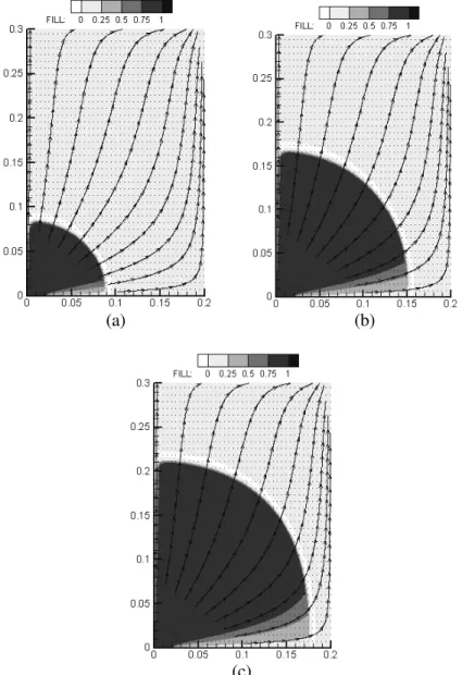
Figs. 5 and 6 compare the results achieved with the VOF-TVD scheme and the VOF-RCM scheme, respectively, for the nonrecirculating flow inside the mold cavity. The filling patterns are very similar, but a remarkable difference has to be pointed out: as filling continues the TVD scheme loses interface sharpness due to a growing diffusion effect, while the RCM scheme does not show any diffusion. It can be observed that the TVD solution shows the interface deeper inside the cavity than the RCM solution, although the same amount of fluid has entered the mold in both cases. Observing the
behavior of the solutions near the bottom wall, it becomes clear that this difference may be explained by the diffusive characteristic of the two-dimensional TVD scheme, which pushes the incoming fluid towards the top wall, allowing the other fluid to remain in the region close to the bottom wall. Due to its statistical characteristic, RCM shows an interface with small fluctuations, which tends to disappear as the filling continues.
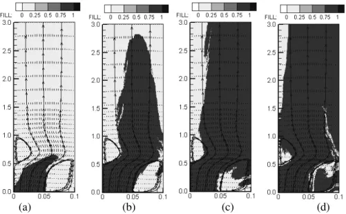
method is able to describe the droplets that are pulled away from the colored fluid by the rotating colorless fluid. The VOF-TVD scheme is unable to describe this process. Furthermore, it shows intense numerical diffusion in these regions, which can be seen in Figs. 7-b, 7-c and 7-d.
It is important to point out that Courant number restrictions remain in these two-dimensional simulations. As a matter of fact, Fig. 9-b shows that the VOF-RCM scheme is unable to track the interface when Courant numbers are less than 10-3. It
produces unrealistic results. On the other hand, the VOF-TVD scheme (Fig. 9-a) does not show the
same problem and tracks the interface perfectly. It is important to point out that all the simulations described above show an error in mass conservation of less than 5%, except for the simulations using the VOF-RCM scheme shown in Fig. 9-b.
Although the VOF-RCM scheme resolves the interface perfectly, it must be pointed out that with different seeds in the random number generator, different simulated results are obtained, even though their overall filling patterns are similar. Thus, both VOF-TVD and VOF-RCM schemes seem to be adequate to describe the overall picture of the filling pattern in the mold and the BFS cavities.
(a) (b)
(c)
Figure 5: Mold filling using the VOF-TVD scheme with LX = 0.2 m
(a) (b)
(c)
Figure 6: Mold filling using the VOF-RCM scheme with LX = 0.2 m
(∆x =10-3 m) after (a) 10 s; (b) 40 s; (c) 70 s.
(a) (b) (c) (d)
Figure 7: BFS cavity filling using the VOF-TVD scheme (∆x = 5.10-4 m) after
(a) (b) (c) (d)
Figure 8: BFS cavity filling using the VOF-RCM scheme (∆x = 5.10-4 m)
after (a) 0.5 s; (b) 3.5 s; (c) 6.5 s; (d) 9.5 s.
(a) (b)
Figure 9: Low Courant number mold filling: comparison between
VOF-TVD (a) and VOF-RCM (b) performances.
CONCLUSIONS
It was shown that the VOF-RCM scheme is able to generate diffusion-free results, sharply defining the interface, even when topological changes (droplet generation) occur due to intense recirculating flow. However, the statistical nature of RCM demands fine grids in order to simulate the interface position correctly. On the other
ACKNOWLEDGEMENTS
The authors acknowledge the financial support obtained from CNPq under grant number 520660/98-6.
NOMENCLATURE
Ci Courant number in direction I (-)
Din inlet width, M
Dout outlet width, M
F color function (-)
ˆF Riemann problem solution (-)
gi body force in i direction, m/s2
P pressure, Pa
P adimensional pressure (-)
Reref inlet Reynolds number (-)
t time, s
T stress tensor, Kg/m.s2
U velocity component in x
direction,
m/s
V velocity component in y
direction,
m/s
vmed mean inlet velocity, m/s
Y spatial coordinate, m
X spatial coordinate, m
β, γ coefficients in upwind scheme (-)
θn random number ∈ [0,1] (-)
Γ
adimensional viscosity (-)ϕ adimensional density (-)
dφi limited flux for face I (-)
ρ fluid density, Kg/m3
ρref inlet density, Kg/m3
µ fluid viscosity, Pa.s
µref inlet viscosity, Pa.s
τ
adimensional time (-)ξ transported variable (-)
∆ deviation associated with a
quantity (-)
REFERENCES
Chakravarthy, S.R. and Osher, S., A New Class of High Accuracy TVD Schemes for Hyperbolic Conservation Laws, AIAA paper 85-0363 (1985).
Colella, P., Glimm’s Method for Gas Dynamics, SIAM J. Sci. Stat. Comput., vol. 3, no. 1, pp. 76-110 (1982).
Ferziger, J.H and Pèric, M., Computational Methods for Fluid Dynamics, Springer, New York (1997). Fontes, C.E., Lage, P.L.C. and Pinto, J.C., Filling of
Rectangular Molds Using the VOF Method and a TVD Discretization, Proceedings of the XV Brazilian Congress of Mechanical Engineering (Cobem), Águas de Lindóia, São Paulo, Brazil (1999).
Gartling, D.K., A Test Problem for Outflow Boundary Conditions - Flow over a Backward Facing Step, International Journal for Numerical Methods in Fluids, vol. 11, pp. 953-967 (1990). Glimm, J., Solution in the Large for Nonlinear
Hyperbolic Systems of Equations. Comm. Pure. Appl. Math., vol. 18, pp. 697-715 (1965).
Godunov, S.K., A finite difference method for the numerical computation of discontinuous solutions of the equations of fluid dynamics, Mat. Sb., vol. 47, pp. 357-393 (1959).
Goodman, J.B. and LeVeque, R.J., On the Accuracy of Stable Schemes for 2-D Scalar Conservation Laws, Math. Comp., vol. 45, p. 15 (1985).
Osher, S. and Chakravarthy, S., Very High Order Accurate TVD Schemes, ICASE Report no. 84-44, ICASE – NASA Langley Research Center, Hampton, Virginia (1984).
Patankar, S.V., Numerical Heat Transfer and Fluid Flow, McGraw-Hill, New York (1980).
Silva, L.F.L.R. and Lage, P.L.C., Método de Escolha Aleatória em Malhas Não Uniformes: Solução da Equação da Advecção Unidimensional, 4º Congresso Brasileiro de Engenharia Química em Iniciação Científica – COBEC-IC, Maringá – PR (CD-ROM) (2001).
Sweby, P.K., High Resolution Schemes Using Flux Limiters for Hyperbolic Conservation Laws, SIAM Journal of Numerical Analysis, vol. 21, no. 5, pp. 995-1011 (1984).
Toro, E.F., Riemann Solvers and Numerical Methods for Fluid Dynamics - A Practical Introduction, 2nd Edition, Springer (1999).