A two-dimensional linear elasticity problem for anisotropic
materials, solved with a parallelization code
Mihai-Victor PRICOP*, Cornelia NI
ŢǍ
*
*Corresponding author
*INCAS – National Institute for Aerospace Research “Elie Carafoli”
Bdul Iuliu Maniu 220, Bucharest 061136, Romania
[email protected], [email protected]
Abstract: The present paper introduces a numerical approach of static linear elasticity equations for
anisotropic materials. The domain and boundary conditions are simple, to enhance an easy implementation of the finite difference scheme. SOR and gradient are used to solve the resulting linear system. The simplicity of the geometry is also useful for MPI parallelization of the code.
Key Words: elasticity, finite difference.
1. INTRODUCTION
The problem discussed in this paper does not have an immediate application. We try only to experiment the numerical methods and their algorithm, in order to obtain the numerical optimization of composite structures. The statement of the two-dimensional, anisotropic and static elasticity on a simple geometry is a good starting point for an immediate experimentation of various algorithms and parallel computing.
2. THE TWO-DIMENSIONAL ELASTICITY EQUATIONS
The equations of equilibrium, general constitutive law and deformation equations are:
0
0 xy x
y xy
x y
y x
(1)
11 12 13
21 22 23
31 32 33
x x
y y
xy x
e
e
e
e
e
e
e
e
e
y
(2)
x
u
x
,
yv
y
,
u
v
For an isotropic material, the matrix e is:
1
0
1
0
(1
)(1 2 )
1 2
0
0
2
E
e
(4)Replacing the deformations in the equations of equilibrium two partial derivative equations can be obtained, where the unknowns are the displacements.
With the following notation:
11 12 13 1 2 3
21 22 23 4 5 6
31 32 33 7 8 9
e e e e e e
e e e e e e
e e e e e e
(5)
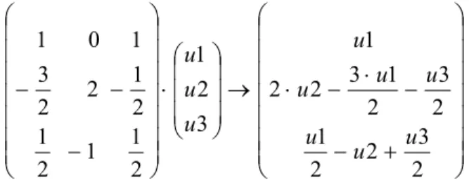
The equations in displacements are:
2 2 2 2 2 2 2 2
1 2 2 3 2 7 8 2 9 2
2 2 2 2 2 2 2 2
4 5 2 6 2 7 2 8 9 2
0
0
u
v
u
v
u
v
u
v
e
e
e
e
e
e
x
x y
x y
x
x y
y
y
x y
u
v
u
v
u
v
u
v
e
e
e
e
e
e
x y
y
y
x y
x
x y
x y
x
(6)
The domain is a rectangle, corresponding to an infinite thickness plate, with clamped edges and with imposed displacements on upper side for an easier implementation.
The grid is
1,nx0
[1,ny].The imposed Dirichlet boundary conditions are:
1. on the left side,
x
1,
y
[1,
n
y]
whereu
0;
v
0
; 2. on the right side,x
n
x0,
y
[1,
n
y]
whereu
0;
v
0
;3. on the upper side,
x
[1,
n
x0],
y
n
x0 where u0;v 0.2n xy
1x
; 4. on the lower side,x
[1,
n
x0],
y
1
whereu
0;
v
0
;The stress boundary conditions are stated as follows:
We exemplify on the left side, where imposed pressure (linear distribution load in 2D or on surface in 3D) gives:
1 2 3 1 2 3
x x y xy
u
v
u
e
e
e
e
e
e
v
x
y
y
x
(7) 4 2 1 1 1 1 0 0 1 2 3 2 2 1 2 3 2 1 3 2 2 1 3 2 1 2 1 1 2 1 2 1 2 2 3 1 0 1 u u u u u u u u u u
Fig. 1VanderMonde matrix of linear system from which results
the interpolation polynomial
Fig. 2 The inversion and multiplicationwith nodal values give the polynomial coefficients. We consider:
1
i
u
u
,u
2
u
i1,j,u
3
u
i2,j.Thus the first order derivative of the interpolation polynomial in the point x0 gives:
1, 2,
1.5
i2
i j0.5
iu
u
u
u
x
j
(8)Therefore, finite difference equation for the boundary condition is:
, 1 , 1 , 1 , 1
1 1.5 , 2 1, 0.5 2, 2 3 3 1.5 , 2 1, 0.5 2,
2 2
i j i j i j i j
i j i j i j i j i j i j x
v v u u
e u u u e e e v v v
Similarly we can apply stress boundary condition where we have a linear combination of strain, including those which are not parallel with the system axis.
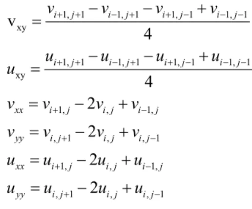
For the interior points of grid we use a centered finite difference scheme of second-order accuracy and for boundary points we use a non-centered finite difference scheme of the same order of accuracy.
Thus, considering unitary step of grid we use the formulas:
2
1, , 1,
2
2
, 1 , , 1
2
2
1, 1 1, 1 1, 1 1, 1
2
2
i j i j i j
i j i j i j
i j i j i j i j
u
u u u
x u
u u u
y u
u u u u
x y (9)
The following finite difference equation is obtained:
, 1 1, 1, 2 9 3 7 3 8 9 , 1 , 1
1 9
, 9 1, 1, 4 9 6 8 6 7 5 , 1 , 1
5 9
1 2
1 2
i j i j i j xy xy xx yy i j i j
i j i j i j xy xy yy xx i j i j
u e u u e e v e e u e v e v e u
e e
v e v v e e u e e v e u e u e v
Where:
1, 1 1, 1 1, 1 1, 1 xy
1, 1 1, 1 1, 1 1, 1
xy
1, , 1,
, 1 , , 1
1, , 1,
, 1 , , 1
v
4
4 2
2 2 2
i j i j i j i j
i j i j i j i j
xx i j i j i j yy i j i j i j xx i j i j i j yy i j i j i j
v v v v
u u u u
u
v v v v
v v v v
u u u u
u u u u
(10)
3. POST PROCESSING
The results are obtained for any boundary conditions in terms of displacement. For the post processing the stress and the strain are needed in the entire domain. The computation is very simple for the inner nodes
i
2 :
n
x0
1
j
2 :
n
y
1
.Because of the computational inefficiency, Jacobi and simple gradient methods were implemented serial only. Conjugated gradient methods will be approach in the future.
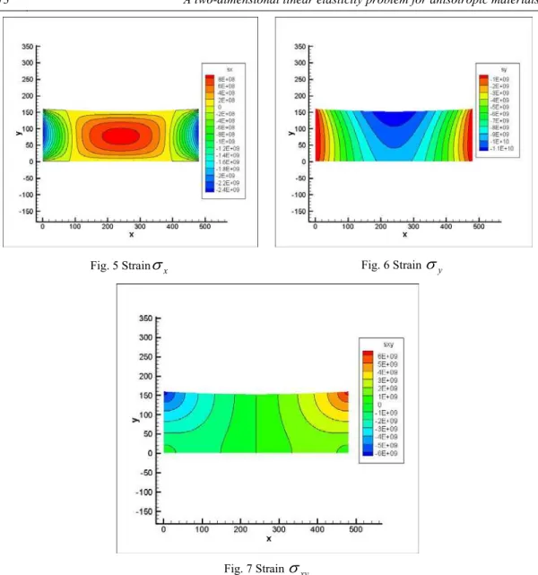
4. RESULTS
Serial SOR Gauss-Seidel
This method is an order of magnitude more efficient than Jacobi in terms of iterations number or computational time.
Fig. 5 Strain
x Fig. 6 Strain
yFig. 7 Strain
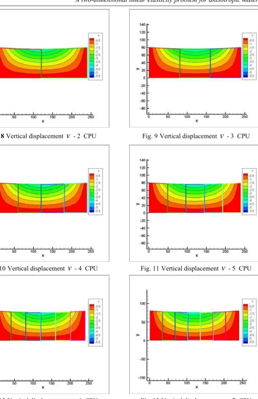
xyParallel SOR Gauss-Seidel
The parallelization for computers with distributed memory architecture, calls the one-dimensional partition.
The displacements matrices are divided in blocks horizontally aligned. Any computing node array (displacements) is one column extended in both directions, in order to store neighbors values used as boundary conditions.
0
Serial Jacobi
x y
n
n
iterations accuracy Time[s]120 x 40 5575 8
10
18.84 240 x 80 16600 71.5 10
235.28Serial SOR Gauss-Seidel
0
x y
n
n
iterations accuracy Time[s]120 x 40 475 8
10
1.77 240 x 80 1719 810
25.46 360x 120 3573 810
120.28 480x 160 5982 810
363.64Parallel SOR Gauss-Seidel 2 CPU
0
x y
n
n
iterations accuracy Time[s]120 x 40 378 8
10
0.6 240 x 80 1477 810
7.38 360x 120 3229 810
38.06Parallel SOR Gauss-Seidel 3 CPU
x0 y
n
n
iterations accuracy Time[s]120 x 40 389 8
10
0.53 240 x 80 1487 810
5.27 360x 120 3228 810
25.52Parallel SOR Gauss-Seidel 4 CPU
0
x y
n
n
iterations accuracy Time[s]120 x 40 395 8
10
0.46 240 x 80 1493 810
4.34 360x 120 3247 810
20.03Parallel SOR Gauss-Seidel 5 CPU
x0 y
n
n
iterations accuracy Time[s]120 x 40 401 8
10
0.25 240 x 80 1512 810
3.10 360x 120 3268 810
16.77Parallel SOR Gauss-Seidel 6 CPU
0
x y
n
n
iterations accuracy Time[s]120 x 40
411
810
0.36
240 x 80
1523
810
2.93
360x120 3283
810
12.99
Parallel SOR Gauss-Seidel 7 CPU
x0 y
n
n
iterations accuracy Time[s]120 x 40 419 8
10
0.34 240 x 80 1541 810
2.16 360x 120 3309 810
11.66Parallel SOR Gauss-Seidel 8 CPU
x0 y
n
n
iterations accuracy Time[s]120 x 40 426 8
10
0.36 240 x 80 1555 810
2.42 360x 120 3326 8Fig. 8Vertical displacement v - 2 CPU Fig. 9Vertical displacement v - 3 CPU
Fig. 10Vertical displacement v - 4 CPU Fig. 11Vertical displacement v - 5 CPU
Fig. 14Vertical displacement v - 8 CPU
Fig. 15Computational time for one iteration, for the 3 discretization types: p(120x40), q(240x80), r(360x120), according tothe processor number.
Fig. 16 Effective computational time for the 3 discretization types according to theprocessors number.
5. CONCLUSIONS
Future work will focus on utilization of finite difference scheme of fourth order accuracy and also parallel form of conjugate gradient algorithm.
It is also interesting to implement this code for the three dimensional elasticity problems for both isotropic and anisotropic materials.
REFERENCES
[1] A
.
Neculai,
Convergenta algoritmilor de optimizare, Editura Tehnica, 2004.[2] M. Snir, S. Otto, S. Huss-Lederman, J. Dongara, MPI: The Complete Reference, the MIT Press, Cambridge, Massachusetts, 1996.