A moving point approach to model shallow ice sheets: a study case with radially-symmetrical ice sheets

(1)

TCD

9, 4237–4270, 2015

Moving point approach to model shallow ice sheets in

radially-symmetrical cases

B. Bonan et al.

Title Page

Abstract Introduction

Conclusions References

Tables Figures

◭ ◮

Back Close

Full Screen / Esc

Printer-friendly Version

Interactive Discussion

Discussion

P

a

per

|

Discussion

P

a

per

|

Discussion

P

a

per

|

Discussion

P

a

per

|

The Cryosphere Discuss., 9, 4237–4270, 2015 www.the-cryosphere-discuss.net/9/4237/2015/ doi:10.5194/tcd-9-4237-2015

This discussion paper is/has been under review for the journal The Cryosphere (TC). Please refer to the corresponding final paper in TC if available.

A moving point approach to model

shallow ice sheets: a study case with

radially-symmetrical ice sheets

B. Bonan, M. J. Baines, N. K. Nichols, and D. Partridge

School of Mathematical and Physical Sciences, University of Reading, Reading, UK

Received: 6 July 2015 – Accepted: 10 July 2015 – Published: 7 August 2015

Correspondence to: B. Bonan (b.c.bonan@reading.ac.uk)

(2)

TCD

9, 4237–4270, 2015

B. Bonan et al.

Title Page

Tables Figures

◭ ◮

Back Close

Full Screen / Esc

Discussion

P

a

per

|

Discussion

P

a

per

|

Discussion

P

a

per

|

Discussion

P

a

per

|

Abstract

Predicting the evolution of ice sheets requires numerical models able to accurately track the migration of ice sheet continental margins or grounding lines. We introduce a physically-based moving point approach for the flow of ice sheets based on the conservation of local masses. This allows the ice sheet margins to be tracked explicitly

5

and the waiting time behaviours to be modelled effi_{ciently. A finite di}ff_{erence moving}

point scheme is derived and applied in a simplified context (continental radially-symmetrical shallow ice approximation). The scheme, which is inexpensive, is validated by comparing the results with moving-margin exact solutions and steady states. In both cases the scheme is able to track the position of the ice sheet margin with high

10

precision.

1 Introduction

Ice loss in Greenland and Antarctica accounts for a large fraction of today’s sea-level rise (Church et al., 2013). This ice loss modifies the ice flow but also translates into the retreat of continental margins (in Greenland) and grounding lines (mainly in Antarctica).

15

Predicting the evolution of both aspects is essential in order to accurately estimate their future contribution to sea-level change. However, simulating the migration of an ice sheet margin or a grounding line remains a complex task (see e.g. Vieli and Payne, 2005; Pattyn et al., 2013). This paper introduces a moving point method for the numerical simulation of ice sheets, especially the migration of their boundaries. In

20

this paper we focus on the migration of continental ice sheet margins.

At the scale of an ice sheet or a glacier, ice is modelled as a flow which follows the Stokes equations of fluid flows (Stokes, 1845), even though the flow is non-Newtonian and its rheology is highly nonlinear. Solving this problem at that scale is costly. A 3-D finite element model called Elmer/Ice has been developed for this purpose

25

numerically (see Gagliardini et al., 2013 for a detailed description of Elmer/Ice). Other

(3)

TCD

9, 4237–4270, 2015

B. Bonan et al.

Title Page

Tables Figures

◭ ◮

Back Close

Full Screen / Esc

Discussion

P

a

per

|

Discussion

P

a

per

|

Discussion

P

a

per

|

Discussion

P

a

per

|

models take advantage of the very small aspect ratio of ice sheets and use a thin layer approximation diff_{ering only in the order of the approximation. The oldest and}

numerically least expensive model used for ice flow is the Shallow Ice Approximation or SIA (Hutter, 1983). It gives an analytical formulation for horizontal velocities of ice in the sheet and for their vertically averaged counterpart. Although simple and fast,

5

the SIA captures well the nonlinearity of the system and is an excellent resource for testing numerical approaches, since moving-margin exact solutions exist in the literature (Halfar, 1981, 1983; Bueler et al., 2005).

Significant eff_{orts have been invested in ice sheet modelling. These have led}

ice sheet modellers to compare results obtained by various models for the same

10

idealistic test problems (see the EISMINT intercomparison project (Huybrechts et al., 1996; Payne et al., 2000) for ice sheet models using SIA). Most numerical ice sheet simulations use a fixed grid to calculate the solution of the ice flow equations. In fixed grid models the ice sheet margins are not precisely located as they generally fall between grid points. So in order to obtain a good approximation a high grid resolution is

15

required around the positions of the ice sheet margin during its evolution, which makes fixed grid models costly for accurately computing the evolution of the ice margin.

One approach to gain high resolution is to apply adaptative grid techniques, which allow improved resolution to be achieved in key areas. For example, Cornford et al. (2013) apply adaptative mesh refinement (AMR) in the case of marine ice sheets

20

and grounding line migration. However, even with AMR, the ice sheet margin still falls between grid points, although by adapting the grid to increase the resolution near the margin, the accuracy is kept high. Adapting the grid is, nevertheless, an expensive procedure, as areas where refinement is needed have to be regularly re-identified.

Another possibility is to transform the moving domain. The number of grid points is

25

(4)

TCD

9, 4237–4270, 2015

B. Bonan et al.

Title Page

Tables Figures

◭ ◮

Back Close

Full Screen / Esc

Discussion

P

a

per

|

Discussion

P

a

per

|

Discussion

P

a

per

|

Discussion

P

a

per

|

along a flowline. However, it is not easily translated into two dimensions and no pure transformed grid ice sheet model has been published.

We consider here intrinsically moving grid methods. As in the case of transformed grids, these methods allow explicit tracking of the ice sheet margin. There exists a number of techniques for generating the nodal movement in moving grid methods.

5

They can be classified into two subcategories, location-based methods and velocity-based methods (Cao et al., 2003). In location-velocity-based methods the positions of the nodes are redefined directly at each time step by a mapping from a reference grid (Budd et al., 2009). This is generally done by choosing a monitor function. In velocity-based methods, on the other hand, the movement of the nodes is defined in terms of

10

a time-dependent velocity, which allows the nodes to be influenced by their previous position (Baines et al., 2005, 2011). Currently, this approach has not been applied to the dynamics of ice sheets and we address the issue in this paper.

In this paper, we apply a particular velocity-based moving point approach based on conservation of local mass fractions to continental ice sheets. We derive a finite

15

diff_{erence moving point scheme in a simplified context and validate the approach}

with known exact solutions in the case of radially-symmetrical ice sheets. We show in particular that the scheme is able to track the position of the ice sheet margin accurately. The paper is organised as follows: in Sect. 2 we recall the SIA and detail the simplified context of our study, in Sect. 3 we describe our velocity-based moving point

20

approach, and in Sect. 4 we validate our approach by comparison with exact solutions before concluding in Sect. 5.

2 Ice sheet modelling

2.1 Ice sheet geometry and Shallow Ice Approximation

We consider a single solid phase ice sheet whose thickness at position (x,y) and time

25

t is denoted by h(t,x,y). We assume that the ice sheet lies on a fixed bedrock and

(5)

TCD

9, 4237–4270, 2015

B. Bonan et al.

Title Page

Tables Figures

◭ ◮

Back Close

Full Screen / Esc

Discussion

P

a

per

|

Discussion

P

a

per

|

Discussion

P

a

per

|

Discussion

P

a

per

|

denote byb(x,y) the bed elevation. The surface elevation,s(t,x,y), is then obtained as

s=_b+_h ₍₁₎

The evolution of ice sheet thickness is governed by the balance between ice gained or lost on the surface, snow precipitation and surface melting, and ice flow draining ice

5

accumulated in the interior towards the edges of the ice sheet. This is summarised in the mass balance equation

∂h

∂t =m− ∇ ·(hU) in Ω(t) (2)

where m(t,x,y) is the surface mass balance (positive for accumulation, negative for ablation), U₍_t_,_x_,_y_{) is the vector containing the vertically averaged horizontal}

10

components of the velocity of the ice, and Ω₍_t_{) is the area where the ice sheet is}

located.

Formally derived by Hutter (1983), the Shallow Ice Approximation (SIA) is one of the most common approximations for large-scale ice sheet dynamics. Combined with Glen’s flow law (Glen, 1955), the SIA provides (in the isothermal case) an analytical

15

formulation forU _{as follows:}

U=₋ 2

n+₁A(ρig)

n_hn+₁

|∇s|n−1∇s (3)

Parameters involved in this formulation are summarised in Table 1. Regarding the exponentn >1, its fixed value is classically set to 3 (see Cuff_{ey and Paterson, 2010,}

for more details).

20

2.2 Radially-symmetrical ice sheets

(6)

TCD

9, 4237–4270, 2015

B. Bonan et al.

Title Page

Tables Figures

◭ ◮

Back Close

Full Screen / Esc

Discussion

P

a

per

|

Discussion

P

a

per

|

Discussion

P

a

per

|

Discussion

P

a

per

|

study to limited area ice sheets with radial symmetry, in other words,Ω₍_t₎ =_[0,_r

l(t)]× [0, 2π]. The ice sheet is centred on (0, 0) andrl(t) denotes the position of the ice sheet margin (edge of the ice sheet) at timet (see Fig. 1). The radial symmetry implies that the geometry of the sheet depends only on r, so h(t,x,y)=_h₍_t_,_r_), _s₍_t_,_x_,_y₎=_s₍_t_,_r₎

andb(x,y)=_b₍_r_{). The vector}U _{can then be written in the radial coordinate system as}

5

U=_Ur_ˆ_, _U =₋ 2

n+₂A(ρig)

n_hn+₁

∂s ∂r

n−1_∂s

∂r (4)

where ˆr _{is the unit radial vector, and the mass balance Eq. (2) simplifies to}

∂h ∂t =m−

1 r

∂(r h U)

∂r (5)

A symmetry condition is added at the ice divide (r =_0):

U=₀ _and ∂s

∂r =0, (6)

10

and the ice sheet marginr_l(t) is characterised by the Dirichlet boundary condition:

h(t,r_l(t))=₀ ₍₇₎

We also assume that the flux of ice through the ice sheet margin is zero (no calving). The aim of this paper is to propose a moving point numerical method able to accurately simulate the evolution of the ice sheet margin. Under some hypotheses

15

regarding the regularity of the ice thickness near the margin (see Calvo et al., 2002), we can diff_{erentiate Eq. (7) with respect to time. If}_∂h/∂r _{does not tend to zero near}

the margin, we obtain the following equation

drl

dt =U(t,rl(t))−m(t,rl(t)) _∂h

∂r −1

(8)

This equation (Eq. 8) will be used in the moving point approach described in the next

20

section.

(7)

TCD

9, 4237–4270, 2015

B. Bonan et al.

Title Page

Tables Figures

◭ ◮

Back Close

Full Screen / Esc

Discussion

P

a

per

|

Discussion

P

a

per

|

Discussion

P

a

per

|

Discussion

P

a

per

|

3 A moving point approach

In the following paragraphs we describe the moving point method that we use to simulate the dynamics of ice sheets in the context of Sect. 2.2. This method is essentially a velocity-based (or Lagrangian) method relying on the construction of velocities for grid points at each instant of time. This allows the grid to move with

5

the flow of ice. Moving points cover the domain only where the ice sheet exists, so that no grid point is wasted. Adjacent points move to preserve local mass fractions and the movement is thus based on the physics (Blake, 2001; Baines et al., 2005, 2011; Scherer and Baines, 2012; Lee et al., 2015). This conservation method has been applied in various contexts and is perfectly suitable for multi-dimensional problems

10

(diff_{erent examples are summarised in Baines et al. (2011) and references therein;}

see also Partridge (2013) for the special case of ice sheet dynamics). The key points of the method are given in the next paragraphs and the numerical validation of the method is carried out in Sect. 4.

3.1 Conservation of mass fraction

15

Moving point velocities are derived from the conservation of mass fractions (CMF). To apply this principle we first define the total mass of the ice sheetθ(t) as

θ(t)=₂_π

rl(t) Z

0

r h(t,r) dr (9)

In factθ(t) is the total volume of the ice sheet but, since the density of ice is assumed constant everywhere, θ(t) is proportional to the total mass of the ice sheet and the

20

constant of proportionality cancels out.

(8)

TCD

9, 4237–4270, 2015

B. Bonan et al.

Title Page

Tables Figures

◭ ◮

Back Close

Full Screen / Esc

Discussion

P

a

per

|

Discussion

P

a

per

|

Discussion

P

a

per

|

Discussion

P

a

per

|

m(t,r), and hence the rate of change of the total mass, ˙θ, is given by

˙

θ(t)=₂_π

rl(t) Z

0

r m(t,r) dr (10)

We now introduce the principle of the conservation of mass fractions. Let ˆr(t) be a moving point and defineµ( ˆr) to be therelativemass in the moving subinterval (0, ˆr(t)) as

5

µ( ˆr)= 2π

θ(t)

ˆ

r(t)

Z

0

r h(t,r) dr (11)

The rate of change of ˆr(t) is determined by keeping µ( ˆr) independent of time for all moving subdomains of [0,r_l(t)]. Note that µ( ˆr)∈[0, 1] is a cumulative function with µ(0)=_{0 and}_µ₍_r

l)=1.

3.2 Trajectories of moving points

10

We obtain the velocity of a moving point by diff_{erentiating Eq. (11) with respect to time,}

giving

d dt

  2π

ˆ

r(t)

Z

0

r h(t,r) dr   

=_µ_{( ˆ}_r_{) ˙}_θ₍_t₎ ₍₁₂₎

Carrying out the time diff_{erentiation using Leibniz’s integral rule and substituting for}

∂h/∂tfrom the mass balance Eq. (5) gives

15

d dt

  

ˆ

r(t)

Z

0

r h(t,r) dr   

=

ˆ

r(t)

Z

0

r m(t,r) dr+_r_ˆ₍_t₎_h₍_t_{, ˆ}_r₍_t₎₎

_d_r_ˆ

d t−U(t, ˆr(t))

(13)

(9)

TCD

9, 4237–4270, 2015

B. Bonan et al.

Title Page

Tables Figures

◭ ◮

Back Close

Full Screen / Esc

Discussion

P

a

per

|

Discussion

P

a

per

|

Discussion

P

a

per

|

Discussion

P

a

per

|

with boundary conditions (Eq. 6) at r =_{0. From Eqs. (12), (13) and (10), we can}

determine the velocity of every interior point as

d ˆr

dt =U(t, ˆr(t))+

1 ˆ

r(t)h(t, ˆr(t))   µ( ˆr)

rl(t) Z

0

r m(t,r) dr−

ˆ

r(t)

Z

0

r m(t,r) dr  

 (14)

The point at r =_{0 is located at the ice divide, which does not move during the}

simulation. The point atrl(t) is dedicated to the ice sheet margin, which moves with the

5

velocity obtained in Eq. (8). We verify in Appendix A that the interior velocity calculated by Eq. (14) coincides with the boundary velocities calculated directly from the boundary conditions (see Eq. 8).

3.3 Determination of the ice thickness profile

Once the velocities d ˆr/dtof the moving points ˆr(t) have been found from Eq. (14), the

10

points are moved in a Lagrangian manner. In addition, the total massθ(t) is updated from Eq. (10). The ice thickness profile is then deduced from Eq. (11) as follows. Diff_{erentiating Eq. (11) with respect to ˆ}_r2_{, we obtain}

h(t, ˆr(t))=θ(t)

π

dµ( ˆr)

d( ˆr2₎ (15)

which allows the ice thickness profile at timet to be constructed since dµ( ˆr)/d( ˆr2) is

15

constant in time and therefore known from the initial data. Note that the positivity of the ice thickness is preserved sinceµis by definition a strictly increasing function (see Eq. 11).

3.4 Asymptotic behaviour at the ice sheet margin

As pointed out by Fowler (1992) and Calvo et al. (2002), with SIA singularities can

20

(10)

TCD

9, 4237–4270, 2015

B. Bonan et al.

Title Page

Tables Figures

◭ ◮

Back Close

Full Screen / Esc

Discussion

P

a

per

|

Discussion

P

a

per

|

Discussion

P

a

per

|

Discussion

P

a

per

|

vanishing of h at the margin and the steepening of the slope ∂h/∂r. Nevertheless the ice velocityU defined by Eq. (4) can remain finite even if the slope is infinite. We give more details on this subject in this subsection. We also detail the influence of the singularity on the movement of the ice sheet margin.

At a fixed time and for pointsr suffi_{ciently close to}_r

l, we can write the ice thickness

5

profileh(r) as the first term in a Frobenius expansion

h(r)=₍_r

l−r)γgl (16)

to leading order, wheregl =O(1). Ifγ=1, thenh(r) is locally linear with slopegl, but if γ <1 the slope∂h/∂ris unbounded. Hence in the asymptotic region near the margin, in the case where the bedrock topographyb(r) is constant, from Eq. (4)

10

U= 2

n+₂A(ρig)

n_γn₍_r

l−r)(2n

+₁₎γ−n_g l2n

+₁

(17)

which vanishes asr tends torl ifγ > n/(2n+1) and remains finite ifγ=n/(2n+1). Supppose that in the evolution of the solution over time,γ(t)> n/(2n+_{1) initially so}

that r_l(t) is constant and the boundary is stationary (waiting). If ˆr(t) follows a CMF trajectory then, in the absence of accumulation/ablation, the velocity of the moving

15

coordinate ˆr(t) is given by

U= 2

n+₂A(ρig)

n_γ₍_t₎n₍_r

l(t)−rˆ(t))(2n

+₁₎_γ₍_t₎₋_n

g_l(t)2n+1 (18)

Asymptotically, except at the boundary itself, this velocity is finite and positive, since U >0 and its spatial derivative ∂U/∂r <0 suffi_{ciently close to the boundary, showing}

that the distancerl(t)−rˆ(t) decreases with time.

20

In the absence of accumulation/ablation, therefore, conservation of mass fractions implies that (r_l(t)−rˆ(t))U(t, ˆr(t))g_l(t) is constant in time. Thus, from (16), for points ˆr(t) suffi_{ciently close to the boundary (}_r_l₍_t₎₋_r_ˆ₍_t₎₎γ(t)+1_g_l₍_t_{) is constant in time. Hence, since}

(11)

TCD

9, 4237–4270, 2015

B. Bonan et al.

Title Page

Tables Figures

◭ ◮

Back Close

Full Screen / Esc

Discussion

P

a

per

|

Discussion

P

a

per

|

Discussion

P

a

per

|

Discussion

P

a

per

|

(rl(t)−rˆ(t)) is decreasing,γ(t) is also decreasing. Whenγ(t) reaches n/(2n+1) the boundary moves.

It is a technical exercise to show that this property extends to cases with accumulation/ablation and with a general bedrock with a finite slope ∂b/∂r at the margin (see Partridge, 2013). The key point to notice is that the asymptotic behaviour

5

depends on an infinite slope ofhat the margin whereasb(r) always has a finite slope.

3.5 Numerics

We now implement a numerical scheme using a finite diff_{erence method. The complete}

algorithm is detailed in Appendix B. In addition, we explain in Appendix B6 why our implementation respects the asymptotic behaviour of the ice sheet at its margin.

10

4 Numerical results

This section is dedicated to the validation of the numerical scheme derived from the moving point method detailed in Sect. 3 and to the study of its behaviour. Every numerical experiment is performed with the parameter values given in Table 1.

4.1 Steady states with flat bedrock

15

We start by studying the behaviour of the numerical scheme using a surface mass balancem(r) constant in time in order to define a steady state. When the steady state is reached, from Eq. (5), the following relationship is valid:

r m= ∂

∂r(r h

∞_U∞

r ) (19)

with h∞(r) the thickness of the steady ice sheet and U∞(r) the ice velocity. By

20

(12)

TCD

9, 4237–4270, 2015

B. Bonan et al.

Title Page Abstract Introduction Conclusions References Tables Figures ◭ ◮ ◭ ◮ Back Close

Full Screen / Esc

Printer-friendly Version Interactive Discussion Discussion P a per | Discussion P a per | Discussion P a per | Discussion P a per |

the position of the marginr_l∞can be obtained from

r_l∞ Z

0

rm(r) dr =

r_l∞ Z

0

∂ ∂r(r h

∞_U∞

r ) dr=

r h∞U_r∞∞

0 =0 (20)

If the bedrock is flat, the profile of the steady ice sheet can be obtained from Eqs. (19) and (4) as

h(r)∞=

2n+₁

n ρ_ig n

n+₂

2A 2(n1+1)

   

r_l∞ Z r    1 r′ r′ Z 0

m(s)sds    1 n

dr′    

n 2(n+1)

(21)

5

Therefore, if the chosen surface mass balance is simple enough, we have an analytical formula forr_l∞ from Eq. (20) and the profile of the steady state can be approximated with high accuracy by numerical integration from Eq. (21) using a composite trapezoidal rule for example. This approach was already in use in the EISMINT intercomparison project (Huybrechts et al., 1996) with the following constant-in-time surface mass

10

balance

m(r)=_min_{0.5 m a}−1_{, 10}−2_{m a}−1_km−1_·_{(450 km}₋_r₎ ₍₂₂₎

Finding r_l from Eq. (20) requires the solution of a cubic equation. A numerical approximation isrl ≈579.81 km.

As a first test, we consider initialising our numerical model with the following profile:

15

h(t₀,r)=_h

0 1−

_r r_l(t₀)

2!p

(23)

(13)

TCD

9, 4237–4270, 2015

B. Bonan et al.

Title Page

Tables Figures

◭ ◮

Back Close

Full Screen / Esc

Discussion

P

a

per

|

Discussion

P

a

per

|

Discussion

P

a

per

|

Discussion

P

a

per

|

and study the convergence towards the steady state in three diff_{erent cases. In each}

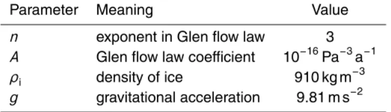
experiment, the initial grid has 21 points and the model is run for 10 000 a with a constant time step∆_t=_{0.1 a. We now detail the initial state for each experiment:}

a. Uniformly distributed initial grid withr_l(0)=_{450 km,}_h

0=1000 m andp=3/7.

b. Initial grid withrl(0)=500 km with higher resolution near the margin,h0=1000 m

5

andp=_1.

c. Uniformly distributed initial grid withr_l(0)=_{600 km,}_h

0=4000 m andp=1/4.

The evolution of the geometry and the overall motion of the grid points are shown for each experiment in Fig. 2. The three experiments show the convergence of every initial state towards the same steady state. These experiments also show the ability of the

10

CMF method to capture the trajectory of the moving ice sheet margin (in advance and retreat).

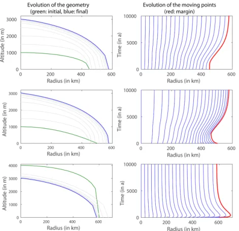
We now perform the moving-margin EISMINT experiment (Huybrechts et al., 1996) in order to validate our numerical model in this case. At the initial timet=_{0 we prescribe}

a uniformly distributed grid withrl(0)=450 km and an initial ice thicknessh(0,r) taken

15

as ∆_t_·_m₍_r_{) for the constant time step} ∆_t=_{0.1 a. Then we run the model as in the}

EISMINT experiment for 25 000 a to reach the steady state. As we also want to compare our scheme with numerical models used in EISMINT, we first perform a model run with 28 nodes. With the same number of grid points as used in the fixed grid models included in EISMINT we are able to obtain a very good estimation for the position of

20

the margin at steady state (commiting an absolute error of only 138.5 m for an exact positionr_l∞≈579.81 km) without losing accuracy on the ice thickness (see Fig. 3). The estimation of the ice thickness at the ice divide is 3005.8 m compared to 2982.3±26.4 m obtained by 2-D fixed grid models (we exclude 3-D models from our comparison as we only use radial symmetry, see Huybrechts et al., 1996) and compared to 2987±0.01 m

25

(14)

TCD

9, 4237–4270, 2015

B. Bonan et al.

Title Page

Tables Figures

◭ ◮

Back Close

Full Screen / Esc

Discussion

P

a

per

|

Discussion

P

a

per

|

Discussion

P

a

per

|

Discussion

P

a

per

|

We also study the convergence of our method towards the reference solution in this case when the number of grid points is increased. We observe that the error for the margin position decreases at an almost quadratic rate O(n1.95_r ) and the error in the ice thickness at the ice divide at a linear rateO(n1.16_r ) (results obtained by performing experiments with an initial uniformly spaced grid with nr=20, 28, 40, 60 and 80 grid

5

points).

4.2 Steady states with non-flat bedrock

The steady state approach of the previous section is still valid for an ice sheet lying on a non-flat bedrock. However, the experiments in such cases are quite limited as we only have the position of the steady margin from Eq. (20). Nevertheless we carry out

10

a few experiments in this context in order to demonstrate that the CMF moving point approach is perfectly suitable for non-flat bedrock.

We consider the following fixed bedrock elevation:

b(r)=_{2000 m}₋_{2000 m}_· r

300 km 2

+_{1000 m}_· r

300 km 4

−150 m· r

300 km

6 (24)

As in the previous section, experiments are performed with the EISMINT surface mass

15

balance (Eq. 22). At an initial timet=_{0 we prescribe a uniformly distributed grid with}

a margin located atrl(0)=450 km and an initial ice thicknessh(0,r)= ∆t·m(r) for the constant time step∆_t=_{0.1 a. The resulting evolution of the geometry and the overall}

motion of the grid points are shown for a grid of 20 points in Fig. 4. We also study the convergence of our method towards the steady state when the number of grid points

20

is increased. Again we observe that the error for the margin position decreases at a nearly quadratic rateO(n1.83_r ) (results obtained by performing experiments with an initial uniformly spaced grid andnr grid points,nr=20, 30, 40, 60 and 80).

(15)

TCD

9, 4237–4270, 2015

B. Bonan et al.

Title Page

Tables Figures

◭ ◮

Back Close

Full Screen / Esc

Discussion

P

a

per

|

Discussion

P

a

per

|

Discussion

P

a

per

|

Discussion

P

a

per

|

4.3 Validation with time-dependent solutions

In the previous paragraphs, steady states were used to validate our numerical CMF moving point numerical method. However these experiments did not validate the transient behaviour of the ice sheet margin. To do so, we use exact time-dependent solutions.

5

Few exact solutions for isothermal shallow ice sheets have been derived in the literature. Most are based on the similarity solutions established by Halfar (1981, 1983) for a zero surface mass balance. Bueler et al. (2005) extended this work to non-zero surface mass balance and established a new family of similarity solutions by adopting the following parameterised form for the surface mass balance,

10

m(ε)(t,r)=ε

th

(ε)₍_t_,_r₎ ₍₂₅₎

withεa real parameter in the interval ₂−_n₊1₁,+_∞_{. Assuming that}_{t >}_{0 this leads to the}

following family of similarity solutions

h(ε)(t,r)= 1

tα(ε) h

2n+1 n

0,1 −Λ(ε)

r tβ(ε)

n+_n1! n 2n+1

for r∈h0,tβ(ε)Θ₍_ε₎i ₍₂₆₎

with

15

α(ε)=2−(n+1)ε

5n+₃ , β(ε)=

1+₍₂_n+₁₎_ε

5n+₃ (27)

and

Λ₍_ε₎=2n+1

n+₁

₍_n₊₂₎_β₍_ε₎ 2A(ρ_ig)n

1_n

, Θ₍_ε₎=_h

2n+1 n+1

0,1 Λ(ε)

−_n+n1 (28)

The total mass of such ice sheets, as defined in Eq. (9), is

θ(ε)(t)=_β₍_ε₎−n2+1tεW

1 (29)

(16)

TCD

9, 4237–4270, 2015

B. Bonan et al.

Title Page

Tables Figures

◭ ◮

Back Close

Full Screen / Esc

Discussion

P

a

per

|

Discussion

P

a

per

|

Discussion

P

a

per

|

Discussion

P

a

per

|

whereW1is a constant independent ofε

W1=2π

Θ(1)

Z

0

s

h 2n+1

n

0,1 −Λ(1)s

n+1 n

_2nn+1

ds (30)

We study in this section the accuracy of transient model runs in comparison with the time-dependent exact solutions. The initialisation of every experiment is done by using the exact time-dependent solution (Eq. 26) and, at each time step, the surface

5

mass balance is evaluated at each moving node by using the relationshipm=ε

thfrom Eq. (25). Whenεis non-zero, somefeedbackbetween the surface mass balance and the ice thickness is expected (Leysinger Vieli and Gudmundsson, 2004). Each model run in this section uses a fixed time step of∆_t=_{0.01 a.}

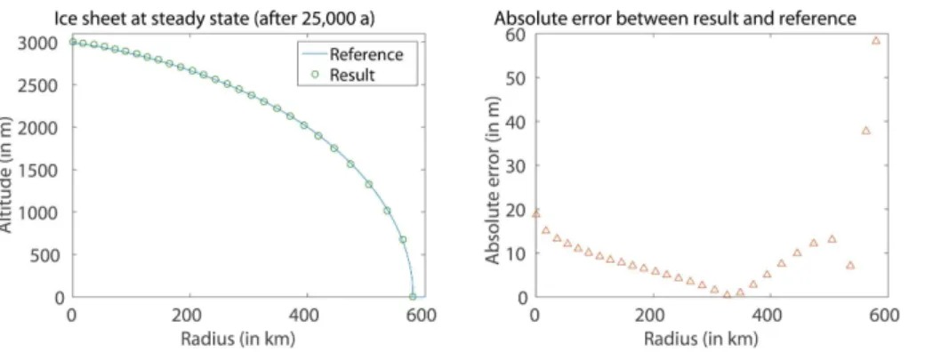
The first experiment is conducted with the constant mass similarity solution (ε=₀₎

10

betweent=_{100 a and} _t=_{20 000 a for the reference period (Fig. 5). We first analyse}

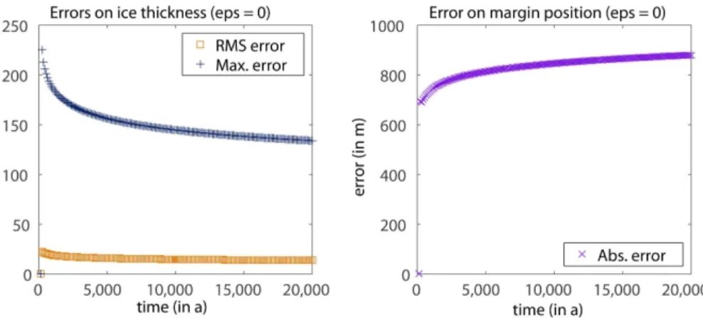
the results obtained with a grid made up of 100 nodes, uniformly distributed at the initial time. In terms of thickness, errors mostly occur near the ice sheet margin (Fig. 6) as is the case with fixed grid methods (see Bueler et al., 2005). However, the position of the ice sheet margin is well estimated, the estimated error being kept under one kilometer

15

(Fig. 7).

We then study the convergence of our scheme at a final timet=_{20 000 a when the}

number of grid points is increased. We perform the same analysis for ε=₋₁_/_{8, 1}_/₄

and 3/4. Rates of convergence for diff_{erent errors are summarised in Table 2.}

5 Conclusions

20

In this paper, we introduced a moving point approach for ice sheet modelling using the SIA (including non-flat bedrock) based on the conservation of local mass. From this principle we derived an effi_{cient finite-di}ff_{erence moving point scheme allowing}

(17)

TCD

9, 4237–4270, 2015

B. Bonan et al.

Title Page

Tables Figures

◭ ◮

Back Close

Full Screen / Esc

Discussion

P

a

per

|

Discussion

P

a

per

|

Discussion

P

a

per

|

Discussion

P

a

per

|

with steady states from the EISMINT benchmark (Huybrechts et al., 1996) and time-dependent solutions from Bueler et al. (2005). Accurate results have been obtained with a small number of grid points in both cases. Hence the comparison shows that the approach has considerable potential for future investigations.

Whilst this paper uses a vertically averaged horizontal ice velocity given by the

5

shallow ice approximation, the moving mesh scheme is independent of the form of the ice velocity used here and could be used as a solver for mass balance alongside more complex vertically-integrated approximations (see e.g. Schoof and Hindmarsh, 2010).

As mentioned earlier, the conservation approach is suitable not only for 1-D-cases

10

(flowline or radial) but also for 2-D-scenarios. A first application has been demonstrated in Partridge (2013) and will be the subject of a new paper. The conservation approach can also be applied to marine ice sheets. In these cases, diff_{erent kinds of boundaries}

have to be considered: e.g. grounding line, shelf front, and continental margin. However, the problem of initialisating such a model for use in real applications remains

15

open. The incorporation of various data assimilation procedures is currently being investigated in this context.

Appendix A: Consistency of the moving point approach at boundaries

We now verify that d ˆr/dt tends to the velocity obtained from Eq. (8) at the ice margin when ˆr(t) tends torl(t). Assuming the continuity of∂h/∂r and min the vicinity of the

20

ice sheet margin, by L’Hôpital’s rule

lim_r_ˆ₍_t₎_→_r l(t)

d ˆr

dt =U(t,rl)+limrˆ(t)→rl(t)  

˙

θ

θrhˆ (t, ˆr)−rmˆ (t, ˆr) h(t, ˆr)+_r_ˆ∂h

∂r(t, ˆr) 

(18)

TCD

9, 4237–4270, 2015

B. Bonan et al.

Title Page

Tables Figures

◭ ◮

Back Close

Full Screen / Esc

Discussion

P

a

per

|

Discussion

P

a

per

|

Discussion

P

a

per

|

Discussion

P

a

per

|

This gives

lim_r_ˆ₍_t₎_→_r_l₍_t₎d ˆr

dt =U(t,rl)−m(t,rl)

∂h ∂r(t,rl)

−1

(A2)

The limit is consistent with the velocity of the moving margin obtained in Eq. (8). The same approach can be used to show that d ˆr/dt tends to 0 when ˆr(t) tends to the ice divider=_0.

5

Appendix B: A finite difference algorithm

The moving point method is discretised on a radial line using finite diff_{erences on the}

grid{rˆ_i},i=_1,_{. . .}_,_n

r where

0=_r_ˆ

1(t)<rˆ2(t)< . . . <rˆnr−1(t)<rˆnr(t)=rl(t), (B1) The approximation ofh(t,r) at ˆri(tk)=rˆikis writtenh

k

i and that of the ice velocityU(t,r)

10

as U_ik. The velocity of the points is represented by v_ik. The symbol θk designates the numerical approximation of the total mass and the constant mass fractions are represented byµi for everyµ( ˆrik).

Before giving the formula for every quantity calculated, we give the structure of the finite diff_{erence algorithm in Algorithm 1.}

15

(19)

TCD

9, 4237–4270, 2015

B. Bonan et al.

Full Screen / Esc

Algorithm 1Finite difference moving point algorithm

Require: ˆ r0 i and h0

i ,i= 1, . . . , nrwithrˆ0₁= 0andh0nr = 0_.

1: Compute total massθ0_{with eq. (B2)}

2: Compute mass fractionsµi,i= 1, . . . , nr, with eq. (B3) 3: whilet < tenddo

4: Compute ice velocitiesUk

i with eq. (B4) and eq. (B5) 5: Compute point velocitiesvk

i with eq. (B6) and eq. (B7) 6: Update total massθk+1_{with eq. (B8)}

7: Update moving point positions_rˆ_ik+1_{with eq. (B9)}

8: Update ice thicknesshki+1with eq. (B10) and (B11) 9: k←k+ 1

10: t←t+ ∆t

11: end while

B1 Initialisation

At the initial time the user needs to provide the initial location of each grid point

{rˆ_i0} and the initial ice thickness {h0_i} there. By definition, we assume that ˆr₁0=₀

and h0_n_r=_{0. We estimate the total mass of the ice sheet at the initial time by using}

5

a composite trapezoidal rule approximating Eq. (9). This gives:

θ0=π

2 nr−1

X j=₁

h0_j +_h0

j+₁

ˆ r_j0+₁

2

−rˆ_j02

(B2)

We derive the numerical approximation for the mass fractionsµiby discretising Eq. (11) following the same principle:

µ₁=_0, _µ

i = π 2θ0

i−1

X j=₁

h0_j +_h0

j+1

ˆ

r_j0₊₁2−rˆ_j02

(B3)

(20)

TCD

9, 4237–4270, 2015

B. Bonan et al.

Full Screen / Esc

B2 Ice velocities

We confine the algorithm ton=_{3 for the exponent in the Glen flow law. Then Eq. (4)}

giving the ice velocity can be expanded by using the binomial theorem:

|U(t,r)|= 2

5A(ρig)

3 h4 _∂b ∂r 3 +3 5 ∂(h5)

∂r _∂b ∂r 2 + 1 3

∂(h3) ∂r !2 ∂b ∂r + 27 343

∂(h7/3) ∂r !3 (B4)

We choose to rewrite the radial form of Eq. (4) in this way in order to ensure that the

5

ice velocity at the ice sheet margin computed with a finite diff_{erence scheme can be}

non-zero as noted in Sect. 3.4. The bedrock elevationb and its derivative are known for every location of the domain. The sign ofU_ik (U₁k=_{0) is obtained by calculating the}

sign ofs_ik−s_ik₋₁ (approximating the sign of the surface slope by an upwind scheme). We also approximate the derivatives ofhpfor anyp >0 by an upwind scheme:

10

∂(hp) ∂r

r=r_ik

=

hk_ip−hk_i₋₁p

r_ik−r_ik₋₁ (B5)

B3 Approximate nodal velocities

The velocity of interior nodes is obtained by discretising Eq. (14) as

v₁k=_0, _vk

i =U k i +

1

2 ˆr_ikhk_i     µ_i ˆ

r_nrk Z

0

m(tk,r) dr2−

ˆ

r_ik Z

0

(21)

TCD

9, 4237–4270, 2015

B. Bonan et al.

Title Page

Tables Figures

◭ ◮

Back Close

Full Screen / Esc

Discussion

P

a

per

|

Discussion

P

a

per

|

Discussion

P

a

per

|

Discussion

P

a

per

|

where the integrals in Eq. (B6) are approximated by a composite trapezoidal rule. For the velocity of the ice sheet margin, Eq. (8) is discretised by using an order-1 upwind scheme, namely,

vnk_r =Unk_r−m

tk,rnk_r rˆ

k

n_r−rˆnkr−1 hk_n_r−hk_n

r−1

(B7)

B4 Time stepping

5

The total massθk+1is updated by using an explicit Euler scheme

θk+1=_θk+ ∆_t_θ˙k=_θk+ ∆_{t π}

ˆ

r_nrk Z

0

m(t,r)dr2 (B8)

Again the integral is approximated by a composite trapezoididal rule.

As in the case of the total mass, the position of the nodes is updated by using an explicit Euler scheme

10

ˆ

r_ik+1=_r_ˆk

i + ∆t v k

i (B9)

with∆_t_{small enough to preserve the order in Eq. (B1).}

B5 Approximate ice thickness

The ice thickness for interior nodes hk_i+1 is recovered algebraically at the new time using an order-2 midpoint approximation of Eq. (15), namely,

15

hk_i+1=θ

k+1

π

µi+₁−µi−1

ˆ

r_ik₊+₁12−rˆ_ik₋+₁12

(22)

TCD

9, 4237–4270, 2015

B. Bonan et al.

Full Screen / Esc

The ice thickness at the ice divide hk₁+1 is obtained by using the order-1 upwind scheme.

hk+1 1 =

θk+1 π

µ₂−µ₁

ˆ

r₂k+12−rˆ₁k+12

(B11)

B6 Behaviour of the approximate ice velocity at the ice margin

As in Sect. 3.4, assuming the topography of the bedrock is flat at the vicinity of the

5

margin, the asymptotic form of the radial ice velocity is

U= 2

n+₂A(ρig)

n_γn₍_r

l−r)(2n

+₁₎γ−n_g l2n

+₁

(B12)

Hence the leading term in the numerical approximation (Eq. B4) to the ice velocity at the approximationhl to the ice margin is

−2

5sgn

s_n_r−s_n_r₋₁A(ρ_ig)3 3 7 3

h7_n/_r3−h7_n/3 r−1 ˆ

rn_r−rˆn_r−1

3

=₋2

5sgn

s_n_r−s_n_r₋₁A(ρ_ig)3 3 7 3

h7_n/3 r−1 ˆ

rn_r−rˆn_r−1

3 (B13) 10

sinceh_n_r=_{0. But from Eq. (B12) the asymptotic analytic ice velocity (when}_n=_{3) is}

2

5A(ρig)

3

3 7

3

(rn_r−r)7γ−3gI7= 2

5A(ρig)

3 27

343

h(r)7/3 r_n_r−r

!3

(B14)

(23)

TCD

9, 4237–4270, 2015

B. Bonan et al.

Title Page

Tables Figures

◭ ◮

Back Close

Full Screen / Esc

Discussion

P

a

per

|

Discussion

P

a

per

|

Discussion

P

a

per

|

Discussion

P

a

per

|

by Eq. (16). Hence the numerical approximation to the ice velocity has the same asymptotic behaviour as the asymptotic analytic ice velocity withn=_{3. The result also}

holds for generaln.

Acknowledgements. This research was funded in part by the Natural Environmental Research Council National Centre for Earth Observation (NCEO) and the European Space Agency

5

(ESA).

References

Baines, M. J., Hubbard, M. E., and Jimack, P. K.: A moving mesh finite element algorithm for the adaptive solution of time-dependent partial diff_{erential equations with moving boundaries,}

Appl. Numer. Math., 54, 450–469, doi:10.1016/j.apnum.2004.09.013, 2005. 4240, 4243

10

Baines, M. J., Hubbard, M. E., and Jimack, P. K.: Velocity-based moving mesh methods for nonlinear partial diff_{erential equations, Commun. Comput. Phys., 10, 509–576,}

doi:10.4208/cicp.201010.040511a, 2011. 4240, 4243

Blake, K. W.: Moving Mesh Methods for Non-Linear Parabolic Partial Diff_{erential Equations,}

PhD thesis, available at: http://www.reading.ac.uk/web/FILES/maths/Kw_blake.pdf (last

15

access: 4 August 2015), University of Reading, Reading, Berks, UK, 2001. 4243

Budd, C. J., Huang, W., and Russell, R. D.: Adaptivity with moving grids, Acta Numerica, 18, 111–241, doi:10.1017/S0962492906400015, 2009. 4240

Bueler, E., Lingle, C. S., Kallen-Brown, J. A., Covey, D. N., and Bowman, L. N.: Exact solutions and verification of numerical models for isothermal ice sheets, J. Glaciol., 51, 291–306,

20

doi:10.3189/172756505781829449, 2005. 4239, 4251, 4252, 4253

Calvo, N., Díaz, J. I., Durany, J., Schiavi, E., and Vázquez, C.: On a doubly nonlinear parabolic obstacle problem modelling ice sheet dynamics, SIAM J. Appl. Math., 63, 683– 707, doi:10.1137/S0036139901385345, 2002. 4242, 4245

Cao, W., Huang, W., and Russell, R. D.: Approaches for generating moving adaptive

25

meshes: location versus velocity, Appl. Numer. Math., 47, 121–138, doi:10.1016/S0168-9274(03)00061-8, 2003. 4240

(24)

TCD

9, 4237–4270, 2015

B. Bonan et al.

Title Page

Tables Figures

◭ ◮

Back Close

Full Screen / Esc

Discussion

P

a

per

|

Discussion

P

a

per

|

Discussion

P

a

per

|

Discussion

P

a

per

|

Stammer, D., and Unnikrishnan, A. S.: Sea level change, in: Climate Change 2013: The Physical Science Basis. Contribution of Working Group I to the Fifth Assessment Report of the Intergovernmental Panel on Climate Change, edited by: Stocker, T. F., Qin, D., Plattner, G.-K., Tignor, M., Allen, S. K., Boschung, J., Nauels, A., Xia, Y., Bex, V., and Midgley, P. M., Cambridge University Press, Cambridge, UK and New York, NY, USA, 1137–

5

1216, 2013. 4238

Cornford, S. L., Martin, D. F., Graves, D. T., Ranken, D. F., Le Brocq, A. M., Gladstone, R. M., Payne, A. J., Ng, E. G., and Lipscomb, W. H.: Adaptive mesh, finite volume modeling of marine ice sheets, J. Comput. Phys., 232, 529–549, doi:10.1016/j.jcp.2012.08.037, 2013. 4239

10

Cuff_{ey, K. M. and Paterson, W. S. B.: The Physics of Glaciers (fourth edition),}

Butterworth-Heinemann/Elsevier, Burlington, MA, USA and Oxford, UK, 2010. 4241

Fowler, A. C.: Modelling ice sheet dynamics, Geophys. Astro. Fluid, 63, 29–65, doi:10.1080/03091929208228277, 1992. 4245

Gagliardini, O., Zwinger, T., Gillet-Chaulet, F., Durand, G., Favier, L., de Fleurian, B., Greve, R.,

15

Malinen, M., Martín, C., Råback, P., Ruokolainen, J., Sacchettini, M., Schäfer, M., Seddik, H., and Thies, J.: Capabilities and performance of Elmer/Ice, a new-generation ice sheet model, Geosci. Model Dev., 6, 1299–1318, doi:10.5194/gmd-6-1299-2013, 2013. 4238

Glen, J. W.: The creep of polycrystalline ice, P. Roy. Soc. A.-Math. Phy., 228, 519–538, 1955. 4241

20

Halfar, P.: On the dynamics of the ice sheets, J. Geophys. Res.-Oceans, 86, 11065–11072, doi:10.1029/JC086iC11p11065, 1981. 4239, 4251

Halfar, P.: On the dynamics of the ice sheets 2, J. Geophys. Res., 88, 6043–6051, doi:10.1029/JC088iC10p06043, 1983. 4239, 4251

Hindmarsh, R. C. A.: Qualitative dynamics of marine ice sheets, in: Ice in the Climate System,

25

Springer, Berlin, Heidelberg, Germany, 67–99, 1993. 4239

Hindmarsh, R. C. A. and Le Meur, E.: Dynamical processes involved in the retreat of marine ice sheets, J. Glaciol., 47, 271–282, doi:10.3189/172756501781832269, 2001. 4239 Hutter, K.: Theoretical Glaciology, D. Reidel, Dordrecht, the Netherlands, 1983. 4239, 4241 Huybrechts, P., Payne, A. J. and The EISMINT Intercomparison Group: The EISMINT

30

benchmarks for testing ice-sheet models, Ann. Glaciol., 23, 1–12, 1996. 4239, 4248, 4249, 4253

(25)

TCD

9, 4237–4270, 2015

B. Bonan et al.

Title Page

Tables Figures

◭ ◮

Back Close

Full Screen / Esc

Discussion

P

a

per

|

Discussion

P

a

per

|

Discussion

P

a

per

|

Discussion

P

a

per

|

Lee, T. E., Baines, M. J., and Langdon, S.: A finite diff_{erence moving mesh method based}

on conservation for moving boundary problems, J. Comput. Appl. Math., 288, 1–17, doi:10.1016/j.cam.2015.03.032, 2015. 4243

Leysinger Vieli, G. J. and Gudmundsson, G. H.: On estimating length fluctuations of glaciers caused by changes in climatic forcing, J. Geophys. Res., 109, F01007,

5

doi:10.1029/2003JF000027, 2004. 4252

Partridge, D.: Numerical Modelling of Glaciers: Moving Meshes and Data Assimilation, PhD thesis, available at: http://www.reading.ac.uk/web/FILES/maths/DP_PhDThesis.pdf (last access: 4 August 2015), University of Reading, Reading, Berks, UK, 2013. 4243, 4247, 4253

10

Pattyn, F., Périchon, L., Durand, G., Favier, L., Gagliardini, O., Hindmarsh, R. C. A., Zwinger, T., Albrecht, T., Cornford, S., Docquier, D., Fürst, J. J., Goldberg, D., Gudmundsson, G. H., Humbert, A., Hütten, M., Huybrechts, P., Jouvet, G., Kleiner, T., Larour, E., Martin, D., Morlighem, M., Payne, A. J., Pollard, D., Rückamp, M., Rybak, O., Seroussi, H., Thoma, M., and Wilkens, N.: Grounding-line migration in plan-view marine ice-sheet

15

models: results of the ice2sea MISMIP3d intercomparison, J. Glaciol., 59, 410–422, doi:10.3189/2013JoG12J129, 2013. 4238

Payne, A. J., Huybrechts, P., Abe-Ouchi, A., Calov, R., Fastook, J. L., Greve, R., Marshall, S. J., Marsiat, I., Ritz, C., Tarasov, L., and Thomassen, M. P. A.: Results from the EISMINT model intercomparison: the eff_{ects of thermomechanical coupling, J. Glaciol., 46, 227–238,}

20

doi:10.3189/172756500781832891, 2000. 4239

Scherer, G. and Baines, M. J.: Moving mesh finite diff_{erence schemes for the porous medium}

equation, Mathematics Report Series 1/2012, available at: https://www.reading.ac.uk/web/ FILES/maths/godelareport.pdf (last access: 4 August 2015), Department of Mathematics and Statistics, University of Reading, Reading, Berks, UK, 2012. 4243

25

Schoof, C. and Hindmarsh, R. C. A.: Thin-film flows with wall slip: an asymptotic analysis of higher order glacier flow models, Q. J. Mech. Appl. Math., 63, 73–114, doi:10.1093/qjmam/hbp025, 2010. 4253

Stokes, G. G.: On the theories of internal friction of fluids in motion, Transactions of the Cambridge Philosophical Society, 8, 287–305, 1845. 4238

30

(26)

TCD

9, 4237–4270, 2015

B. Bonan et al.

Title Page

Tables Figures

◭ ◮

Back Close

Full Screen / Esc

Discussion

P

a

per

|

Discussion

P

a

per

|

Discussion

P

a

per

|

Discussion

P

a

per

|

Table 1. Parameters involved in the computation of the vertically averaged horizontal components of the velocity of the ice.

Parameter Meaning Value

n exponent in Glen flow law 3

A Glen flow law coeffi_cient ₁₀−16_Pa−3_a−1

ρ_i density of ice 910 kg m−3

g gravitational acceleration 9.81 m s−2

(27)

TCD

9, 4237–4270, 2015

B. Bonan et al.

Title Page

Tables Figures

◭ ◮

Back Close

Full Screen / Esc

Discussion

P

a

per

|

Discussion

P

a

per

|

Discussion

P

a

per

|

Discussion

P

a

per

|

Table 2.Rate of convergence of diff_{erent errors between numerical results obtained for}

time-dependent solutions at time t=_{20 000 a. The di}ff_{erent estimated rates of convergence are}

obtained by performing experiments with n_r=_{10, 20, 40, 60, 80, 100 and 200 grid points for}

diff_{erent configurations of surface mass balance (Eq. 25).}

ε=₀ _ε=₋₁_/₈ _ε=₁_/₄ _ε=₃_/₄

(28)

TCD

9, 4237–4270, 2015

B. Bonan et al.

Title Page

Tables Figures

◭ ◮

Back Close

Full Screen / Esc

Discussion

P

a

per

|

Discussion

P

a

per

|

Discussion

P

a

per

|

Discussion

P

a

per

|

Figure 1.Section of a grounded radially-symmetrical ice sheet.

(29)

TCD

9, 4237–4270, 2015

B. Bonan et al.

Title Page

Tables Figures

◭ ◮

Back Close

Full Screen / Esc

Discussion

P

a

per

|

Discussion

P

a

per

|

Discussion

P

a

per

|

Discussion

P

a

per

|

Figure 2.Evolution of the geometry and overall motion of the grid points for three experiments with the EISMINT surface mass balance and initial profile described by Eq. (23). Top: initial uniform grid with r_l(0)=_{450 km,} _h₀=_{1000 m and} _p=₃_/_{7, middle: initial grid with higher}

resolution near the margin withr_l(0)=_{500 km,}_h₀=_{1000 m and}_p=_{1, bottom: initial uniform}

grid withr_l(0)=_{600 km,}_h

(30)

TCD

9, 4237–4270, 2015

B. Bonan et al.

Title Page

Tables Figures

◭ ◮

Back Close

Full Screen / Esc

Discussion

P

a

per

|

Discussion

P

a

per

|

Discussion

P

a

per

|

Discussion

P

a

per

|

Figure 3.The steady state from the EISMINT moving-margin experiment compared with our 25 000 a model run with 28 nodes, uniformly distributed at the initial time. The reference profile is obtained by a numerical integration of Eq. (21) using a composite trapezoidal rule. The error in the ice thickness occurs mostly near the ice sheet margin, as in other experiments (RMS error is 15.71 m and maximum error is 58.23 m). The position of the margin is well determined as the absolute error is only 138.5 m.