www.ann-geophys.net/26/3571/2008/ © European Geosciences Union 2008
Annales
Geophysicae
A case study of dayside reconnection under extremely low solar
wind density conditions
R. Maggiolo1, J. A. Sauvaud2, I. Dandouras2, E. Luceck3, and H. R`eme2 1IASB, 3 Avenue Circulaire, Bruxelles, Belgium
2CESR, 9 Avenue du Colonel Roche, Toulouse 31028, France
3Imperial College London, South Kensington Campus, London SW7 2AZ, UK
Received: 30 May 2008 – Revised: 9 October 2008 – Accepted: 17 October 2008 – Published: 17 November 2008
Abstract.From 15 February 2004, 20:00 UT to 18 February 2004, 01:00 UT, the solar wind density dropped to extremely low values (about 0.35 cm−3). On 17 February, between 17:45 UT and 18:10 UT, the CLUSTER spacecraft cross the dayside magnetopause several times at a large radial distance of about 16RE. During each of these crossings, the
space-craft detect high speed plasma jets in the dayside magne-topause and boundary layer. These observations are made during a period of southward and dawnward Interplanetary Magnetic Field (IMF). The magnetic shear across the local magnetopause is∼90◦ and the magnetosheath beta is very low (∼0.15).
We evidence the presence of a magnetic field of a few nT along the magnetopause normal. We also show that the plasma jets, accelerated up to 600 km/s, satisfy the tangen-tial stress balance. These findings strongly suggest that the accelerated jets are due to magnetic reconnection between interplanetary and terrestrial magnetic field lines northward of the satellites. This is confirmed by the analysis of the ion distribution function that exhibits the presence of D shaped distributions and of a reflected ion population as predicted by theory. A quantitative analysis of the reflected ion population reveals that the reconnection process lasts about 30 min in a reconnection site located at a very large distance of several tensRE from the Cluster spacecraft. We also estimate the
magnetopause motion and thickness during this event. This paper gives the first experimental study of magnetic reconnection during such rare periods of very low solar wind density. The results are discussed in the frame of magneto-spheric response to extremely low solar wind density condi-tions.
Correspondence to:R. Maggiolo ([email protected])
Keywords. Magnetospheric physics (Magnetopause, cusp, and boundary layers; Solar wind-magnetosphere interac-tions)
1 Introduction
The solar wind consists of a continuous flow of charged par-ticles reaching the earth with an average density of 10 cm−3 and an average velocity of about 450 km/s. The solar wind plasma consists primarily of hot electrons and protons with a minor fraction of He2+ions and some other heavier ions. However, the solar wind is dynamic and can vary strongly. Typically, its velocity can vary from 200 km/s to 900 km/s, its density between 0.3 cm−3and 100 cm−3and the fraction
of He2+from 0 to 25 percent. The solar wind pressure, de-fined asPD=ρV2whereρis the solar wind mass density and
V the solar wind velocity, controls the size of the magneto-sphere. It is also highly variable and reaches its lower values during periods of extremely low solar wind density. Such pe-riods are very rare and typically last between 12 h and 24 h. ACE data reveal that from 1 January 1996 to 31 March 2005, the solar wind dynamic pressure was lower than 0.2 nPa only during 267 h. They provide a good opportunity to examine solar-terrestrial interactions when the solar wind pressure on the magnetosphere is extremely low. A recent study of Ja-nardhan et al. (2008) identified the source region of the low density solar wind for two extremely low solar wind density periods as being active regions complexes located at the sun central meridian. They also showed that they were character-ized by highly nonradial solar wind outflows.
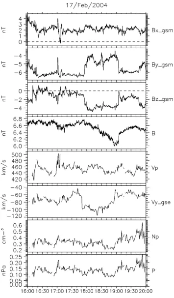
Fig. 1. 17 February 2004. From top to bottom: BX,BY andBZ
IMF components in the GSM frame as measured by ACE. Magnetic field magnitude as measured by ACE.
Solar wind velocity magnitude and Y component in he GSE frame as measured by ACE.
Density and dynamic pressure as measured by ACE.
The data have been shifted by 49 min to account for the propagation time from ACE to the Cluster spacecraft.
Research Letters (Tenuous Solar Wind, 2000). Studies per-formed during the 11 May event revealed several striking fea-tures. The magnetosphere had grown to exceptionally large dimensions due to the low solar wind pressure, about 100 times larger in volume than during average solar wind condi-tions (Lockwood et al., 2001). While the solar wind energy and density input to the magnetosphere was very low, Parks et al. (2000) showed that the auroral oval was still active and that the auroral activity was rather linked to the orientation of IMFBZ than to the solar wind density. Furthermore,
Tera-sawa et al. (2000) evidenced using Geotail data that the
plas-masheet and the magnetotail surprisingly maintained during this extremely low solar wind density period.
In this study, we will discuss a period when the solar wind density dropped to about 5% of its average value leading to a very low solar wind dynamic pressure (∼0.15 nPa). Dur-ing this event the Cluster spacecraft detect several high speed plasma jets at the inner edge of the magnetopause.
The presence of high speed plasma flows in this region of the magnetosphere is known to be a possible signature of magnetic reconnection between solar and magnetospheric magnetic field lines. Convincing experimental evidence has been given by in-situ observations in the magnetopause from the ISEE and AMPTE satellites (e.g. Paschmann et al., 1979; Sonnerup et al., 1981) to the most recent missions like Clus-ter (e.g. Bosqued et al., 2001; Bavassano-Cattaneo, 2006). Evidence for magnetic reconnection can be obtained both by fluid and kinetic considerations. They can give complemen-tary and independent information about the occurrence of magnetic reconnection. The fluid evidence consists of test-ing the tangential stress balance across the magnetopause. This test is named the Wal´en test (Hudson, 1970; Paschmann et al., 1979; Sonnerup et al., 1981). Kinetic evidence is given by the observation in the particle distribution function of transmitted magnetosheath ions with a D-shaped distribu-tion funcdistribu-tion and of reflected magnetosheath ions (Cowley, 1982).
In this paper, we will study the magnetopause and plasma jets properties in the frame of magnetic reconnection and dis-cuss the results in term of magnetospheric response to the extremely low solar wind density. We first start with a brief presentation of the instrumentation used for this study. Then, we describe the observations. In Sect. 3, we discuss the fluid properties of the magnetopause to evidence the robustness of magnetic reconnection. In Sect. 4, we study the ion dis-tribution function. It confirms the occurrence of magnetic reconnection and allows us to estimate the location of the re-connection site. Section 5 is dedicated to the study of the magnetopause motion and thickness. Section 6 summarizes the results and interpretations.
2 Instrumentation
The four identical Cluster satellites have been launched in 2000 on an elliptical orbit (4.0×19.6RE)with an inclination
of 90◦. A detailed description of the Cluster mission can be found in the paper of Escoubet et al. (2001).
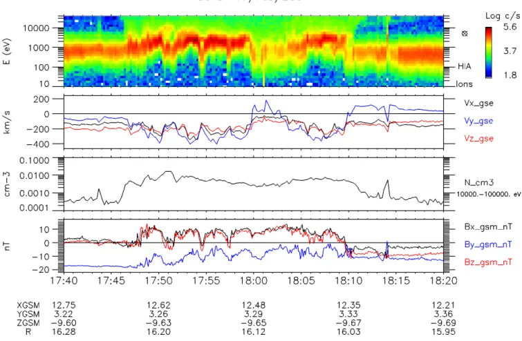
Fig. 2. Magnetic field and ion data from Cluster spacecraft 3 from 17:35 UT to 18:30 UT. From top to bottom: Energy-time spectrogram from HIA for all ions.
Ion velocity in the GSE frame computed from HIA.
Partial ion density for particles with energies higher than 10 keV computed from HIA. Magnetic filed components in the GSM frame computed from FGM.
In addition, we use high-resolution (5Hz) magnetic field data from the Cluster Fluxgate Magnetometers (FGM) (Balogh et al., 2001).
The ACE data are used to monitor the solar wind condi-tions. These data have been shifted in time to account for the solar wind propagation from ACE to the Cluster spacecraft.
3 Observations
From 15 February 2004, 20:00 UT to 18 February 2004, 01:00 UT, the solar wind density dropped to extremely low values (∼0.35 cm−3). In this study, we will focus on a time period taken on 17 February 2004 from 17:50 UT to 18:15 UT.
The Cluster satellites are located approximately in the (XZ)GSE plane in the Southern Hemisphere of the
dayside magnetosheath (SC4, 18:00 UT: XGSE=12.49RE,
YGSE=−0.72RE,ZGSE=−10.19RE)at a geocentric distance
of 16.14RE. The separation distance between the Cluster
spacecraft is around 500 km. During the considered time pe-riod the Cluster spacecraft are in the magnetosheath skim-ming the magnetopause. They are travelling in the direction of the magnetosphere where they enter after 21:00 UT.
The IMF, the solar wind density and velocity as given by the ACE spacecraft from 16:00 UT to 20:00 UT are presented in Fig. 1. These data have been time shifted by 49 min to ac-count for the solar wind propagation from ACE to Cluster. Before 19:00 UT the solar wind density is about 0.35 cm−3
and the dynamic pressure around 0.12 nPa. Then they slightly increase to reach respectively 0.5 cm−3and 0.17 nPa. The solar wind velocity, about 450 km/s, is almost constant during this time period. Due to its low density, the solar wind Alfv´en velocity is high (∼250 km/s) and the solar wind is only weakly super Alfv´enic (nA∼1.8). It is interesting to
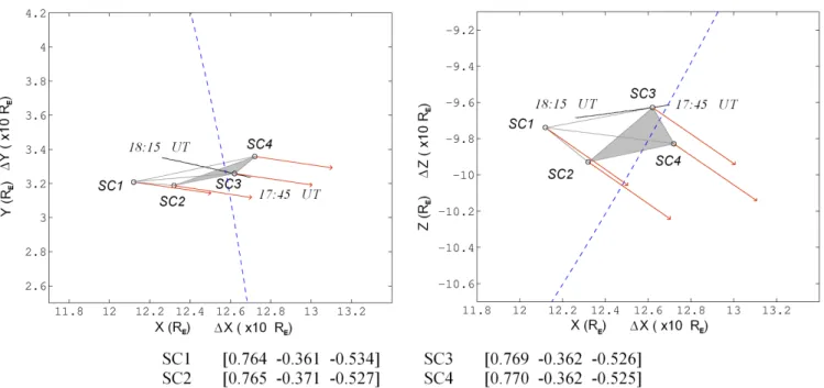
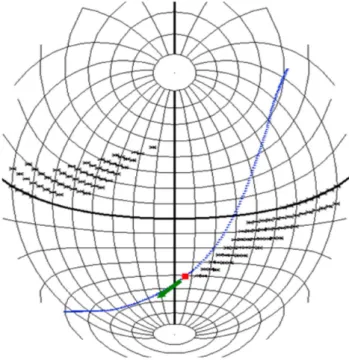
Fig. 3.Cluster spacecraft 3 orbit on 17 February 2004 from 17:45 UT to 18:15 UT projected in the X-Y (left) and X-Z (right) GSM planes (black line). The Cluster tetrahedron at 17:50 UT is also plotted. The separation distance between spacecraft has been multiplied by a factor of 10. The red arrows represent the components of the magnetopause normal predicted by the minimum variance analysis applied on magnetic field for each spacecraft. The blue dotted curve represents the magnetopause location as predicted by the Shue et al. (1997) model.
deviates from the sun-earth direction. According to ACE data, theYGSEcomponent of the solar wind velocity reaches −100 km/s. Just before 18:00 UT, the IMF turns from a dawnward orientation (BXGSM∼2 nT, BYGSM∼−6.5 nT, BZGSM∼−0.5 nT) to a dawnward/southward orientation
(BXGSM∼2.5 nT, BYGSM∼−4 nT, BZGSM∼−4 nT) with
al-most no variations ofBXGSM. This turning is accompanied
by a slow decrease of the total magnetic field strength from about 6.8 to 6.2 nT.
Cluster data from 17:40 UT to 18:20 UT are presented in Fig. 2. Until 17:46 UT, the Cluster spacecraft are lo-cated in the magnetosheath. The magnetic field mea-sured by the FGM instrument is mainly dawnward directed (BXGSM∼2 nT, BYGSM∼−17 nT,BZGSM∼0 nT) in a
direc-tion consistent with the IMF orientadirec-tion. The plasma has characteristic magnetosheath temperature (T i∼500 eV) and the ion velocity is mainly oriented in the southward/tailward direction as expected for magnetosheath plasma flowing around the magnetopause. However, the density (1 cm−3) is well below the usual magnetosheath density (∼25 cm−3) and the magnetosheath plasmaβis very low (0.15).
From 17:47 UT to 18:10 UT, a succession of magnetic field turnings is detected.BYGSMbecomes closer to 0 nT and BXGSMandBZGSMreach similar values around 10 nT. This
orientation is consistent with the expected magnetospheric field lines orientation at the Cluster location. These suc-cessive magnetic field rotations prove unambiguously that
the Cluster spacecraft cross the magnetopause several times during this time period. According to the magnetic field variations, Cluster magnetopause crossings occur quasi pe-riodically with a period of about 3–4 min. These periodic crossings are caused by large-scale oscillations of the mag-netopause probably triggered by solar wind pressure fluctu-ations (e.g. Sibeck et al., 1991). Due to the low separation distance between Cluster spacecraft, no information can be obtained on the propagation and wavelength of these tions. We just can state that the amplitude of these oscilla-tions is higher than the current layer thickness and that they are associated with a magnetopause motion at a velocity of about 20 km/s along the magnetopause normal (see Sect. 5). Simultaneously, the CIS experiment detects high-energy par-ticles (>10 keV) with a large amount of O+ ions, presum-ably of magnetospheric origin. These magnetospheric ions are also observed in the magnetosheath close to the magne-topause. Each of the magnetopause crossings is associated with the detection of high speed ion beams with velocities reaching 600 km/s. The flow speed enhancement across the magnetopause relative to the magnetosheath flow is higher than 300 km/s and accelerated plasma jets are oriented dawn-ward/southward/tailward. The peak of the flow speed always occurs at the magnetospheric side of the current layer.
IMF turning detected by ACE actually reached the Cluster spacecraft between 17:50 UT and 18:10 UT. However, it may have reached others regions of the dayside magnetopause be-fore Cluster observation of theBZ turning. This magnetic
field reversal created favourable conditions for magnetic re-connection at the dayside magnetopause.
4 Evidence for magnetic reconnection
In this section, we discuss the properties magnetopause and of the accelerated ion beams to show fluid and kinetic evi-dence for magnetic reconnection.
4.1 Magnetopause orientation
As a first step, we performed a variance analysis on magnetic field data for each Cluster spacecraft respectively for the full time interval (17:47 UT to 18:11 UT) and for each individ-ual crossing to determine the magnetopause orientation. The normal orientation obtained for each spacecraft and for each time interval is very similar with differences of a few degrees, not meaningful as it is comparable with the uncertainty asso-ciated with this method.
Figure 3 presents a projection of the magnetopause normal vector obtained by the minimum variance analysis for the full time interval respectively in the(XY )GSMand(XZ)GSM
planes. The location and orientation of the magnetopause are compared with an interpolation of the Shue et al. (1997) mag-netopause model. Whereas this model is defined for solar wind dynamic pressures higher than 0.5 nPa, we interpolated it for a dynamic pressure of 0.15 nPa. Both magnetopause location and orientation obtained with this model are in good agreement with Cluster data. However, the magnetopause orientation in the(XY )GSE plane obtained by the minimum
variance analysis on Cluster magnetic field data slightly dif-fers with the magnetopause orientation given by the Shue et al. model. This is possibly an effect of the azimuthal com-ponent of the solar wind (VYGSE∼−100 km/s) that slightly
distort the magnetopause, shifting its nose in the +YGSE
di-rection. Note that, according to the Shue et al. (1997) magne-topause model, the magnemagne-topause extends at a radial distance of about 16REat the subsolar point.
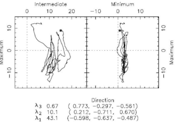
Then we projected the magnetic field on the magnetopause frame, using the magnetopause orientation given by the min-imum variance analysis. This is exemplified in Fig. 4 which presents the hodogram obtained with spacecraft 3 magnetic field data for the whole time interval, from 17:47 UT to 18:11 UT. It clearly evidences a rotation of about 90◦ of the magnetic field in the magnetopause plane for each netopause crossing (left panel) and the presence of a mag-netic field along the magnetopause normal (right panel). The eigenvaluesλ1, λ2andλ3of the magnetic variance matrix
are also indicated. They fulfil quite satisfactorily the
condi-Fig. 4. Magnetic field hodogram obtained by minimum vari-ance analysis applied on Cluster 3 magnetic field data between 17:47:00 UT and 18:11:00 UT. The left pane represents the projec-tion of the magnetic field in the plane containing the maximum and intermediate variance axis, i.e. in the magnetopause plane. The left panel represents the projection of the magnetic field in the plane containing the minimum and maximum variance axis. The compo-nents in the GSE a plane of respectively the minimum, intermediate and maximum variance axis are given in the bottom of this figure.
tionλ1,λ2≫λ3required to have a reliable estimation of the
magnetopause normal.
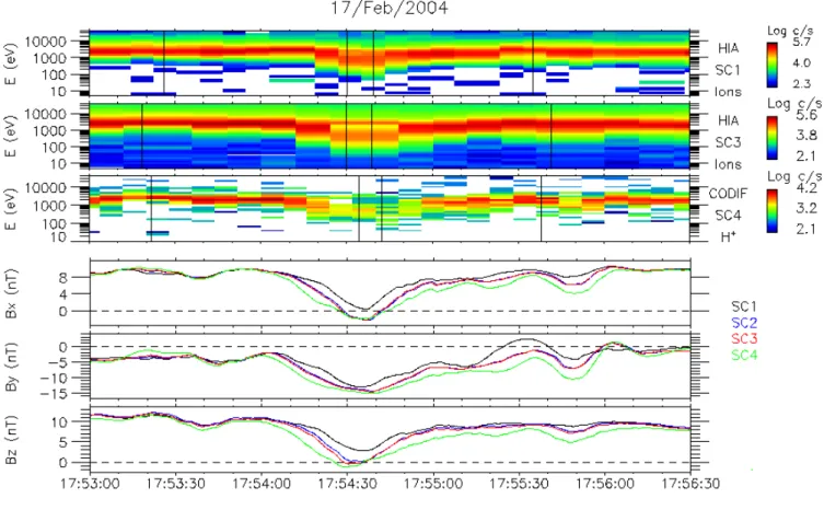
Fig. 5.17 February 2004 from 17:53 UT to 17:56:30 UT. From top to bottom: Energy-time spectrogram from HIA for all ions, spacecraft 1.
Energy-time spectrogram from HIA for all ions, spacecraft 3. Energy-time spectrogram from CODIF for O+ions, spacecraft 4.
Magnetic fieldBXcomponent in the GSE frame for the 4 Cluster spacecraft for Cluster 1 (black), Cluster 2 (blue), Cluster 3 (red) and
Cluster 4 (green) computed from FGM data. Magnetic fieldBY component in the GSE frame for the 4 Cluster spacecraft with the same colour code computed from FGM data. Magnetic fieldBZcomponent in the GSE frame for the 4 Cluster with the same colour code spacecraft
computed from FGM data.
however the Fig. 4 evidences that we do not obtain an accu-rate result.
Furthermore it must be stressed that, although low (≪180◦), the local magnetic shear can not be used to evalu-ate the validity of component or anti-parallel reconnection as the reconnection site may be far from the Cluster spacecraft (see below).
4.2 DeHoffmann-Teller analysis and Wal´en test
In this part, we discuss in more detail two consecutive mag-netopause crossings, chosen arbitrarily, respectively from the magnetosphere to the magnetosheath and from the magne-tosheath to the magnetosphere. The results obtained for the other magnetopause crossings are similar. Figure 5 presents Cluster data during these two crossings. Cluster spacecraft are first located in the magnetospheric boundary layer char-acterized by the presence of accelerated ion beams and by a magnetic field with a magnetospheric orientation. Around
17:54:30 UT the spacecraft enter briefly the magnetosheath and then return to the boundary layer.
Magnetohydrodynamic models for 1-dimensional steady state reconnection predict that the flow is Alfv´enic in the deHoffmann-Teller (dHT) frame of reference (Hudson, 1970). We will use the tangential stress balance to examine the occurrence of Alfv´enic flow acceleration. The time in-tervals used to check the tangential stress balance for each spacecraft are indicated by vertical lines in Fig. 5.
The first step consists to search for the existence of a well-defined dHT frame for each spacecraft. In this frame, moving with a velocityVH T along the presumed rotational
disconti-nuity, the electric field vanishes. To obtain this frame we will use the method described in detail by Khrabrov and Son-nerup (1998). TheVH T velocity is obtained by minimizing
the quantity:
D=X
m
Vm−VH T
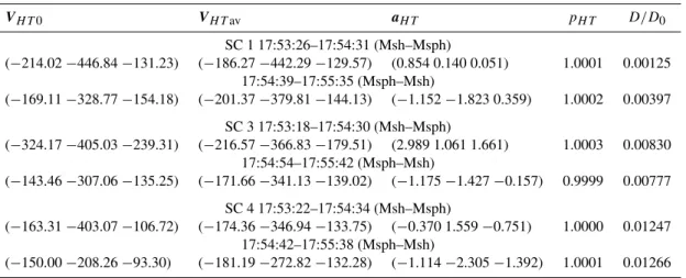
Table 1.dHT analysis results for the two consecutive magnetopause crossings discussed in detail in this section. Velocities are in km/s and acceleration in km/s2. All vectors are expressed in the GSE frame. The results presented here have been obtained by introducing a constant acceleration of the dHT frame: VH T=VH T0+aH Tt. pH T is the fitting slope betweenEH T=−VH T×BandEC=−V×B, the convection electric field.D/D0is the least square quality factor.VH Tavis the average velocity of the dHT frame.
VH T0 VH Tav aH T pH T D/D0
SC 1 17:53:26–17:54:31 (Msh–Msph)
(−214.02−446.84−131.23) (−186.27−442.29−129.57) (0.854 0.140 0.051) 1.0001 0.00125 17:54:39–17:55:35 (Msph–Msh)
(−169.11−328.77−154.18) (−201.37−379.81−144.13) (−1.152−1.823 0.359) 1.0002 0.00397
SC 3 17:53:18–17:54:30 (Msh–Msph)
(−324.17−405.03−239.31) (−216.57−366.83−179.51) (2.989 1.061 1.661) 1.0003 0.00830 17:54:54–17:55:42 (Msph–Msh)
(−143.46−307.06−135.25) (−171.66−341.13−139.02) (−1.175−1.427−0.157) 0.9999 0.00777
SC 4 17:53:22–17:54:34 (Msh–Msph)
(−163.31−403.07−106.72) (−174.36−346.94−133.75) (−0.370 1.559−0.751) 1.0000 0.01247 17:54:42–17:55:38 (Msph–Msh)
(−150.00−208.26−93.30) (−181.19−272.82−132.28) (−1.114−2.305−1.392) 1.0001 0.01266
using the measured magnetic field (Bm) and ion velocity (Vm) during the discontinuity crossing. This method can be improved by choosing a dHT frame continuously accel-erated (VH T=VH T0+aH Tt) instead of a dHT frame moving at a constant velocity.
Both methods have been used. The results are compa-rable although the dHT frame velocities obtained with the accelerated frame are more similar from one spacecraft to another (Table 1). There is a very strong correlation between EH T=−VH T×Band the convection electric field, with fit-ting slopes very close to 1 and very small least-squares resid-uals. We can thus conclude that for each spacecraft a well-defined dHT frame exists. This frame is mainly moving along the magnetopause at an average velocity of 430 km/s in the dawnward/southward/tailward direction. Its velocity along the magnetopause normal (about tens of km/s) corre-sponds to the magnetopause motion along its normal and will be discussed later on.
The second step is the tangential stress balance or Wal´en test (Hudson, 1970; Paschmann et al., 1979; Sonnerup et al., 1981). It consists of checking if the plasma is Alfv´enic in the dHT frame across the discontinuity, i.e. if:
V−VH T = ±VA (2)
The sign + is for a reconnection site located southward and the sign – for a reconnection site located northward.Vis the plasma velocity,VH T the dHT frame velocity and VA the Alfv´en velocity given by:
VA=B
1−α µ0ρ
1/2
(3)
where
α=(ρ//−ρ⊥) µ0
B2 (4)
is the anisotropy factor.
The results of this test, given in Table 2, present the fitting slopes between the plasma velocity in the dHT frame and the Alfv´en velocity obtained using a component-by-component scatter plot of these velocities. The corresponding correlation coefficient is also indicated. These two velocities are well correlated but the plasma velocity in the dHT frame is only 46 to 62 percent of the Alfv´en velocity.
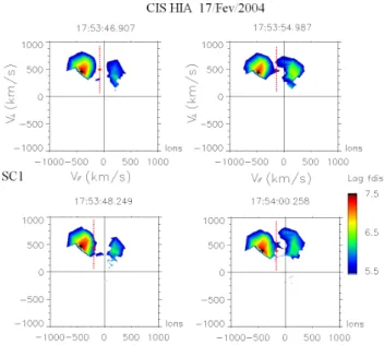
Fig. 6.17 February 2004. Bi-dimensional cut-off of the ion distri-bution function in the Vper-Vpar plane for spacecraft 1 (top pan-els) and spacecraft 3 (bottom panel) from HIA instrument. The red cross represent the velocity of the deHoffmann-Teller frame and the black cross the velocity of the main ion population. Note that the ion distribution function of the transmitted ion population is trun-cated because of the operating mode of the HIA instrument.
only detected variation at that time is a decrease of theVYGSE
velocity from about 100 km/s to 0 km/s with no notable mod-ification of the other components. It is more difficult to es-timate the error during the measurement of ion beams as the ion velocity is quickly changing. We used Whisper plasma frequency measurement to estimate this error. Unfortunately this indirect measurement of the plasma density is perturbed by the presence of large band emissions (P. Canu, private communication). This measurement has thus a big uncer-tainty. For example, with Whisper we obtain a density com-prised between 1 and 1.6 cm−3at 18:00 TU whereas the HIA
instrument gives a density of 0.65 cm−3. It is thus difficult to
obtain a precise corrective coefficient in the magnetopause boundary layer. However, the density underestimation can be roughly estimated as being close to two in this region too. This underestimation of the density leads to an overesti-mation of the Alfv´en velocity of a factor of about√2. Fur-thermore, the Alfv´en velocity has been computed consider-ing that the pressure anisotropyαwas null because it is im-possible to determine it accurately. Indeed, the inadequate operating mode of the CIS experiment leads to an incomplete sampling of the ion distribution function and causes errors in the computation of the perpendicular and parallel tempera-tures. This assumption can also affect in a lower degree the result of the Wal´en test.
After correcting the density, the ion velocity in the dHT frame is about 0.7 to 0.9VA, which constitutes a
satisfy-ing result for the Wal´en test (Khrabov et Sonnerup, 1998). Indeed, while the directional change of the plasma veloc-ity is generally in good agreement with the Alfv´en velocveloc-ity, the magnitude of the velocity change is usually smaller than the Alfv´en speed. The good correlation coefficient of the component-by-component scatter plot and the smaller than VA plasma velocity reveal a similar behaviour in this event.
The cause of this discrepancy is not understood yet but sev-eral explanations have been proposed (Paschmann and Son-nerup, 2008). This includes among other things the under-estimation of the density due to the presence of cold parti-cle populations, two- or three-dimensional effects and non-gyrotropic plasma behaviour.
The plasma flow in the dHT frame is oppositely directed to the magnetic field as evidenced by the negative sign ofpW a.
It corresponds to a reconnection site located northward of the satellite, in agreement with the orientation of the magnetic field along the magnetopause normal.
4.3 Ion distribution function
The last step to reveal the reconnection process is to examine the ion distribution function. In particular, one of the most important kinetic signatures of the reconnection process is the presence of D-shaped distribution functions as predicted by the reconnection theory. Indeed, in the dHT frame, only the particles with positive (northward of the reconnection site) or negative (southward of the reconnection site) veloc-ities along the magnetic field can be transmitted through the magnetopause (Cowley et al., 1982). In a fixed frame, it in-duces a cutoff of the ion distribution function atVH T along
the magnetic field and therefore the ion distribution function must exhibit a D-shape (e.g. Gosling et al., 1991; Fuselier et al., 2000; Phan et al., 1996).
Two consecutive slices of the ion distribution function in the (VPAR–VPERP)frame obtained with the Cluster 1 and 3
HIA instruments for the accelerated flows at∼17:54 UT are given in Fig. 6. These distribution functions, almost identical for the two spacecraft, show the presence of two ion popula-tions.
The first one, with a negative velocity along the magnetic field, corresponds to the H+ magnetosheath ions transmit-ted through the magnetopause. The distribution function is truncated in its lower part due to the inadequate operating mode of the HIA instrument. It distorts slightly the ion dis-tribution function and makes difficult the identification of the predicted D-shape. However, we clearly see a cut-off of the parallel velocities atVH T.
The second population is flowing in the magnetic field di-rection. It consists of magnetosheath ions, which have pen-etrated into the magnetosphere and then have been reflected by the magnetic mirror force at low altitude.
Table 2. Wal´en test results for the two consecutive magnetopause crossings discussed in detail in this section. pW arepresents the fitting
slope of (V–VH T)versusVAandcW athe corresponding correlation coefficient. The last column indicates the value ofpW aafter correction
of the density. These results don’t take into account the density correction due to the inadequate operating mode of the CIS experiment.
pWa cWa corrected pWa
Satellite 1 17:53:26–17:54:31 (Msh–Msph) −0.5926 0.9632 −0,8380 17:54:39–17:55:35 (Msph–Msh) −0.4849 0.9468 −0.6857
Satellite 3 17:53:18–17:54:30 (Msh–Msph) −0.5790 0.9614 −0.8188 17:54:30–17:55:42 (Msph–Msh) −0.4609 0.9576 −0.6518
Satellite 4 17:53:22–17:54:34 (Msh–Msph) −0.5543 0.9359 −0.7838 17:54:42–17:55:38 (Msph–Msh) −0.6214 0.9708 −0.8787
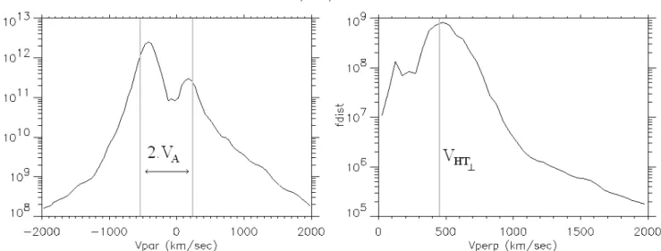
Fig. 7.17 February 2004, 17:53:48.289 UT. Ion distribution function with respect to their velocity parallel to the magnetic field (left panel) and to their velocity perpendicular to the magnetic field (right panel) from SC3 HIA instrument. In the left panel, the two vertical lines represent respectively the component parallel to the magnetic field ofVH T–VAandVH T+VA. In the right panel the vertical line represents
the component of the dHT velocity perpendicular to the magnetic field.
(Cowley, 1982) and observed, in particular at high latitude near the cusp region (e.g. Fuselier et al., 2000). However this is to our knowledge the first observation of a reflected ion population in the dayside magnetopause at such a high geocentric distance. Figure 7 displays the ion distribution function with respect to the parallel and perpendicular ve-locity measured by SC3 at 17:53:48 UT. In the direction per-pendicular to the magnetic field, only one peak is observed atVH T⊥. On the contrary, in the magnetic field direction, we clearly observe two peaks. The first one, atVH T //–VA
corresponds to the transmitted ions and the second one at VH T //+VA corresponds to the reflected ions. According to
the theory, the reflected and transmitted populations are flow-ing at respectively +VAand−VAin the dHT frame.
Previous studies reported the presence of low speed cut-offs of the transmitted and reflected populations. Interpreted
as a velocity filter effect caused by the convection of the re-connected field line, they have been used to estimate the lo-cation of the X-line (e.g. Fuselier et al., 2000). In particular, a low speed cut off is expected to be observed on the mirrored population if the spacecraft is not too far from the reconnec-tion region. Indeed, only particles with a sufficient parallel velocity have time to be mirrored and reach the spacecraft during the time the reconnected field line is convected from the X-line to the spacecraft. In this event, the absence of ve-locity cut off means that Cluster spacecraft are far from the reconnection site. Thus, we can not use this method to esti-mate the location of the X-line.
Fig. 8. Front view of the magnetopause. The red cross represents the location of Cluster spacecraft at 18:00 UT. The blue line repre-sents the IMF line passing by Cluster spacecraft. The regions in-dicated by black crosses are regions of high magnetic shear where antiparallel reconnection models expect reconnection to occur. The green arrow indicated the direction of convection at Cluster location as obtained by the dHT analysis. The reconnection site is estimated to lie in a region located in the opposite direction of the convection velocity at some tens ofREfrom Cluster spacecraft.
field model. Supposing that the transmitted ions are re-flected close to the earth, the distance they travelled to go from their entrance site in the magnetosphere to their mir-ror point and then to come back to Cluster spacecraft is of about 2×19=38RE. Because these ions travel along the
magnetic field lines at the Alfv´en velocity (∼350–400 km/s), their travel time is estimated around (38×6378)/400=600 s or 10 min. During that time, the reconnected magnetic field lines are convected along the magnetopause. From the dHT frame velocity in the magnetopause plane (or equivalently from the ion perpendicular velocity) we estimate the convec-tion velocity to be approximately 400 km/s. Therefore, the reconnection site may be located at a distance higher than 600×400=240 000 km or 38RE from the observation point.
Obviously, this is a rough estimation of the location of the X-line. However, we can state that the observation of a re-flected population at such a high geocentric distance implies that the Cluster spacecraft are located at several tens ofRE
from the merging region. This very high distance has to be considered taking into account the large size of the magneto-sphere during this time period. Furthermore, according to the direction of the dHT velocity (on average in the GSM frame: VH T X=−188 km/s, VH T Y=−273 km/s, VH T Z=−269 km/s),
we estimate that the reconnection site may be located in the duskward side of the dayside magnetopause. As shown by a mapping of IMF magnetic field line on the magnetopause, the magnetic shear across the magnetopause is high in this region. This seems consistent with antiparallel reconnection model predictions of the X-line location for the correspond-ing IMF conditions (Fig. 8). However, due to low precision in the determination of the location of the X-line, we can-not claim that the antiparallel reconnection model better de-scribes the large scale configuration of magnetic reconnec-tion than component reconnecreconnec-tion during this event.
Another information is deduced from the presence of the reflected population. The reflected ions are detected during every magnetopause crossing, in particular during the first one at around 17:50 UT (not shown). As a consequence, the reconnection process must have started at least 10 min be-fore 17:50 UT, the time for magnetosheath ions to enter the magnetosphere, be reflected and reach the Cluster spacecraft. We conclude that the reconnection onset must have occurred before 17:40 UT.
5 Magnetopause motion and thickness
Finally, we turn to an evaluation of the motion and thickness of the magnetopause with two different methods (Table 3).
We first made a multi-spacecraft analysis to estimate the magnetopause motion along its normal. We use the time de-lays for the magnetopause crossings between different Clus-ter spacecraft obtained with high-resolution magnetic field data (5 Hz). The magnetopause is assumed to be a planar surface, which may be a valuable assumption due to the low separation distance between Cluster spacecraft during this event. From the plasma and magnetic field measurements, we expect an inward motion for the first magnetopause cross-ing and an outward motion for the second one. We obtain a magnetopause velocity comprised between−19.5 km/s and −26.4 km/s and between 17.5 km/s and 22.3 km/s, respec-tively, for the inward and outward motion. Note that we did not use the Cluster 2 spacecraft as its separation distance from the Cluster 3 spacecraft along the magnetopause normal is too short.
The second method consists of a single spacecraft analy-sis. Here, the magnetopause motion along its normal is eval-uated by projecting the dHT velocity along the magnetopause normal. The velocities are comprised between−44.5 km/s and−69.4 km/s and between−1.6 km/s and 23.8 km/s, re-spectively, for the first and second crossing. This method gives more variable results because of its high sensitivity to the magnetopause normal orientation (Khrabov and Son-nerup, 1998) and must be less reliable than the time delay analysis.
For the first magnetopause crossing, from the magneto-sphere to the magnetosheath, the magnetic fields measured by SC3 and SC4 at the beginning and at the end of the crossing are similar while they are separated in the direction normal to the magnetopause. It indicates that these two satel-lites are located in regions where the magnetic field is almost uniform and thus that they have crossed the magnetopause current layer almost entirely. On the contrary, the magnetic field variations detected by SC1 are less pronounced than those detected by the other Cluster spacecraft. This space-craft, which is the closest to the earth, has only partially crossed the current sheet and will not be used to estimate its thickness.
The magnetic field rotation during this crossing lasts 35 s for SC3 and 40 s for SC4. The magnetopause thickness is thus estimated between 23×35∼800 km and 23×40∼900 km. For the second crossing, the magnetic field fluctuations (in particular in theYGSE direction) make
diffi-cult this kind of analysis.
We made a similar analysis for the other magnetopause crossings and obtained comparable results. These values are compatible with those obtained during standard solar wind conditions with ISEE spacecraft at similar latitudes: 10– 80 km/s for the magnetopause velocity and 400–1000 km for the magnetopause thickness (Berchem and Russel, 1982). However we would expect a thicker magnetopause during this event as the ion gyroradii is about three times higher than during nominal solar wind conditions due to the low magnetic field value. Indeed, the magnetopause thickness, corresponding to 3 protons gyroradii is lower than the aver-age value of 10 gyroradii obtained by Berchem and Russell (1982) albeit it is in the range of values obtained in their sta-tistical study.
6 Conclusion
We have presented in-situ measurements taken in the magne-tosheath/magnetopause during exceptional conditions when the solar wind almost disappeared. Due to the low solar wind density, the magnetosheath beta was very low (0.15) and the magnetosphere was dilated and extended up to 16RE in the
solar direction.
Between 17:50 UT and 18:10 UT Cluster spacecraft cross several times the magnetopause and each of these crossings is associated with the presence of high velocity plasma jets.
We showed the presence of a magnetic field of a few nT along the magnetopause normal. We also evidenced that the tangential stress balance was satisfied. The analysis of the ion distribution function revealed the presence of D-shaped ion distribution functions and of a reflected ion population. Both fluid and kinetic considerations are consistent and ev-idence that the high velocity plasma jets result from recon-nection in the dayside magnetopause.
Table 3.Magnetopause velocity in km/s deduced from the time de-lays between different spacecraft crossings and from the projection of the dHT velocity along the magnetopause normal.
Satellites Msh-Msph Msph-Msh
Multi spacecraft analysis
1–3 −26.4 22.3 1–4 −23.2 20.1 3–4 −19.5 17.5
VH Tn
1 −44.5 −1.6 3 −51.3 23.8 4 −69.4 15.2
Inside the plasma jets, the Cluster spacecraft simultane-ously detect reflected ions. This is the first time to our knowl-edge that reflected ions are observed at such a high geocentric distance. Because of this large distance, the time of flight of these ions is important (about 10 min). It implies that the re-connection site is located at several tens of Earth radii from Cluster spacecraft. The direction of the magnetic field lines convection at the Cluster location suggests that the reconnec-tion site is probably located in the dusk side of the dayside magnetopause.
This reflected population also indicates that reconnection started 10 min before the Cluster spacecraft detect the accel-erated plasma jets (from about 17:50 UT to 18:10 UT). We interpret it as an evidence for continuous reconnection dur-ing more than half an hour. However, we cannot totally ex-clude that the reconnection process ceases between the jets when the Cluster spacecraft are located in the magnetosheath but the systematic observation of plasma jets at each magne-topause crossing strongly indicates continuous reconnection. Cluster magnetic field measurements reveal that a south-ward turning of the IMF reached the Cluster spacecraft be-tween 17:50 UT and 18:10 UT. However, it may have reached other regions of the magnetopause before that time. Because the X component of the IMF is low, the southward turn-ing must have reached the subsolar point before the Clus-ter spacecraft. The separation distance between the subso-lar point and the Cluster spacecraft along theXGSE axis is
of about 16–12.5=3.5RE. Taking a propagation speed into
These observations tend to show that during this period of low solar wind density, magnetic reconnection was effi-cient and provided solar wind plasma to the magnetosphere. This is consistent with statistical study of accelerated flows at the magnetopause (Scurry et al., 1994a, b) which revealed that the merging process depends on the local magnetosheath beta. According to this study, the lower is the magnetosheath beta, the higher is the probability to observe accelerated flows at the magnetopause.
Furthermore, when the solar wind dynamic pressure is very low as during this event, the magnetosphere is extremely dilated and its cross section with the solar wind is high. The size of the region where solar wind plasma penetrates into the magnetosphere via magnetic reconnection must therefore be more extended than during standard conditions.
Because of its possible increased efficiency and because of the dilatation of the magnetosphere, magnetic reconnec-tion may be more efficient to provide solar wind plasma to the magnetosphere during periods of low solar wind den-sity. It can partially compensate the low density of the solar wind source. This could explain why during prolonged (a few days) periods of low solar wind density, the plasmasheet and magnetotail are maintained (Terasawa et al., 2000).
Finally, we also showed that the magnetopause thickness (∼800 km) and velocity (∼20 km/s) do not differ from the average values given by statistical studies (e.g. Berchem and Russell, 1982) and that, while the magnetosphere is ex-tremely extended, its location is still well predicted by the Shue et al. (1997) magnetopause model.
Acknowledgements. We thank the principal investigators of ACE MAG and SWEPAM experiments for making their data avaible.
The authors are grateful to E. Penou for the development of the Cluster CIS software. R. Maggiolo thanks M. Roth for helpful dis-cussion and comments.
Topical Editor I. A. Daglis thanks J. De Keyser and A. V. Dmitriev for their help in evaluating this paper.
References
Arnoldy, R. L.: Signature in the interplanetary medium for sub-storms, J. Geophys. Res., 76, 5189–5201, 1971.
Balogh, A., Carr, C. M., Acu˜na, M. H., Dunlop, M. W., Beek, T. J., Brown, P., Fornac¸on, H., Georgescu, E., Glassmeier, K.-H., Harris, J., Musmann, G., Oddy, T., and Schwingenschuh, K.: The Cluster Magnetic Field Investigation: overview of in-flight performance and initial results, Ann. Geophys., 19, 1207–1217, 2001, http://www.ann-geophys.net/19/1207/2001/.
Bavassano Cattaneo, M. B., Marcucci, M. F., Retin`o, A., Pallocchia, G., R`eme, H., Dandouras, I., Kistler, L. M., Klecker, B., Carlson, C. W., Korth, A., McCarthy, M., Lundin, R., and Balogh, A.: Kinetic signatures during a quasi-continuous lobe reconnection event: Cluster Ion Spectrometer (CIS) observations, J. Geophys. Res., 111, 9212, doi:10.1029/2006JA011623, 2006.
Berchem, J. and Russell, C. T.: The thickness of the magnetopause current layer – ISEE 1 and 2 observations, J. Geophys. Res., 87, 2108–2114, 1982.
Bosqued, J. M., Phan, T. D., Dandouras, I., Escoubet, C. P., R`eme, H., Balogh, A., Dunlop, M. W., Alcayd´e, D., Amata, E., Bavassano-Cattaneo, M.-B., Bruno, R., Carlson, C., DiLellis, A. M., Eliasson, L., Formisano, V., Kistler, L. M., Klecker, B., Ko-rth, A., Kucharek, H., Lundin, R., McCarthy, M., McFadden, J. P., M¨obius, E., Parks, G. K., and Sauvaud, J.-A.: Cluster observa-tions of the high-latitude magnetopause and cusp: initial results from the CIS ion instruments, Ann. Geophys., 19, 1545–1566, 2001, http://www.ann-geophys.net/19/1545/2001/.
Cowley, S. W. H.: The causes of convection in the earth’s magne-tosphere -A review of developments during the IMS, Rev. Geo-phys. Space Phys., 20, 531–565, 1982.
Escoubet, C. P., Fehringer, M., and Goldstein, M.: The Cluster mis-sion, Ann. Geophys., 19, 1197–1200, 2001,
http://www.ann-geophys.net/19/1197/2001/.
Fuselier, S. A., Trattner, K. J., and Petrinec, S. M.: Cusp observation of high- and low-latitude reconnection for northward interplane-tary magnetic field, J. Geophys. Res., 105, 253–266, 2000. Gosling, J. T., Thomsen, M. F., Bame, S. J., Elphic, R. C., and
Russell, C. T.: Observations of reconnection of interplanetary and lobe magnetic field lines at the high-latitude magnetopause, J. Geophys. Res., 96, 14 097–14 106, 1991.
Hudson, P. D.: Discontinuities in an anisotropic plasma and their identification in the solar wind, Planet. Space Sci., 18, 1611– 1622, 1970.
Janardhan, P., Fujiki, K., Sawant, H. S., Kojima, M., Hakamada, K., and Krishnan, R.: Source regions of solar wind disappearance events, J. Geophys. Res., 113, 3102–3110, 2008.
Khrabrov, A. V. and Sonnerup, B. O.: DeHoffmann-Teller analy-sis. Analysis Methods for Multi-Spacecraft Data, ISSI Scientific Report SR-001, ESA Pub. Div., 221, 221–248, 1998.
Lockwood, M.: Astronomy: the day the solar wind nearly died, Nature, 409(6821), 677–679, 2001.
Parks, G., Brittnacher, M., Chua, D., Fillingim, M., Germany, G., and Spann, J.: Behaviour of the aurora during 10–12 May, 1999 when the solar wind nearly disappeared, Geophys. Res. Lett., 27, 4033–4036, 2000.
Paschmann, G., Sonnerup, B. U. O., Papamastorakis, I., Sckopke, N., Haerendel, G., Bame, S. J., Asbridge, J. R., Gosling, J. T., Russell, C. T., and Elphic, R. C.: Plasma acceleration at the Earth’s magnetopause, Evidence for magnetic reconnection, Na-ture, 282, 243–246, 1979.
Paschmann, G. and Sonnerup, B. O.: DeHoffmann-Teller analysis. Analysis Methods for Multi-Spacecraft Data, ISSI Scientific Re-port SR-008, ESA Pub. Div., 65, 65–74, 2008.
Phan, T. D., Paschmann, G., and Sonnerup, B. U. O.: Low-latitude dayside magnetopause and boundary layer for high magnetic shear 2. Occurrence of magnetic reconnection, J. Geophys. Res., 101, 7871–7828, 1996.
R`eme, H., Aoustin, C., Bosqued, J. M., et al.: First multispacecraft ion measurements in and near the earth’s magnetosphere with the identical Cluster Ion Spectrometry (CIS) Experiment, Ann. Geophys., 19, 1303–1354, 2001,
http://www.ann-geophys.net/19/1303/2001/.
Scurry, L., Russell, C. T., and Gosling, J. T.: Geomagnetic activity and beta dependence of the dayside reconnection rate, J. Geo-phys. Res., 99, 14 811–14 814, 1994a.
Res., 99, 14 815–14 829, 1994b.
Shue, J.-H., Chao, J. K., Fu, H. C., Russell, C. T., Song, P., Khurana, K. K., and Singer, H. J.: A new functional form to study the solar wind control of the magnetopause size and shape, J. Geophys. Res., 102, 9497–9512, 1997.
Sibeck, D. G., Lopez, R. E., and Roelof, E. C.: Solar wind control of the magnetopause shape, location and motion, J. Geophys. Res., 96, 5489–5495, 1991.
Sonnerup, B. U. O., Paschmann, G., Papamastorakis, I., Sckopke, N., Haerendel, G., Bame, S. J., Asbridge, J. R., Gosling, J. T., and Russell, C. T.: Evidence for magnetic reconnection at the Earth’s magnetopause, J. Geophys. Res., 86, 10 049–10 067, 1981.
Spreiter, J. R. and Stahara, S. S.: A new predictive model for de-termining solar wind-terrestrial planet interactions, J. Geophys. Res., 85, 6769–6777, 1980.
Tenuous solar wind: Special issue, Geophys. Res. Lett., 27, 3761– 3792, 2000.