Fields of study and the earnings gap by race in Brazil

(1)

Todos os direitos reservados.

É proibida a reprodução parcial ou integral do conteúdo

deste documento por qualquer meio de distribuição, digital ou

impresso, sem a expressa autorização do

REAP ou de seu autor.

Fields of study and

the earnings gap by race in Brazil

Mauricio Reis

(2)

FIELDS OF STUDY AND THE EARNINGS GAP BY RACE IN BRAZIL

Mauricio Reis

Instituto de Pesquisa Econômica Aplicada (IPEA) Av. Presidente Antonio Carlos, 51(1409)

(3)

1

Fields of study and the earnings gap by race in Brazil

1

Mauricio Reis

Instituto de Pesquisa Economica Aplicada

Av. Presidente Antonio Carlos, 51(1409)

Rio de Janeiro, RJ, Brazil – 20020-010

(5521)3515-8586

Fax: (5521)3515-8547

mauricio.reis@ipea.gov.br

Abstract

The labor earnings differential by race in Brazil is high even among individuals who

completed at least a bachelor’s degree. Decompositions of the earnings gap between

white and black workers using the 2000 and 2010 Census data indicate that disparities

in the distributions of racial groups across fields of study help explain 14% of the total

mean earnings differential in 2000 and 24% in 2010. The estimated contribution of this

factor seems to be larger at the median of the earnings distribution, accounting for one

third of the gap between white and black workers in 2010.

JEL: J15, J31, I20.

Keywords: Field of study, race, labor earnings gap.

1

This paper has benefited from many helpful comments and suggestions from Paola Salardi and

participants at the IARIW-IBGE Conference on Income, Wealth and Well-being in Latin America (Rio de

(4)

2

1 – Introduction

The earnings difference between white and black workers is noticeably high in

Brazil, and disparities in the schooling level by race help to explain an important part of

this earnings gap. The average educational level of black individuals improved over

time, as well as the proportion of blacks who reached tertiary or higher educational

level. In 2000, black workers represented 15% of the Brazilian labor force with a

bachelor’s or graduate degree, whereas in 2010 the participation of this racial group

increased to 25%.2 This educational improvement contributed to important earnings

gains for many black individuals, who entered a select group that comprised 15% of the

Brazilian labor force in 2010. Workers with at least a bachelor’s degree in Brazil earn

three times more than those with a lower level of schooling, on average.

Although the attainment of a bachelor’s or graduate degree by a black worker

usually provides important benefits at the individual level, it does not assure equal labor

market outcomes compared to white workers with the same level of education.

Empirical evidence shows that whites earned 39% more per hour than blacks among

Brazilian workers with at least a bachelor’s degree in 2000, while in 2010 the hourly

labor earnings differential between whites and blacks increased to 41%.

An aspect that draws attention when comparing white and black individuals with

tertiary education in Brazil is the unequal distribution across fields of study. Black

workers are more concentrated in areas like education, arts, humanities and languages,

and social care, while white individuals are more represented in engineering and health

professions. Several studies present evidence for different countries indicating that

university premium varies substantially by field of study.3 The Brazilian labor market

not only exhibits important earnings differences across fields of study, but also the

participation of black individuals is much higher in fields of study with lower average

earnings. In both 2000 and 2010, for example, the average labor earnings in engineering

are three times higher than that in education. Thus, the distributions of white and black

workers with tertiary education across fields of study may play a role in the labor

earnings gap by race in Brazil. It should be mentioned that there are many other

elements that may contribute to explaining this earnings differential by race in Brazil,

2

According to Census data, only 3.7% of the black workers in Brazil had at least a bachelor’s degree in 2000, while 8.5% reached this level of schooling in 2010. In the latter period, 22.2% of the white workers

had a bachelor’s or graduate degree.

3

(5)

3

such as demographic characteristics, mismatch between field of education and

occupation, proportion of workers with a graduate degree, as well as unobserved

variables, like discrimination and quality of education.

The aim of this paper is to investigate the labor earnings differential between

white and black workers with a bachelor’s or graduate degree in Brazil, decomposing

this gap into components accounted for by observable differences across individuals,

and differences in the return on these characteristics. The empirical analysis uses data

from the 2000 and 2010 Brazilian Census. This survey, conducted by the Brazilian

Census Bureau (IBGE), has information about labor market and field of study for those

who have tertiary education, in addition to demographic characteristics of the

individuals. The empirical strategy is based on decompositions of the mean labor

earnings difference between white and black workers using the traditional

Oaxaca-Blinder methodology (Oaxaca, 1973 and Oaxaca-Blinder, 1973), and decompositions for

different quantiles of the earnings distribution, through the method proposed by Fortin,

Lemieux and Firpo (2009). This way, not only the racial earnings gap could be

attributed to differences in the distribution of observable characteristics, and in the

returns on these characteristics, but also the former component can be decomposed into

contributions associated with individual’s distribution across fields of study, mismatch

between education and occupation, attainment of a graduate degree and demographic

variables. And this could be done for different percentiles of the earnings distribution.

According to estimates, 14% of the mean labor earnings gap between white and

black workers with at least a bachelor’s degree in 2000 seems to be associated with

differences by race in the distribution of individuals across fields of study. In 2010, the

estimated contribution of this component amounts to 24%, which represents 60% of the

mean difference in earnings by race due to the characteristics of white and black

individuals.

Earnings differential by race is larger at the top of the distribution, but quantile

decompositions show that different characteristics of whites and blacks are associated

with a more important share of the racial gap at lower percentiles of the earnings

distribution. About the contribution of racial disparities in field of study composition,

evidence indicates that it represents a larger share of the total earnings gap at the median

of the distribution, accounting for 18% of all difference in 2000 and 33% in 2010.

This paper is structured as follows. Section 2 describes the dataset, and Section 3

(6)

4

Lemieux and Firpo (2009) decomposition methods, whereas Section 5 reports and

comments on the estimated results. Section 6 presents the main conclusions of the

paper.

2 – Data

The analysis in this paper uses data from the 2000 and 2010 Census, conducted

by IBGE (Instituto Brasileiro de Geografia e Estatística), the Brazilian Census Bureau.

The 2000 Census has information about more than 50 million households in all

Brazilian municipalities, while the 2010 Census covers almost 70 million households in

the 5,565 Brazilian municipalities. For a selected sample of the households, the survey

conducts a more detailed questionnaire.4 This study uses information from that selected

sample of households, which correspond to around 11% of the total in each of the two

periods analyzed.

The detailed questionnaire of the Census provides individual information about

education, age, gender, race, employment status, labor earnings and occupation in the

main job, and place of residence, among many other variables. Based on the information

about race, which is self-reported, the sample is divided into white and black workers,

where individuals who reported themselves as black or colored are included in the latter

group. Asian and indigenous are excluded. For individuals who completed tertiary

education, the Census has information about their fields of study. However, the

classification system in 2000 is not the same as that in 2010. The appendix A describes

how codes from different Census years are matched in this paper. As also shown in the

appendix, the detailed categories for fields of study are aggregated into 10 broader

groups, which are used in most of the analysis presented here. The Census questionnaire

also allows identifying whether an individual has a graduate degree, although the 2000

survey does not distinguish between master’s and doctoral degrees. In both periods,

fields of study refer to the individuals’ highest degrees.

Making use of the descriptions of occupations provided by the Brazilian Labor

Ministry (Classificação Brasileira de Ocupações, MTE, 2010), each field of study is

4

(7)

5

associated with one or more occupations, which are defined at the 4-digit level. In 2000,

individuals with tertiary education are distributed across 493 occupations, of which 104

are in the groups of managers and professionals. In 2010, individuals in the sample are

distributed into 433 occupations, of which 133 refer to managers or professionals’

occupational groups. Each field of study in columns (1) and (2) of Table A.1 is matched

to at least one occupation in managers and professionals categories. Individuals with a

bachelor’s degree working in technical, sales, service and administrative support occupations, farming, forestry, and fishing occupations, as operators, manufacturers,

and laborers, or in precision production, craft, and repair are classified as having an

occupation that does not require this level of education. Thus, individuals in the sample

can work in occupations associated with their fields of study or in occupations unrelated

to their degrees, whereas some of those in the latter group may work in occupations that

do not require tertiary education.

The sample used in this paper is limited to individuals with at least a bachelor’s

degree, who are occupied in the week of reference of the survey, with positive labor

earnings. Only those aged between 25 and 60 years, with information about field of

study and occupation are included in the analysis. The sample comprises around

450,000 observations in 2000, and 650,000 in 2010.

3 – Descriptive analysis.

Before presenting a descriptive analysis regarding individuals with tertiary

education, it is useful to show a few facts about differences by race in the Brazilian

labor market, considering workers in all educational levels. Black workers represented

41.5% of the Brazilian occupied individuals in 2000, and 48.1% in 2010. As shown in

Table 1, white workers hourly labor earnings were 2 times higher than that of black

ones in 2000, while in 2010 whites earn about 70% more than blacks. Differences in the

schooling level by race help to explain an important part of this gap. It could be noticed,

for example, that 14% of the whites had tertiary education in 2000, but less than 4% of

the blacks had this same level of schooling. In spite of the great improvement in the

educational level of black individuals, the attainment of tertiary education in 2010 is

still very unequally distributed by race. The 2010 Census data show that only 8.5% of

the black workers have a bachelor’s or graduate degree, while the percentage of white

(8)

6

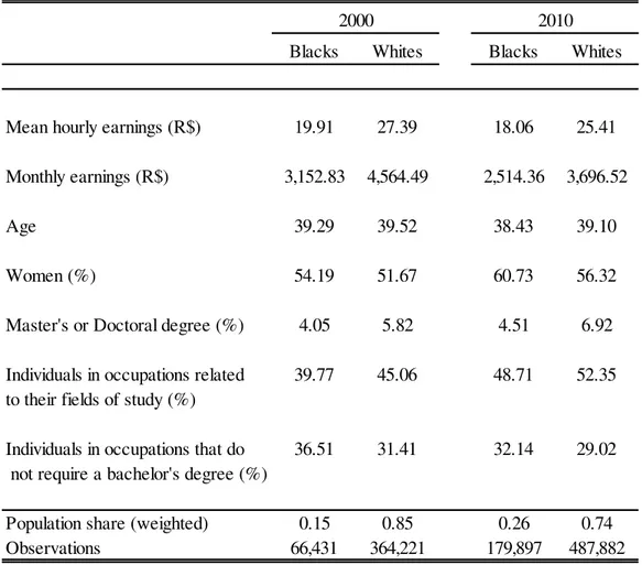
Table 2 reports the summary statistics regarding labor earnings, demographic

characteristics and education separately for white and black workers with at least a

bachelor’s degree in 2000 and 2010. It is possible to notice that black individuals

represented only 15% of the workers with tertiary education in Brazil in 2000, but 10

years later, the share of this group increased to one quarter. Table 2 shows that mean

hourly earnings among white workers with at least a bachelor’s degree (R$ 27.4) was

38% higher than that of black workers (R$ 19.9) with the same educational level in

2000, and that this differential increased to 41% in 2010. Comparing mean monthly

labor earnings, an even higher differential can be noticed between these two racial

groups, amounting to 45% in 2000 and to 47% in 2010.

As also shown in Table 2, black workers are slightly younger than white ones

and this age differential increased between 2000 and 2010. Women’s participation

among black workers with tertiary education was 54% in 2000, and augmented to 61%

10 years later. Among white workers with this level of education, the share of women

increased from 52% to 56% between 2000 and 2010.

The attainment of a graduate degree is much more common among white

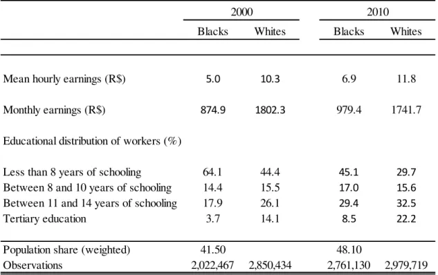
individuals than among black ones, which may help to explain part of the racial Table 1: Differences in labor earnings and education by race

Blacks Whites Blacks Whites

Mean hourly earnings (R$) 5.0 10.3 6.9 11.8

Monthly earnings (R$) 874.9 1802.3 979.4 1741.7

Educational distribution of workers (%)

Less than 8 years of schooling 64.1 44.4 45.1 29.7

Between 8 and 10 years of schooling 14.4 15.5 17.0 15.6

Between 11 and 14 years of schooling 17.9 26.1 29.4 32.5

Tertiary education 3.7 14.1 8.5 22.2

Population share (weighted) 41.50 48.10

Observations 2,022,467 2,850,434 2,761,130 2,979,719

Source: the 2000 and 2010 Brazilian Census.

Note: The sample includes occupied individuals, aged 25-60 years.

(9)

7

earnings gap, since workers with this level of education earn almost two times more

than those with just a bachelor’s degree, on average. Table 2 shows that 4.1% of the

black workers in the sample had a master’s or doctoral degree in 2000, and this

percentage improved only 0.4 percentage point in 10 years. Among white individuals,

5.8% had a master’s or doctoral degree in 2000, and this percentage increased to 6.9%

in 2010.

Forty percent of the black individuals were in occupations associated with their

fields of study in 2000, while among whites 45% were in this same situation. Between

2000 and 2010, the percentage of those in occupations considered related to the area of

study improved 9 percentage points among black individuals and 7 percentage points

among white ones. As also shown in Table 2, 36.5% of the black individuals in 2000

were working in occupations that require a lower level of education than a bachelor’s

Table 2: Descriptive statistics (workers with tertiary education).

Blacks Whites Blacks Whites

Mean hourly earnings (R$) 19.91 27.39 18.06 25.41

Monthly earnings (R$) 3,152.83 4,564.49 2,514.36 3,696.52

Age 39.29 39.52 38.43 39.10

Women (%) 54.19 51.67 60.73 56.32

Master's or Doctoral degree (%) 4.05 5.82 4.51 6.92

Individuals in occupations related 39.77 45.06 48.71 52.35 to their fields of study (%)

Individuals in occupations that do 36.51 31.41 32.14 29.02

not require a bachelor's degree (%)

Population share (weighted) 0.15 0.85 0.26 0.74

Observations 66,431 364,221 179,897 487,882

Note: The sample includes individuals with at least a bachelor's degree, aged 25-60 years, who are occupied.

(10)

8

degree, which was 5 percentage points higher compared to white individuals in the

same situation. This difference diminished 2 percentage points from 2000 to 2010.

Some human capital accumulated during tertiary education is occupation-specific, and

an individual may have an income penalty when his or her occupation does not match

the field of study (Robst, 2007; and Nordin et al., 2010) or requires a lower level of

schooling (Hartog, 2000). Thus, the descriptive statistics in Table 2 also suggest that

part of the earnings gap by race may be due to a job-education mismatch.

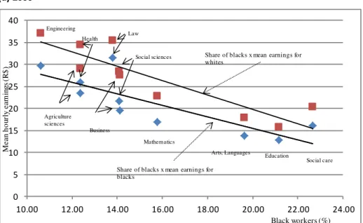
Figure 1: Share of black workers and mean hourly earnings by field of study

(a) 2000

(a) 2010

Note: The sample includes individuals with at least a bachelor's degree, aged 25-60 years, who are occupied. 0 5 10 15 20 25 30 35 40

10.00 12.00 14.00 16.00 18.00 20.00 22.00 24.00

M ea n h o ur ly e ar n in gs ( R $ )

Black workers (%)

Education Arts, Languages Mathematics Business Social sciences Law Agriculture sciences Engineering Health

Share of blacks x mean earnings for whites

Share of blacks x mean earnings for blacks 0 5 10 15 20 25 30 35 40

15.00 20.00 25.00 30.00 35.00 40.00

M ea n h o ur ly e ar n in gs ( R $ )

Black workers (%)

Education Social care Arts, Languages Mathem atics Business Social sciences Health Law Agriculture sciences Engineering

Share of blacks x mean earnings for whites

Share of blacks x mean earnings for blacks

(11)

9

Figure 1 presents the relationship between the participation of black workers in a

given field of study and the mean hourly labor earnings for white and black workers in

the same field. As can be seen, both periods reveal that the distribution of white and

black workers is very different across fields of study. In 2000, the share of black

individuals in each area of study ranges from 10.6% in engineering to 23% in social

care. The three fields with higher proportions of black individuals (education and arts,

languages and humanities, in addition to social care) are also those with lower mean

hourly earnings among black and white individuals in 2000, whereas fields with lower

percentages of blacks, such as engineering and health professions, have mean earnings

more than two times higher than the former ones.

Between 2000 and 2010, the share of black individuals improved in all fields of

study. In spite of this change, black workers in 2010 remained more concentrated in the

same areas as 10 years before. In fact, the most remarkable changes in terms of

percentage points occurred in fields with higher participation of black individuals in

2000. Another similarity between 2000 and 2010 data is the negative relationship

between the proportion of black workers and mean hourly earnings. In 2010, black

workers represented 38% of those who completed a program in education, but only 19%

of those who completed a program in engineering. Mean hourly earnings were R$ 12.4

for the former group and R$ 29.8 for the latter.

In summary, the racial earnings gap is very high in Brazil even among workers

with tertiary education, and the descriptive statistics suggest that a number of factors

could be associated with this differential. For example, the proportion of workers with a

graduate degree is lower among black than among white individuals, and the incidence

of mismatch between field of study and occupation is greater for black workers, who are

also more concentrated in fields of study that usually have lower labor earnings. The

next section presents the methods used in this paper for decomposing the relative

importance of each one of these factors on the earnings differential by race in 2000 and

(12)

10

4 – Decomposing the earnings gap by race

4.1 – Oaxaca-Blinder decomposition

The Oaxaca-Blinder methodology (Oaxaca, 1973 and Blinder, 1973) offers a

way to decompose differences in mean earnings between whites and blacks into

characteristic and price components. Following this method, suppose that the log hourly

labor earnings for individual i in racial group r (wir) can be written as:

(1) w_ir  X_ir_r e_ir_,

where Xir is a vector of characteristics (age, age squared, gender, state dummies, dummy

variables for residence in metropolitan and urban areas, a dummy for those who

concluded a master’s or doctoral degree, dummies for field of study, an indicator for

mismatch between area of study and occupation, and a dummy indicating that the

occupation does not require a bachelor’s degree). The term represents unobserved

factors, where it is assumed thatE



e_ir /X_ir



0, and _r is a vector of parameters. Thus, differences in mean earnings between whites (W) and blacks (B) can be

decomposed into two components:

(2) wW wB 



XW XB



ˆW 



ˆW ˆB



XB

The first term on the right side of equation (2) is the amount of the earnings gap

due to differences in characteristics, while the second term represents differences in the

returns on similar characteristics between white and black workers. Although the

Oaxaca-Blinder method offers a simple way to decompose earnings differences between

two groups, it has important limitations (Fortin, Lemieux and Firpo, 2011). It should be

mentioned, for example, that general equilibrium effects are not taken into account and

the results depend on the order of the decomposition. Also, Oaxaca-Blinder method is

useful only for decomposing mean differences. About this last point, decompositions for

different quantiles of the earnings distribution are performed using the method

(13)

11 4.2 –RIF-regression decomposition.

This subsection presents a brief description of the RIF-regression decomposition

method, following Fortin, Lemieux and Firpo (2009). This methodology allows

performing an Oaxaca-Blinder-type decomposition for different quantiles of the

earnings distribution. Thus, it is possible to investigate, for example, the role of

differences in the distribution of white and black workers across fields of study in the

earnings gap at the bottom as well as at the top of the earnings distribution.

A RIF-regression consists in estimating a regression similar to a standard one,

where the dependent variable is replaced with the recentered influence function (RIF)

for a quantile Q or another statistic of interest (Firpo, Fortin and Lemieux, 2009). The

influence function for a quantile Q is defined as:

(3) ( ) - ( )

( ) ,

where is the density of the marginal distribution of Y, and I(.) is an indicator

function. Thus, the ( ), which is equal to ( ), can be represented

by:

(4) ( ) ( )

( ) ( )

where

( ) and ( ) are constants. Thus, the RIF for a

quantile Q is a function of the constants c1,and c2,and a variable ( )

indicating whether labor earnings are smaller than or equal to the quantile QUsing

equation (4) and computing the estimates ̂ and ̂ ( ̂ ), it is possible to obtain an

estimate of the RIF:



(5) ̂ ( ) ̂ ( ̂ )

̂ ( ̂ )

Assuming that the conditional expectation of the RIF is a linear function of the

(14)

12

estimated by ordinary least squares. The coefficients of the unconditional quantile

regression () for a given racial group r in each quantile  can be estimated as follows:

(6) ̂ (∑ ) (∑ ̂ ( ) ).

Making use of the estimated coefficients in equation (6), it is possible to

compute a decomposition of the labor earnings gap by race for any quantile:

(7) ̂ ( ̅ ̅ ) ̂ ̅ ( ̂ ̂) ,

where the first term represents the characteristic effects, while the second term

represents the price differences. The former component can be represented as the sum of

the contributions of each covariate k:

(8) ̂ ∑( ̅ ̅) ̂

Then, it is possible to compute the contribution of differences between whites

and blacks regarding demographic characteristics, attainment of a graduate degree,

education-job mismatch and distribution across fields of study towards the earnings

differential between these two racial groups for each quantile of the earnings

distribution.

5 – Results

5.1 – Evidence for Oaxaca-Blinder decomposition

Table 3 presents the results for decompositions of the mean log hourly labor

earnings difference between white and black workers in 2000 into components due to

characteristic and price effects. The estimated contribution of each variable or set of

(15)

13

brackets in Table 3 display the share of the total difference between whites and blacks

attributed to each factor5.

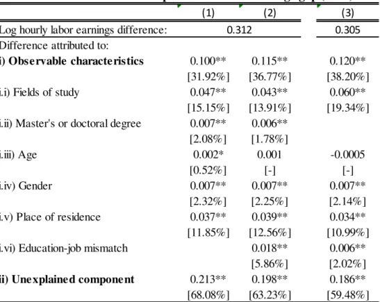
According to column (1), almost one third of the earnings difference by race in

2000 seems to be due to disparities in observed characteristics between white and black

workers. The estimated contribution of differences in fields of study corresponds to

15% of the total gap, which is half of the difference associated with characteristics.

Regional distribution of white and black workers represents 12% of the earnings gap

between these two groups, while differences regarding the attainment of a graduate

degree, and composition by age and gender seem to play a minor or non-significant

role.

5

Table B.1 in the appendix reports the estimated coefficients of selected variables in log labor earnings regressions for white and black individuals in 2000 and 2010.

Table 3: Oaxaca-Blinder decomposition of racial earnings gap (2000)

(1) (2) (3)

Log hourly labor earnings difference: 0.305

Difference attributed to:

i) Observable characteristics 0.100** 0.115** 0.120**

[31.92%] [36.77%] [38.20%]

i.i) Fields of study 0.047** 0.043** 0.060**

[15.15%] [13.91%] [19.34%]

i.ii) Master's or doctoral degree 0.007** 0.006** [2.08%] [1.78%]

i.iii) Age 0.002* 0.001 -0.0005

[0.52%] [-] [-]

i.iv) Gender 0.007** 0.007** 0.007**

[2.32%] [2.25%] [2.14%]

i.v) Place of residence 0.037** 0.039** 0.034**

[11.85%] [12.56%] [10.99%]

i.vi) Education-job mismatch 0.018** 0.006**

[5.86%] [2.02%]

ii) Unexplained component 0.213** 0.198** 0.186**

[68.08%] [63.23%] [59.48%]

Source: the 2000 Brazilian Census.

Note: place of residence is represented by 26 state dummies, and dummy variables for metropolitan and urban areas. Education-job mismatch is represented by a dummy for individuals in occupations unrelated to their degrees and a dummy for those in

occupations that do not require a bachelor's degree. In columns (1) and (2), fields of study are represented by 10 groups, while column (3) considers 35 groups. Decomposition in column (3) excludes individuals with a graduate degree. Values in brackets show the share of the total difference attributed to each factor.

(16)

14

Decomposition in column (2) considers the contribution of variables

representing the mismatch between education and job. In this case, the share of the

earnings differential due to characteristics increases from 32% to 37%. The estimated

contributions of the terms reported in column (1) remain almost the same, including the

one representing differences in field of study composition by race. Around 4% of the

earnings difference between white and black workers is associated with education-job

mismatch, according to estimates.

The results in column (3) are estimated using a more disaggregated classification

with 35 fields of study. Because graduate degree is defined only for 9 aggregated areas

in 2000 and fields of study refer to the individuals’ highest degree, decomposition in

column (3) is limited to those who have only a bachelor’s degree. Individuals who

concluded a program in one of the six fields in 2000 for whom a corresponding one in

2010 is not assigned, as shown in the appendix, are also excluded. Column (3) indicates

that differences in the characteristics of white and black workers represent 38% of the

earnings gap by race. About half of this differential is attributed to the distribution of

each racial group across fields of study.

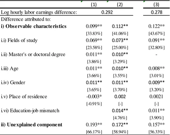
Table 4 reports the estimated results for 2010. As can be seen in column (1), the

characteristic effects represent 34% of the difference in mean hourly labor earnings

between whites and blacks. Differences in racial composition across fields of study

contribute to one quarter of the total difference in mean earnings, which represents 70%

of the share associated with the characteristic effects.

In column (2), the inclusion of education-job mismatch variables increases the

contribution of the characteristic effects from 34% to 41%. Indeed, most of this change

is related to effects associated with education-job mismatch. According to estimates in

column (3), using a classification of areas of study with 35 categories, as in column (3)

of Table 3, the characteristic effects represent 44% of the mean earnings differential

between white and black workers in 2010. Most of this component seems to be due to

differences in field of study composition by race, which contributes with one third of

the total difference, and with 75% of the share associated with the characteristic effects.

The estimated effects associated with differences in the other covariates are similar to

those reported in the first two columns of Table 4.

According to estimates, the share of racial earnings difference attributed to

disparities in the distribution of whites and blacks across fields of study is larger in 2010

(17)

15

differential in both years, disparities in fields of study composition account for half of

this component in 2000, and 70% in 2010. In the former period, regional distribution

contributes with 12% of the total racial earnings gap, but the effect associated with this

term is close to zero in 2010. Comparisons between Tables 3 and 4 should be made with

caution because the classification system is not the same in the 2000 and 2010 Census,

as described in the appendix. Nevertheless, this evidence is also verified for a number of

different classifications of fields of study adopted.6

6

In addition, decompositions of the racial hourly earnings gap in 2010 using the aggregated classification provided by the 2010 Census with 8 groups, instead of the one adopted in the estimates reported in Table 4, show that differences regarding fields of study contribute with 23% of the total gap. This value is very similar to the estimated effects in columns (1) and (2) of Table 4.

Table 4: Oaxaca-Blinder decomposition of racial earnings gap (2010)

(1) (2) (3)

Log hourly labor earnings difference: 0.278

i) Observable characteristics 0.099** 0.112** 0.122**

[33.83%] [41.06%] [43.67%]

i.i) Fields of study 0.069** 0.073** 0.091**

[23.58%] [25.00%] [32.80%]

i.ii) Master's or doctoral degree 0.011** 0.010**

-[3.86%] [3.29%]

i.iii) Age 0.011** 0.010** 0.008**

[3.66%] [3.55%] [3.01%]

i.iv) Gender 0.011** 0.011** 0.009**

[3.65%] [3.70%] [3.20%]

i.v) Place of residence -0.003* 0.002 0.0021

[-0.91%] [-] [-]

i.vi) Education-job mismatch 0.014** 0.011**

[4.76%] [3.90%]

ii) Unexplained component 0.193** 0.172** 0.157**

[66.17%] [58.94%] [56.33%]

Note: place of residence is represented by 26 state dummies, and dummy variables for metropolitan and urban areas. Education-job mismatch is represented by a dummy for individuals in occupations unrelated to their degrees and a dummy for those in

occupations that do not require a bachelor's degree. In columns (1) and (2), fields of study are represented by 10 groups, while column (3) considers 35 groups. Decomposition in column (3) excludes individuals with a graduate degree. Values in brackets show the share of the total difference attributed to each factor.

(18)

16

The results presented in this subsection are robust to other specifications, which

include changing the order of the decomposition in equation (2) and using monthly

instead of hourly earnings. In another robustness check, the analysis is carried out

separately by gender, without changes in the main conclusions about the role of

disparities in field of study composition in earnings differential by race.7

Decompositions are also performed using the Juhn, Murphy and Pierce (1993) method,

and the results, reported in appendix C, are very similar to those presented in Tables 3

and 4.

5.2 – Evidence for RIF-regression decomposition

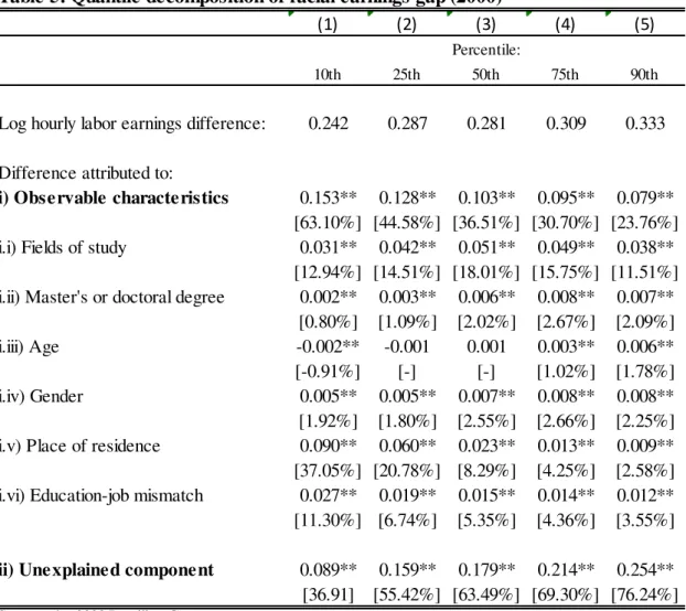
Table 5 reports racial earnings gap decomposition of the 10th, 25th, 50th, 75th, and

90th percentiles of the unconditioned distribution of hourly labor earnings for 2000.8 It

can be noticed that the earnings differential is much larger at the top of the distribution

than at the bottom. Also, the share of the racial difference attributed to individuals’

characteristics seems to be more important at lower percentiles of the distribution. At

the 10th percentile, differences in observable characteristics of white and black workers

represent almost two thirds of the hourly earnings gap between these two groups, while

this component represents only one quarter of the racial earnings gap at the 90th

percentile.

Estimates indicate that the distribution of whites and blacks across areas of study

accounts for 18% of the total difference in hourly earnings by race at the median of the

distribution. At the 10th and 90th percentiles, the estimated contributions of this factor

represent 13% and 12% of the total. About the other characteristic effects, racial

differences in regional distribution and education-job mismatch, in particular the

proportion of workers with at least a bachelor’s degree who work in occupations that do

not require this level of education, seem to represent an important share of the earnings

gap by race at the 10th percentile, but the effects associated with these factors become

less important at the top of the distribution.

7

These results are available upon request.

8

(19)

17

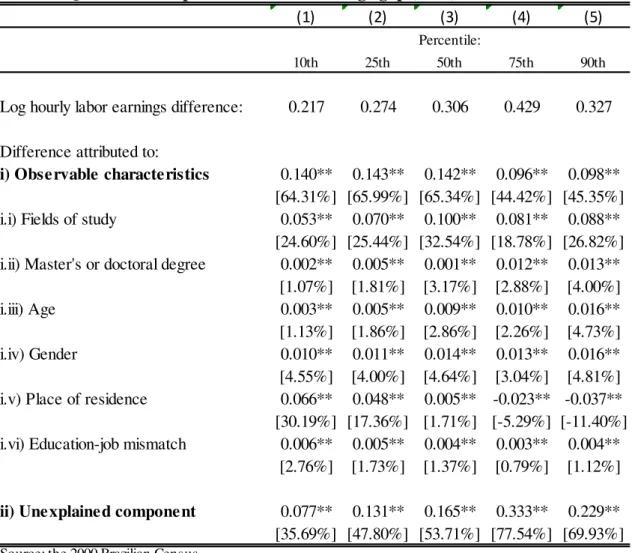
Table 6 reports the results of quantile decompositions of the earnings

distribution in 2010. Hourly earnings differential between white and black workers is

also higher at the top of the distribution, while the contribution of characteristic effects

is higher at the lower part of the distribution. These patterns are similar to the ones

reported in Table 5 for 2000. Disparities in the distribution of whites and blacks across

fields of study represent about one quarter of the earnings gap by race at the 10th, 25th

and 90th percentiles, and 19% at the 75th percentile.

The relative importance of differences in fields of study reaches its highest value

at the 50th percentile, corresponding to 33% of the total difference. Therefore,

decompositions using RIF-regressions also suggest that the share of the earnings

differential by race attributed to disparities in the distributions of whites and blacks

Table 5: Quantile decomposition of racial earnings gap (2000)

(1) (2) (3) (4) (5)

10th 25th 50th 75th 90th

Log hourly labor earnings difference: 0.242 0.287 0.281 0.309 0.333

i) Observable characteristics 0.153** 0.128** 0.103** 0.095** 0.079** [63.10%] [44.58%] [36.51%] [30.70%] [23.76%]

i.i) Fields of study 0.031** 0.042** 0.051** 0.049** 0.038**

[12.94%] [14.51%] [18.01%] [15.75%] [11.51%] i.ii) Master's or doctoral degree 0.002** 0.003** 0.006** 0.008** 0.007**

[0.80%] [1.09%] [2.02%] [2.67%] [2.09%]

i.iii) Age -0.002** -0.001 0.001 0.003** 0.006**

[-0.91%] [-] [-] [1.02%] [1.78%]

i.iv) Gender 0.005** 0.005** 0.007** 0.008** 0.008**

[1.92%] [1.80%] [2.55%] [2.66%] [2.25%]

i.v) Place of residence 0.090** 0.060** 0.023** 0.013** 0.009**

[37.05%] [20.78%] [8.29%] [4.25%] [2.58%] i.vi) Education-job mismatch 0.027** 0.019** 0.015** 0.014** 0.012** [11.30%] [6.74%] [5.35%] [4.36%] [3.55%]

ii) Unexplained component 0.089** 0.159** 0.179** 0.214** 0.254** [36.91] [55.42%] [63.49%] [69.30%] [76.24%]

Note: place of residence is represented by 26 state dummies, and dummy variables for metropolitan and urban areas. Education-job mismatch is represented by a dummy for individuals in occupations unrelated to their degrees and a dummy for those in occupations that do not require a bachelor's degree. Values in brackets show the share of the total difference attributed to each factor.

* significant at the level of 5%, ** significant at the level of 1%.

(20)

18

across fields of study is larger for 2010 compared to 2000. At the top half of the

earnings distribution in 2010, it can be noticed that almost all of the racial earnings gap

due to characteristic effects is represented by differences in field of study composition.

In 2000, the contribution of this term at the 75th and 90th percentiles corresponded to

half of the estimated characteristic effects.

Also according to Table 6, regional composition by race represents an important

share of the earnings gap at the bottom of the distribution, whereas differences

regarding age and the attainment of a master’s or doctoral degree are more important at

the top of the distribution than at lower percentiles.

Table 6: Quantile decomposition of racial earnings gap (2010)

(1) (2) (3) (4) (5)

10th 25th 50th 75th 90th

Log hourly labor earnings difference: 0.217 0.274 0.306 0.429 0.327

i) Observable characteristics 0.140** 0.143** 0.142** 0.096** 0.098** [64.31%] [65.99%] [65.34%] [44.42%] [45.35%]

i.i) Fields of study 0.053** 0.070** 0.100** 0.081** 0.088**

[24.60%] [25.44%] [32.54%] [18.78%] [26.82%] i.ii) Master's or doctoral degree 0.002** 0.005** 0.001** 0.012** 0.013**

[1.07%] [1.81%] [3.17%] [2.88%] [4.00%]

i.iii) Age 0.003** 0.005** 0.009** 0.010** 0.016**

[1.13%] [1.86%] [2.86%] [2.26%] [4.73%]

i.iv) Gender 0.010** 0.011** 0.014** 0.013** 0.016**

[4.55%] [4.00%] [4.64%] [3.04%] [4.81%]

i.v) Place of residence 0.066** 0.048** 0.005** -0.023** -0.037**

[30.19%] [17.36%] [1.71%] [-5.29%] [-11.40%] i.vi) Education-job mismatch 0.006** 0.005** 0.004** 0.003** 0.004**

[2.76%] [1.73%] [1.37%] [0.79%] [1.12%]

ii) Unexplained component 0.077** 0.131** 0.165** 0.333** 0.229** [35.69%] [47.80%] [53.71%] [77.54%] [69.93%]

Note: place of residence is represented by 26 state dummies, and dummy variables for metropolitan and urban areas. Education-job mismatch is represented by a dummy for individuals in occupations

unrelated to their degrees and a dummy for those in occupations that do not require a bachelor's degree. Values in brackets show the share of the total difference attributed to each factor.

(21)

19

6 - Conclusions

The labor earnings differential between white and black workers is very high in

Brazil, even restricting the comparison to individuals who completed at least a

bachelor’s degree. This paper analyzes whether racial differences in the distribution of

workers across fields of study contribute to this earnings gap, using Brazilian Census

data from 2000 and 2010.

Estimates indicate that 14% of the difference in mean earnings by race in 2000

seems to be due to the fact that black individuals were much more concentrated in fields

of study with lower mean earnings. Between 2000 and 2010, the percentage of black

workers who completed at least a bachelor’s degree increased from 3.7% to 8.5%,

which is still much lower compared to whites with this same educational level (22.2%).

In addition, 10 years later, black individuals remained concentrated in fields of study

where labor earnings are usually lower. In 2010, racial disparities in fields of study

composition represent 25% of the mean earnings gap, according to estimates.

Evidence also shows that earnings difference by race is greater at the top of the

distribution than at the bottom. Quantile decompositions of the earnings distribution

indicate that field of study composition by race seems to be more important in

explaining total earnings difference at the median of the distribution, representing 18%

of the gap in 2000 and 33% in 2010.

Thus, the results suggest that black individuals are underrepresented not only in

the group of workers with a bachelor’s or graduate degree, but also in fields of study

where labor earnings are usually higher, which helps to explain part of the elevated

earnings differential by race among highly educated individuals in Brazil. Also, it seems

that the improvement over time in the proportion of black workers with tertiary

education has been mainly driven by fields with low mean earnings, contributing to

(22)

20

References:

Altonji, J. G. (1993). The demand for and return to education when education outcomes

are uncertain. Journal of Labour Economics, 11(1),48–83.

Blinder, A. (1973). Wage discrimination: Reduced form and structural estimates.

Journal of Human Resources 8 (4), 436-855.

Blundell, R., Dearden, L., Goodman, A., & Reed, H. (2000). The returns to higher

education in Britain: Evidence from a British cohort. The Economic Journal, 110(461),

F82–F99.

Classificação Brasileira de Ocupações, 2010. Ministério do Trabalho e do Emprego,

Brasília, 3ª. edição.

Finnie, R., & Frenette, M. (2003). Earnings differences by major field of study:

Evidence from three cohorts of recent Canadian graduates. Economics of Education

Review, 22(2), 179–192.

Firpo, S., Fortin, N. and T. Lemieux, 2009. “Unconditional Quantile Regressions”,

Econometrica, 77(3), pp. 953-973.

Fortin, N., Lemieux, T. and S. Firpo, S., 2011. Decomposition Methods in Economics,

Handbook of Labor Economics, Vol. 4A, Pages 1-102.

Hartog, J. (2000). “Overeducation and earnings. Where are we, where should we go?”

Economics of Education Review, 19(2), 131–147.

Juhn, C., Murphy, K., Pierce, B., 1993. Wage inequality and the rise in returns to skill.

Journal of Political Economy 101 (3), 410-442.

Nordin, M., Persson, I. and R. Dan-Olof, 2010. “Education–occupation mismatch: Is

(23)

21

Oaxaca, R. L. “Male-female wage differentials in urban labor markets”, International Economic Review, 14, 1973, p. 693-709.

Robst, J. (2007a). “Education and job match: The relatedness of college major and

(24)

22

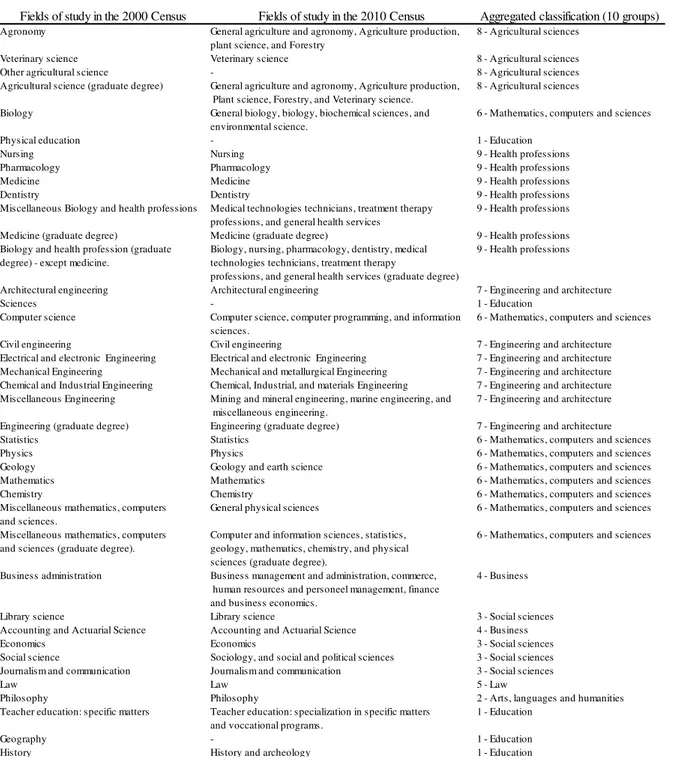
Appendix A

The 2000 Brazilian Census classifies individuals with a bachelor’s degree into

41 fields of study, and those with a graduate degree (master’s or doctoral, without

distinction between them) into 9 groups. In the 2010 Census, individuals with a

bachelor’s degree are classified into 89 areas of study, which are similar to the ones

available to classify those with a master’s or doctoral degree. In both periods, an

individual’s field of study is defined according to his or her highest educational degree.

The 2000 and 2010 codes for field of study are matched following the

description reported in Table A1 (columns (1) and (2)). For many areas of study, mainly

for those comprising an important share of the individuals with tertiary education in

Brazil, such as medicine and law, the match is clear. As can be seen, there are fields in

the 2000 classification system, such as business administration and arts, which refer to

many narrower codes in the 2010 system. Also, a few codes in 2000 are not assigned to

a code in 2010. This is done in situations where the program in the former system does

not have an equivalent one in the latter (geography, physical education), or the match is

not considered clear, as are the cases of science programs, other agriculture programs,

other social science, and other arts and languages programs.

The 41 fields of study are aggregated into 10 groups, as reported in column (3)

of Table A1, which may help to mitigate part of the problems due to missing or unclear

correspondence. It can be noticed that a few programs related to sciences and social

sciences are classified as education in the aggregated classification. This is done

because comparisons between data from 2000 and 2010 show a remarkable reduction in

the participation of these groups over time, which could be due to the fact that the 2010

system has a more detailed classification for programs in education. The estimated

results are robust to other criteria used to classify these areas of study.

It should be also mentioned that the 2000 census classification system

aggregates the 41 groups defined for those with a bachelor’s degree into 9 graduate

categories. This restriction causes a problem when a graduate group includes programs

assigned to different areas in the aggregated classification, as is the case, for example,

(25)

23

Table A.1: Fields of study in the 2000 and 2010 Brazilian census

Fields of study in the 2000 Census Fields of study in the 2010 Census Aggregated classification (10 groups) Agronomy General agriculture and agronomy, Agriculture production, 8 - Agricultural sciences

plant science, and Forestry

Veterinary science Veterinary science 8 - Agricultural sciences Other agricultural science - 8 - Agricultural sciences Agricultural science (graduate degree) General agriculture and agronomy, Agriculture production, 8 - Agricultural sciences

Plant science, Forestry, and Veterinary science.

Biology General biology, biology, biochemical sciences, and 6 - Mathematics, computers and sciences environmental science.

Physical education - 1 - Education

Nursing Nursing 9 - Health professions

Pharmacology Pharmacology 9 - Health professions

Medicine Medicine 9 - Health professions

Dentistry Dentistry 9 - Health professions Miscellaneous Biology and health professions Medical technologies technicians, treatment therapy 9 - Health professions

professions, and general health services

Medicine (graduate degree) Medicine (graduate degree) 9 - Health professions Biology and health profession (graduate Biology, nursing, pharmacology, dentistry, medical 9 - Health professions degree) - except medicine. technologies technicians, treatment therapy

professions, and general health services (graduate degree)

Architectural engineering Architectural engineering 7 - Engineering and architecture

Sciences - 1 - Education

Computer science Computer science, computer programming, and information 6 - Mathematics, computers and sciences sciences.

Civil engineering Civil engineering 7 - Engineering and architecture Electrical and electronic Engineering Electrical and electronic Engineering 7 - Engineering and architecture Mechanical Engineering Mechanical and metallurgical Engineering 7 - Engineering and architecture Chemical and Industrial Engineering Chemical, Industrial, and materials Engineering 7 - Engineering and architecture Miscellaneous Engineering Mining and mineral engineering, marine engineering, and 7 - Engineering and architecture

miscellaneous engineering.

Engineering (graduate degree) Engineering (graduate degree) 7 - Engineering and architecture Statistics Statistics 6 - Mathematics, computers and sciences Physics Physics 6 - Mathematics, computers and sciences Geology Geology and earth science 6 - Mathematics, computers and sciences Mathematics Mathematics 6 - Mathematics, computers and sciences Chemistry Chemistry 6 - Mathematics, computers and sciences Miscellaneous mathematics, computers General physical sciences 6 - Mathematics, computers and sciences and sciences.

Miscellaneous mathematics, computers Computer and information sciences, statistics, 6 - Mathematics, computers and sciences and sciences (graduate degree). geology, mathematics, chemistry, and physical

sciences (graduate degree).

Business administration Business management and administration, commerce, 4 - Business human resources and personeel management, finance

and business economics.

Library science Library science 3 - Social sciences Accounting and Actuarial Science Accounting and Actuarial Science 4 - Business

Economics Economics 3 - Social sciences

Social science Sociology, and social and political sciences 3 - Social sciences Journalism and communication Journalism and communication 3 - Social sciences

Law Law 5 - Law

Philosophy Philosophy 2 - Arts, languages and humanities Teacher education: specific matters Teacher education: specialization in specific matters 1 - Education

and voccational programs.

Geography - 1 - Education

(26)

24

Table A.1 (continued)

Fields of study in the 2000 Census Fields of study in the 2010 Census Aggregated classification (10 groups) Teacher education Elementary, secondary and early childhood 1 - Education

education, miscellaneous education.

Advertising and marketing Advertising and marketing 4 - Business Psychology Psychology 3 - Social sciences Social work Social work 10 - Social care

Theology Theology 2 - Arts, languages and humanities Miscellaneous Social Sciences and humanities - 3 - Social sciences

Business administration (graduate degree) Business management and administration, and 4 - Business advertising and marketing (graduate degree).

Economics and accounting (graduate degree) Economics and accounting (graduate degree) 3 - Social sciences Law (graduate degree) Law (graduate degree) 5 - Law Teacher education (graduate degree) Elementary, secondary and early childhood 1 - Education

education, voccational programs teacher education, teacher with specialization in specific matters, and miscellaneous education (graduate degree).

Miscellaneous Social Sciences and humanities Psychology, Sociology, and social and political sciences, 3 - Social sciences (graduate degree). Journalism and communication (graduate degree).

Languages And Literature Foreign languagues, portuguese language, literature 2 - Arts, languages and humanities and miscellaneous languages and humanities.

Arts Fine arts, drama and theater arts, music, visual and 2 - Arts, languages and humanities performing arts, commercial art and graphic design.

Miscellaneous Arts, languages and literature - 2 - Arts, languages and humanities Miscellaneous Arts, languages and literature Foreign languagues, portuguese language, literature 2 - Arts, languages and humanities (graduate degree). and miscellaneous languages and humanities, fine arts,

(27)

25

Appendix B

Table B.1: Estimated coefficients of selected variables in log earnings regressions (OLS)

(1) (2) (3) (4)

Black White Black White

Fields of study Education (ref.)

Arts, languages and humanities 0.0614 0.0971 0.0892 0.1519

[5.60]** [18.22]** [10.60]** [25.82]**

Social sciences 0.2586 0.2996 0.3371 0.3711

[22.00]** [57.82]** [29.97]** [60.92]**

Business 0.2332 0.2491 0.2683 0.3444

[22.53]** [53.66]** [38.45]** [81.63]**

Law 0.5396 0.4646 0.5874 0.5474

[42.09]** [85.93]** [56.14]** [100.78]**

Mathematics, computers ans sciences 0.2011 0.2237 0.2436 0.2838

[16.81]** [41.82]** [28.58]** [54.22]**

Engineering and architecture 0.4713 0.4752 0.5615 0.5901

[32.99]** [88.02]** [50.58]** [105.37]**

Agricultural sciences 0.3412 0.3302 0.3687 0.4462

[14.03]** [36.86]** [21.09]** [49.02]**

Health professions 0.4758 0.5159 0.4131 0.4777

[41.57]** [109.87]** [52.18]** [107.16]**

Social care 0.1928 0.1597 0.275 0.2673

[10.26]** [15.43]** [16.11]** [22.37]**

Master's or doctoral degree 0.3311 0.3135 0.3991 0.4041

[20.25]** [56.01]** [34.54]** [73.76]**

Age 0.082 0.0824 0.0474 0.0687

[25.45]** [61.84]** [22.16]** [54.11]**

Age squared -0.0008 -0.0008 -0.0003 -0.0006

[19.55]** [46.08]** [13.03]** [37.32]**

Female -0.2075 -0.2785 -0.2523 -0.2553

[30.85]** [94.63]** [52.39]** [87.15]**

Occupation related to the field of study 0.1148 0.1226 0.1195 0.1459 [13.35]** [34.34]** [17.81]** [37.98]**

Occupation that does not require -0.2544 -0.2316 -0.3073 -0.2742

tertiary education [30.26]** [62.88]** [45.21]** [66.92]**

Constant 0.6768 0.7916 0.9792 0.607

[8.86]** [21.06]** [21.28]** [19.57]**

R-squared 0.24 0.27 0.25 0.26

Observations 66,431 364,221 182,905 496,201

Note: Regressions also include 26 state dummies, and dummy variables for metropolitan and urban areas. t-statistics are in brackets.

(28)

26

Table B.2: RIF-regression results (2000)

(1) (2) (3) (4) (5) (6)

Percentile: 10th 50th 90th 10th 50th 90th

Arts, languages and humanities -0.0046 0.0832 0.1197 0.0444 0.1225 0.0790

[0.20] [5.58]** [6.19]** [3.26]** [18.75]** [11.40]**

Social sciences 0.1240 0.3008 0.3497 0.1809 0.3638 0.2592

[5.90]** [20.02]** [13.58]** [15.55]** [57.77]** [30.11]**

Business 0.0792 0.2927 0.3455 0.1090 0.3187 0.2049

[4.03]** [22.18]** [16.22]** [9.82]** [56.46]** [29.16]**

Law 0.2467 0.5321 0.9922 0.2932 0.5069 0.5204

[13.84]** [35.44]** [29.28]** [26.84]** [79.63]** [52.30]**

Mathematics, computers ans sciences 0.1750 0.2497 0.2003 0.2384 0.2610 0.1106

[7.79]** [15.41]** [8.02]** [19.03]** [37.86]** [13.40]**

Engineering and architecture 0.2115 0.5361 0.7010 0.3292 0.5671 0.3996

[9.99]** [31.27]** [18.42]** [30.88]** [86.34]** [37.54]**

Agricultural sciences 0.2641 0.4094 0.3869 0.3289 0.4074 0.1300

[7.59]** [14.24]** [6.45]** [18.80]** [37.66]** [8.48]**

Health professions 0.2206 0.5424 0.6801 0.3912 0.5978 0.4667

[12.53]** [37.07]** [23.20]** [40.13]** [101.34]** [52.66]**

Social care 0.0793 0.2317 0.1531 0.1160 0.2275 0.0264

[2.14]* [8.68]** [4.22]** [4.68]** [16.37]** [1.89]

Master's or doctoral degree 0.0762 0.2972 0.8097 0.1079 0.3369 0.4089

[4.13]** [16.65]** [15.26]** [14.33]** [55.50]** [28.35]**

Age 0.0983 0.0916 0.0545 0.1168 0.0939 0.0317

[17.00]** [23.42]** [7.33]** [42.38]** [61.44]** [12.71]**

Age squared -0.0010 -0.0009 -0.0004 -0.0013 -0.0009 -0.0001

[15.06]** [18.57]** [3.84]** [38.17]** [48.70]** [2.33]*

Female -0.0785 -0.2312 -0.3320 -0.1915 -0.2935 -0.3158

[6.95]** [27.22]** [21.41]** [32.61]** [82.81]** [58.82]**

Occupation related to the field of study 0.0589 0.1238 0.1570 0.1197 0.1205 0.1132

[4.65]** [11.32]** [7.26]** [18.58]** [28.03]** [16.09]**

Occupation that does not require -0.4435 -0.2158 -0.1339 -0.4324 -0.1927 -0.1427 tertiary education [29.76]** [20.04]** [7.29]** [54.33]** [43.77]** [23.21]**

Constant -0.5831 0.4953 2.1970 -0.7531 0.4753 2.9311

[4.18]** [5.29]** [12.74]** [9.61]** [10.7]** [44.34]**

R-squared

Observations 66,431 66,431 66,431 364,221 364,221 364,221

(29)

27

Table B.3: RIF-regression results (2010)

(1) (2) (3) (4) (5) (6)

Percentile: 10th 50th 90th 10th 50th 90th

Arts, languages and humanities 0.0606 0.1049 0.1344 0.1203 0.183 0.1442

[4.20]** [9.95]** [7.19]** [12.42]** [24.10]** [12.02]**

Social sciences 0.2101 0.3794 0.4843 0.269 0.4532 0.3764

[14.43]** [29.26]** [15.95]** [32.90]** [60.30]** [24.81]**

Business 0.1893 0.2702 0.398 0.2211 0.4133 0.3814

[16.44]** [31.75]** [24.22]** [32.09]** [76.66]** [41.47]**

Law 0.2579 0.5643 1.0637 0.3255 0.6107 0.7795

[22.01]** [53.06]** [36.65]** [47.06]** [97.58]** [56.72]**

Mathematics, computers ans sciences 0.1663 0.2787 0.333 0.2057 0.3686 0.2206

[12.87]** [26.72]** [15.16]** [25.59]** [54.10]** [18.04]**

Engineering and architecture 0.2433 0.5816 0.9036 0.338 0.7132 0.6658

[18.42]** [48.82]** [27.09]** [48.35]** [107.73]** [42.51]**

Agricultural sciences 0.1947 0.449 0.4826 0.3062 0.5757 0.3933

[8.19]** [22.41]** [9.88]** [25.48]** [53.39]** [17.65]**

Health professions 0.1781 0.4458 0.6753 0.286 0.5484 0.6097

[15.44]** [47.81]** [32.49]** [43.44]** [98.02]** [55.69]**

Social care 0.1056 0.3124 0.4158 0.2058 0.3338 0.1979

[3.98]** [15.09]** [9.81]** [11.41]** [20.63]** [7.65]**

Master's or doctoral degree 0.0459 0.3597 0.9695 0.0965 0.4088 0.6591

[4.13]** [32.18]** [24.66]** [19.98]** [71.60]** [35.13]**

Age 0.0628 0.0562 0.0262 0.073 0.0789 0.0416

[19.82]** [22.94]** [4.77]** [41.83]** [53.23]** [12.81]**

Age squared -0.0006 -0.0005 0.000 -0.0007 -0.0007 -0.0001

[16.52]** [15.13]** [0.55] [36.12]** [39.31]** [3.07]**

Female -0.1869 -0.2398 -0.3805 -0.1643 -0.2632 -0.3587

[27.03]** [42.36]** [30.73]** [42.69]** [74.75]** [48.04]**

Occupation related to the field of study 0.1093 0.1101 0.199 0.0841 0.1546 0.1985

[13.14]** [14.23]** [10.94]** [18.75]** [33.25]** [19.78]**

Occupation that does not require -0.5041 -0.2909 -0.1825 -0.4484 -0.2425 -0.1611 tertiary education [49.44]** [36.66]** [10.89]** [76.13]** [48.28]** [16.90]**

Constant 0.0432 0.5834 2.2874 -0.1956 0.1938 2.235

[0.61] [10.80]** [19.90]** [4.40]** [5.25]** [29.70]**

R-squared

Observations 182,905 182,905 182,905 496,201 496,201 496,201

(30)

28

Table C1: Juhn, Murphy and Pierce decomposition of racial earnings gap

Log hourly labor earnings difference:

(1) (2) (3) (4)

i) Observable characteristics 0.100 0.115 0.099 0.120

[31.87%] [36.73%] [33.81%] [41.03%]

i.i) Fields of study 0.047 0.043 0.069 0.073

[15.11%] [13.87%] [23.55%] [24.98%]

i.ii) Master's or doctoral degree 0.006 0.006 0.011 0.010

[2.08%] [1.78%] [3.86%] [3.29%]

i.iii) Age 0.002 0.001 0.011 0.010

[0.52%] [0.40%] [3.66%] [3.55%]

i.iv) Gender 0.007 0.007 0.011 0.011

[2.32%] [2.25%] [3.65%] [3.70%]

i.v) Place of residence 0.037 0.039 -0.003 0.002

[11.85%] [12.56%] [-0.91%] [0.75%]

i.vi) Education-job mismatch - 0.018 - 0.014

[5.86%] [4.76%]

ii) Observable prices 0.213 0.198 0.193 0.172

[68.08%] [63.23%] [66.17%] [58.94%]

iii) Unobservable prices 0.000 0.000 0.000 0.000

[0.04%] [0.04%] [0.02%] [0.02%]

Note: place of residence is represented by 26 state dummies, and dummy variables for metropolitan and urban areas. Education-job mismatch is represented by a dummy for individuals in occupations unrelated to their degrees and a dummy for those in occupations that do not require a bachelor's degree. Fields of study are represented by 10 groups. Values in brackets show the share of the total difference attributed to each factor.

2000 2010