Football players’ transfer price determination based on performance in the Big 5 European leagues

1

A Work Project, presented as part of the requirements for the Award of a Master Degree in

Economics from the NOVA – School of Business and Economics.

Football players’ transfer price determination based on

performance in the Big 5 European leagues

Jean-Sébastien Jacques Emile Marie Ghislain Geurts, 751

A Project carried out on the Master in Economics Program, under the supervision of:

Professor Paulo Manuel Marques Rodrigues

2

Abstract

The existing literature on the determinants of football players’ transfer prices considers bargaining theory and identifies buyer and seller characteristics as main influences. No

attention has been brought to performance measures which were directly observable and

quantifiable. This study uses a normalised position-specific performance measure to

investigate the issue. It finds evidence that player performance does play a role in the

determination of transfer prices although the model suffers from incoherencies. The model also

investigates a player’s previous contract duration’s effect on the amount of the transfer fee

paid. A positive relationship between months remaining on a player’s contract and the fee paid for that player has been found.

Acknowledgements:

I would like to thank my supervisor, Professor Rodrigues, for his guidance during the

elaboration of this research as well as my parents for their unconditional and unwavering

3

Table of contents

I. Introduction ... 4

II. Literature review ... 5

1. Club objectives... 5

2. Football labour market and regulations ... 7

3. Empirical evidence of the determinants of player transfer prices ... 8

III. The data ... 12

IV. The model ... 13

1. Player performance ... 13

2. Model specification ... 16

V. Results ... 17

1. Main findings ... 18

2. Robustness checks ... 19

3. Interpretation and limitations ... 20

VI. Conclusion ... 21

4

I.

Football is the world’s most popular sport. According to FIFA, football’s international

governing organization, 3.2 billion people watched the FIFA World Cup 2014 final from their

television at home. National football federations compete heavily on being awarded its

organization and are ready to do almost anything to do so as shown by recent corruption

scandals. Football is growing, clubs expand their fan base internationally and broadcasting

revenues increase every year. The major European leagues (French Ligue 1, English Premier

League, Spanish Liga, Italian Serie A and the German Bundesliga), referred to as the Big 5,

concentrate the financially most powerful football clubs on the planet. The total international

transfer expenditure in 2014 was estimated by FIFA at 3.6 billion USD which stresses the

economic importance of the football market.

Academic researchers began showing interest around 1970 with the first influential analysis of

the football industry made by Sloane (1969). With the growing media attention and the

extensive regulation of the football labour market Fricks (2007) observes that statistical data

on transfer and salaries has become readily available. Sports is considered a perfect

environment to test competition and labour market theories (Sloane, 2015). Hence, a large body

of the literature attempted to find the determinants of transfer prices and player salaries as well

as analysing the industry in terms of competitive balance.

This research will focus on transfers. Transfer expenditure per clubs, as measured as the

combined expenditure of all players who have been transferred to a club has been growing in

the big five over the last five years (Poli et al., 2015a). Although most studies use bargaining

theory to analyse the determinants of transfer prices, little attention has been given toward

using performance as the main determinant. After all, it is a footballer’s skill and talent which

5

Therefore, this paper investigates to what extent performance determines a football player’s transfer price in the major European football market.

Firstly, a description of football club’s objectives and behaviour will be explained preceding a presentation of the regulatory nature of the football transfer market. Empirical evidence over

the determinants of transfer prices will be highlighted. Secondly, the data shall be presented

and the main variables explained. Thirdly, the performance indicators used will be described

and the model proposed. Fourthly, the econometric model will be tested and results depicted.

Those results will be subject to robustness checks to assess their reliability before their

interpretation. Limitations of the research shall also be noted. The last part will cover

concluding remarks and possible directions for future research.

II.

The following section highlights key assumptions and results presented in the literature about

the economics of professional football. Mainly, the football club’s maximization problem, the

regulations of the football labour market and empirical evidence of the determinants of player

transfer prices.

1. Club objectives

European football is organised in leagues across countries. Each country has a top professional

league (for example the Barclays premier League in England or the Ligue 1 in France) followed

by several professional minor leagues. Those leagues are separate entities with their own rules

6

sponsors (Flynn et Gilbert, 2001). Each league is part of a broader regional organization, the

European one being the UEFA, which organizes European wide competitions. It is itself

dependent of the worldwide football organization FIFA which sets up regulation to be followed

by the regional organizations and country leagues.

Clubs ascend or descend between their country leagues depending on their season’s result and gain financial returns from the league for their performance. Given the competitive nature of

sports and business, clubs compete for their relative position in those leagues to achieve

sporting and economic success. The paradox is that not all can do so simultaneously which has

led leagues to engage in cross-subsidization (or revenue sharing) such as parachute payments

to descending teams or common bargaining of broadcasting rights (Sloane, 2015). Those are

set to insure that competition within a league remains viable and games entertaining.

In this context the literature has identified assumptions under which football clubs operate and

interact. The main debate takes place between whether football clubs are profit maximising or

utility (success) maximizing. The former relates to a football club whose objective function is

dominated by profits while the latter motivates that clubs can be driven by sporting success

subject to a budget constraint of zero profits (Sloane, 1971). This distinction implies differences

in the way clubs spend money on their players. For example, cross-subsidization in the form

of collectively selling broadcasting rights, which allows for smaller clubs to earn more from

broadcasting than they would if bargained for individually. Under a profit-maximising model

a club would not be inclined to spend everything on new players but would rather increase

dividend payments to shareholders (Leach et Szymanski, 2015). Sporting success is therefore

sacrificed for shareholder returns. A success maximizing club would spend most if not all of

that money on new players in order to guarantee a particular level of performance. This

success-7

maximization reallocation of revenues between a league’s clubs theoretically reinforce the competitive balance.

Sloane (1971) argues that European football is closer to the success-maximization model

because of limits on dividends received by shareholders and fees paid to directors. This claim

has been tested in the English and Spanish top leagues. Using team performance and revenues

to derive best responses for each club Garcia-del-Barrio and Szymanski (2009) showed that

Spanish and English clubs operate following success-maximization. This debate is of relevance

here because it has been predicted that there would be greater demand for talent under

success-maximization as well as greater incentives for clubs to retain their talent (Sloane, 1971).

2. Football labour market and regulations

In 1995 the European Commission took interest in regulating the European football transfer

market. Football players affiliated to a club have a contract. Transfers would happen during or

at the end of a player’s contract for a fee. A player would only get transferred if his club

accepted the transfer for a price negotiated with the buying club. When a contract would expire,

a buying club would still have to acquire the player at a fee negotiated by the relevant football

association. That fee depended on the relative power of the clubs in order to insure competitive

balance (Fees and Muehlheusser, 2002). In addition, each country league had its own rules over

the number of foreign players allowed in a domestic team.

This mechanism infringed article 39 of the Treaty of Rome by hampering the free movement

of players across European countries. The Bosman act abolished transfer fees for

non-contracted players depending on the player’s age. Should the player be below 24 years of age, the new club has to compensate the old one by paying a fee representing the investment the

8

In 2001, the European Commission further regulated the market by allowing players to transfer

within the period of their contract and without the approval of their club as well as limiting the

maximum duration of contract to five years. This was orchestrated by EU Commissioner Mario

Monti and is called the Monti system. A player can pay a fee for breach of contract and engage

himself with another club under the condition that this club settles a training fee in the same

sense as under the Bosman ruling. The aforementioned breach of contract and training fee

together are generally significantly lower than the price determined through transfer

negotiation between two clubs (Fees and Muehlhesser, 2003). In addition, it is not that easy for

players to breach their contracts as there are many conditions about the timing of such action

(Pearson, 2015).

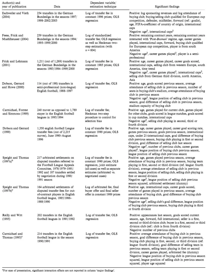
3. Empirical evidence of the determinants of player transfer prices

Several academic articles focused on determining the determinants of football players transfer

prices. These studies’ main findings are best summarized by Fricks (2007) in Table 1 below. This section will focus on the diverging methodologies and the rationale behind the choice of

variables.

Dobson and Gerrard (1999) observe that most research attempting to explain transfer fee

variation between players have focused on four sets of variables; buyer and seller

characteristics, player characteristics and control variables.

The first two sets evolve around club specific characteristics which are used to incorporate the

relative bargaining power of the buying and selling club in the model. The aim is to test if and

how bargaining power plays a role in the transfer market. Variables used in the literature are

reflecting clubs’ financial or sportive power. For example, Carmichael and Thomas (1993) use

9

and selling club’s position in their respective leagues during the season preceding the transfer.

In general, studies using bargaining theory to analyse the determinants of transfer prices have

concluded that the more successful the buyer and selling clubs are financially or in terms of

performance, the higher is the agreed upon price (Fricks, 2007). In addition, the bargaining

power of the selling club is higher than the one of the buying club (Carmichael and Thomas,

1993)

The second category consists of player related characteristics. Researchers have used indirect

proxies of player performance as well as other player characteristics and tested their

relationships to transfer prices. Those include age, playing position on the field, career goals

and number of games played in the previous season. All the research shows that age has a

positive influence on prices and age-squared a negative one. This is due to the fact that a

professional player’s career is characterized by a peak after which performance declines. Goals

are mostly scored by strikers and using it as a measure of performance can bias strikers’ valuation upwards and other player’s downwards. The main problem is that those variables are indirect measures of a player’s contribution to the team (Fricks, 2007). In fact, no studies on the determination of transfer prices have introduced directly observable and position specific

performance measures in their models. Researchers seem to try and alleviate the bias of goals

scored by interacting it with a positional dummy variable. This is done to give goals scored by

player’s others than strikers more importance in the model. The third category pertains to control variables used to correct for time effect when the data covers multiple transfer periods

or seasons.

When it comes to methodologies, researchers either use OLS regressions and/or a Heckman

two step approach. The oldest research papers in Table 1 all used OLS estimations but

Carmichael and al. (1999) argue that samples of transferred players cannot be considered as

10

rather represent sub-populations and suffer from selection bias. To correct for this, Carmichael

and al. (1999) use a Heckman two-step approach which first estimates the probability that a

player gets transferred then uses the ensuing residuals to estimate the transfer fee equation.

However, this method delivers results comparable with OLS estimates but an interesting

finding is that players who get transferred for a higher fee also observed higher transfer

probabilities (Carmichael and al., 1999)

In general, there is consensus in the literature about the influence of selling and buying club

characteristics over the amount of the transfer fee. Yet no studies looked closely at the direct

relationship player performance has with transfer price.

The International Centre for Sport Studies (commonly known under the French acronym CIES)

in Switzerland, more specifically its Football Observatory under the direction of Dr. Rafaele

Poli, has been studying the European football market extensively. Indeed, for several years

now they have been publishing rankings of over- and under-paid football players in the transfer

market among many other reports. Using data on 1500 European transfers over the last five

years, the research centre’s football observatory developed an algorithm which allows the pricing of players according to a series of factors. These factors are performance measured in

goals scored and games played per season over the player’s four past seasons. The level of the

league where the player evolved and the team’s points per game are also taken into account.

International appearances and goals are also considered. They then contrast their results with

11

12

III.

The sample was collected from www.transfermarkt.co.uk. The period under consideration is

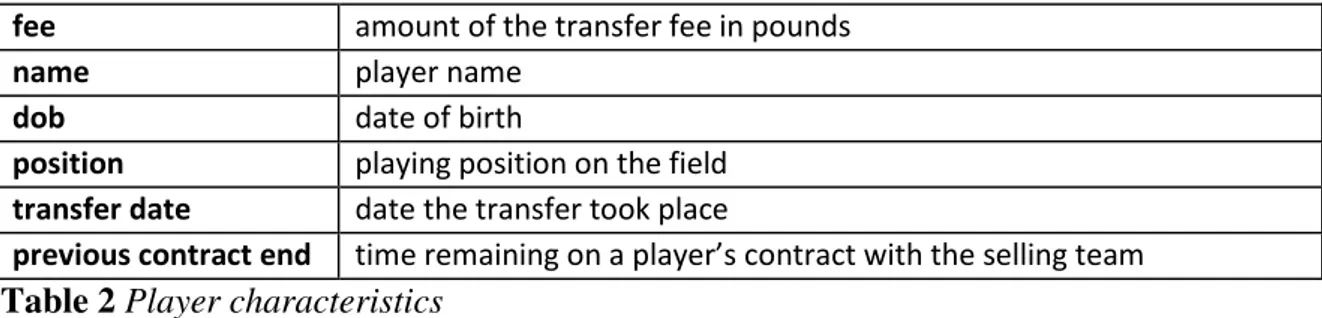
the 2015 summer transfer period which lasted from 1st of July 2015 to 31st of August 2015 for France, Spain, Italy and Germany. In England the transfer period lasts from the 1st of July 2015 to the 1st of September 2015. All players transferred for a fee to or from the Big 5 leagues were gathered with the following information:

fee amount of the transfer fee in pounds

name player name

dob date of birth

position playing position on the field

transfer date date the transfer took place

previous contract end time remaining on a player’s contract with the selling team

Table 2Player characteristics

Observations excluded from the dataset are players who moved as free agents, players sent on

loan by their clubs and young players signing their first professional contract. Performance data

was collected from www.whoscored.com for the remaining players. The performance

measures range across almost all aspects of a footballer’s game.

Apps number of matches started (number of substitutions in a game)

Mins minutes played

Goals goals scored

Assists assists made

SpG shots per game

MotM number of times elected man of the match

Tackles tackles per game

Inter interceptions per game

KeyP key passes per game

Drb3 dribbles made per game

AvgP passes per game Table 3Performance variables

13

A few variables needed to be created using the information gathered. The age of a player at the

time of his transfer was obtained using the date of transfer and the date of birth of a player. The

remaining months on a player’s contract at the time of the transfer was obtained similarly using the expiry date of a player’s previous contract. The number of days between the transfer and

the end of the transfer window, 1st _{September 2015, was also computed. The creation of player}

performance indicators measuring their direct contribution to team effort is explained in the

next section.

Observations for which the data was incomplete were deleted. The resulting dataset includes

137 players used in the subsequent regression.

IV.

Since the existing empirical literature covered bargaining theory extensively, this research will

focus on player performance characteristics as explanatory variables for the determination of

transfer prices in the Big 5 European leagues. Firstly, player performance needs to be defined

and modelled.

1. Player performance

Measuring individual performance in team sports is a complicated matter. Hassan and

Trenberth (2013) identify three problems when attempting to measure individual contributions

in sport team’s efforts. Firstly, the tracking problem which arises with the difficulty to identify,

categorize and enumerate player actions. Secondly, the attribution problem which refers to

14

weighting problem which embodies the difficulty of assessing the significance of different

actions in the determination of match outcomes.

A framework designed by the Football Observatory (of the CIES) to evaluate the performance

of football players according to their roles on the pitch will be used to tackle the first of these

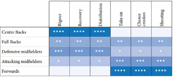
issues. The table below effectively enumerates and categorizes player actions.

Table 4 Key performance indicators according to the CIES Football Observatory (Poli and

al., 2015)

Football players are ranked in five positions and form the rows of Table 4 while individual skill

is broken down into six areas. Rigour refers to strength in duels which here will be measured

by tackles per game. Recovery embodies the ability of players to intercept passes and will be

measured by interceptions per games. Distribution represents the ability to pass the ball

efficiently as to keep possession. It will be measured by passes per game. Take on represents

to ability to challenge opponents to create space and opportunities which will be measured in

dribbles per game. Chance creation is the ability to pass the ball to create scoring opportunities

for team members. It will be measured by key passes. While shooting reflects the ability of

15

the performance indicator each skill will be weighted according to the table above. For

example, for full-backs, each skill will be weighted equally. The final player performance

indicator will be as close as one could get to an observed and direct measure of performance

and was computed for 240 players with complete performance data.

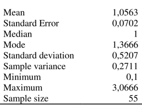
A problem with the performance indicator is that each subsample defined by a player’s position presented different ranges as can be seen in Table 5 below. It prevents performance

comparisons across the whole sample. The best defender has a performance score of 21,3 while

the best forward’s performance is measured at 3.06. Hence the need to normalize each

subsample’s performance score to bring the whole sample on the same scale. Performance

scores are normalised to fit between 0 and 1. The best player at each position has a performance

score of 1 and the worst player of 0.

Full Backs performance indicator Defenders performance indicator

Mean 6,9031 Mean 14,2629

Standard Error 0,3237 Standard Error 0,5869

Median 7,2333 Median 14,8

Mode 8,3166 Mode 16,833

Standard deviation 1,9692 Standard deviation 3,5218

Sample variance 3,8780 Sample variance 12,4031

Minimum 1,95 Minimum 7,5

Maximum 10,183 Maximum 21,3

Sample size 37 Sample size 36

Defensive midfielder performance indicator

Offensive midfielder performance indicator

Mean 10,375 Mean 3,7759

Standard Error 0,4645 Standard Error 0,1906

Median 10,288 Median 3,9777

Mode 8,1555 Mode 5,2333

Standard deviation 3,3173 Standard deviation 1,4887

Sample variance 11,004 Sample variance 2,2164

Minimum 3,2222 Minimum 0,1111

Maximum 17,877 Maximum 7,1777

16

Table 5 Descriptive statistics of positional subsamples.

2. Model specification

Goals scored and assists made are included in the analysis as well as minutes played. They are

expected to have a positive influence over the dependent variable. In addition, the literature did

not yet account for an analysis of the relationship between duration left on a player’s contract before he gets transferred and the transfer fee (Fricks, 2007). The variable “Timerem” will

allow us to investigate this relationship. It is suspected to have a negative relationship with

transfer price since clubs would prefer to sell their player rather than let him walk out for free

at the end of his contract. Date of the transfer is also an interesting variable to be considered

as it can portray the influence of the timing of the transaction on its value. It is expected to have

a positive relationship with the dependent variable to reflect the loss of bargaining power of

the selling club as the transfer deadline approaches. Age is suspected to have a negative

influence over transfer prices as already established in the literature. Minutes played is

expected to show a positive relationship to transfer prices to reflect the added experience that

time on the pitch brings to a player.

The model tested is the following.

Forwards performance indicator

Mean 1,0563

Standard Error 0,0702

Median 1

Mode 1,3666

Standard deviation 0,5207

Sample variance 0,2711

Minimum 0,1

Maximum 3,0666

17

𝐿𝑜𝑔(𝑓𝑒𝑒𝑖) = 𝛽0+ 𝛽1𝑃𝑒𝑟𝑓𝑖 + 𝛽2𝐺𝑜𝑎𝑙𝑠𝑖 + 𝛽3𝐴𝑠𝑠𝑖𝑠𝑡𝑠𝑖 + 𝛽4𝑇𝑖𝑚𝑒𝑟𝑒𝑚𝑖

+ 𝛽5𝑚𝑖𝑛𝑠𝑖+ 𝛽6𝐴𝑔𝑒𝑖 + 𝛽7𝐷𝑒𝑎𝑑𝑙𝑖𝑛𝑒𝑇𝑖𝑚𝑒𝑖+ 𝜀𝑖

Notice the absence of “agesquared”. Including it would allow to incorporate the reversal of the

age effect after a certain threshold representing the loss of value a player is subject to when

approaching the end of his career. It was included in previous trials but was found to be severely

insignificant and hampered the fit of the model. That variable was therefore dropped in this

model. More information about previous trials is available in the appendix file submitted along

with this research. The next section presents the results of the model described above.

V.

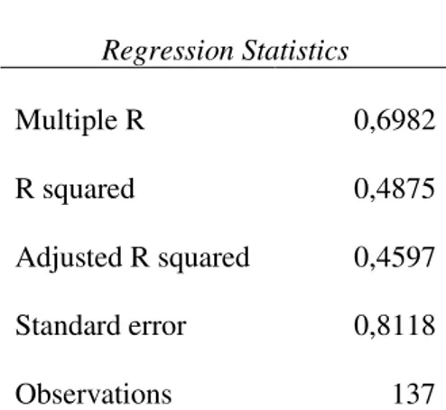
Table 6 below shows the regression statistics and variance analysis of the model. It shows that

the variables in the model explain 46% of the variations in the dependent variables as

represented by the adjusted R-squared. In addition, the F-statistic shows that the joint

significance of the variables of the model is very high. The probability that the results of the

model occurred by chance are close to zero.

(1)

Regression Statistics

Multiple R 0,6982

R squared 0,4875

Adjusted R squared 0,4597

Standard error 0,8118

18

Table 6Regression results

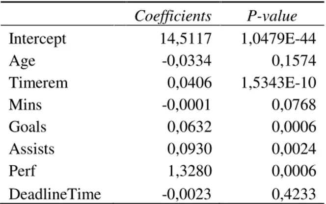
1. Main findings

Table 7 below summarizes the estimated coefficients and their significance. The first striking

result is that when attempting to use performance to explain variations in transfer prices age

has become insignificant at 10% significance level. This result is in striking contrast with all

the results established in the literature.

Coefficients P-value

Intercept 14,5117 1,0479E-44

Age -0,0334 0,1574

Timerem 0,0406 1,5343E-10

Mins -0,0001 0,0768

Goals 0,0632 0,0006

Assists 0,0930 0,0024

Perf 1,3280 0,0006

DeadlineTime -0,0023 0,4233

Table 7 Main findings

Time remaining on player’s contract is the most significant variable of the model and is so at

a 1% significance level. One extra month on a player’s contract is suspected to increase his transfer fee by approximately 4% all else remaining equal. Minutes played show a counter

intuitive result. It is significant at a 10% significance level and shows a negative relationship. ANOVA

df SS MS F

Significance F

Regression 7 80,8999 11,5571 17,5349 3,4678E-16

Residual 129 85,0230 0,6590

19

According to the model an extra minute on the pitch decreases a player’s transfer fee. Even if

the coefficient is incredibly small. Dividing that variable by 90 (minutes in a football game)

and re-estimating the model neither improves it nor the variables coefficient. Goals, as

suspected, is a highly significant variable (significant at a 1% level) and shows a positive

relationship to transfer price. The model estimates that an extra goal increases the price of a

player by 6%. What is surprising is that an extra assist seems to bring about an increase of 9%

in the price. The model predicts that assists are more valuable than goals. That coefficient is

also significant at a 1% level of significance.

The number of days between the transfer date and the transfer deadline appears to be

completely insignificant. The aim was to capture the shift in bargaining power as the deadline

approaches. That effect might depend on other factors such as the willingness of a club to sell

a player. As the deadline approaches, the selling club might drive up the price should the buyer

pursue the player aggressively. On the other hand, it might be that good players get traded at

the beginning of the transfer window and that at the end only average or bad players remain

which would decrease the transfer price over that period. The effects seem more ambiguous

than previously theorized which may explain the insignificance of that variable in this model.

Performance has a positive and significant estimated coefficient. An increase of 0.1 in the

performance score of a player is estimated to increase the transfer fee by 13%. It can thus be

considered as the main determinant of transfer price according to this model since it has the

largest influence given a unit increase.

2. Robustness checks

This section investigates whether the assumption constant variance holds. This is of importance

20

White test for heteroscedasticity was performed and yielded a F-value of 1,3574 which allows

us to not reject the null hypothesis of homoscedasticity (See Appendix 2). Since cross section

data is used, autocorrelation is not an issue in this model.

Another issue which might hamper the reliability of the variable estimates is endogeneity.

Should a variable correlated with both one of the independent variables and with the dependent

variable be omitted from the model then an endogeneity problem occurs. It could be possible

that the performance of a player relative to the rest of his team members is one of those

variables. Should a player’s performance be among the best of his team, this would lead him to be fielded more often hence increasing his minutes on the pitch. In addition, such high

relative performance will decrease his club’s willingness to sell him and increase his transfer price. Since the data gathered does not include measures of relative performance it is

impossible to investigate the issue further but it might explain why the estimate of minutes is

significantly counter intuitive.

3. Interpretation and limitations

The relatively low fit of the model, compared to the studies presented earlier in Table 1, shows

that performance is not as effective as club characteristics at explaining variations in transfer

prices. In addition, when performance is considered, some key variables whose effects were

intuitive and significant in the literature, turn out to be counter intuitive and insignificant. This

may be due to sample characteristics as well as to the number of observations.

The main limitation of the research at hand may be that buyer and seller characteristics were

not investigated jointly with performance. This might explain the relatively low fit of the

model. Incorporating them could picture a more realistic model of the determinants of transfer

21

the manual collection of the data which is extremely time consuming. Another limitation of

this paper, and of the existing literature, is that football players are considered as a labour force.

While in today’s football world it may also be coherent to consider them as financial products.

The data set compiled for this study did present several cases where a player who was loaned

during the 14/15 season was then bought by the club where the loan took place and then sold

at a profit less than two weeks later. Last but not least, the sample contains player transferred

to clubs playing in the Big 5 leagues. Those include players arriving from other continental

federations. It might be more instructive to consider players transferred only within the Big 5.

VI.

This study attempted to establish the relationship between performance and transfer prices paid

for football players transferred to the European Big 5 leagues. Setting the context that football

clubs in Europe are success-maximizers as opposed to profit-maximizers, demand for quality

players should be high and competition to get them fierce. A performance indicator is computed

per position and normalised to enable cross-position comparisons. The model finds evidence

that player performance is an important determinant of transfer prices and has the largest effect.

Another key finding is that the influence of the remaining months on player contract is positive.

Despite the results, further research is needed to combine bargaining theory and performance

into a realistic model of the determinants of transfer prices. In addition, these researches could

focus on the effect of the timing of the transaction on its value as the effects seem ambiguous.

Another interesting angle would be to consider player performance relative to their teammates

22

VII.

Carmichael, F., Forrest, D. & Simmons, R. (1999): The Labour Market in Association Football: Who gets Transferred and for how much?, Bulletin of Economic Research, 51 (2), pp. 125-150

Carmichael, F. & Thomas, D. (1993): Bargaining in the transfer market: theory and evidence,

Applied Economics, 25 (12), pp. 1467-1476

Feess, E. & Muehlheusser, G. (2003): The Impact of Transfer Fees on Professional Sports: An Analysis of the New Transfer System for European Football, Scandinavian Journal of Economics, 105 (1), pp. 139-154 18

Feess, E. & Muehlheusser, G. (2002): Transfer fee regulation in Europe, European Economic Review, 47 645–668

Frick, B. (2007): The Football Players’ Labor Market: Empirical Evidence from the Major

European Leagues, Scottish Journal of Political Economy, 54 (3)

Garcia-del-Barro, P. & Szymanski, S. (2006): Goal! Profit Maximization and Win Maximization in Football Leagues, IASE Working Paper no. 06-21

Leach, S., Szymanski, S. (2015) Making money out of football, Scottish Journal of Political Economy, DOI:10.1111/sjpe.12065, Vol. 62, No. 1, February 2015

Muehlheusser, G. & Feess, E. (2002): Transfer Fee Regulations in European Football, IZA Discussion Paper No. 423.

Poli, R., Ravenel, L., Besson, R., (2015a), Performance analysis: Best clubs and players of the big-5 league season, CIES Football Observatory Monthly Report, Issue no.5 – May 2015 Poli, R., Ravenel, L., Besson, R., (2015b), Transfer expenditure and results, CIES Football Observatory Monthly Report, Issue no.3 – March 2015

Sloane, P.J. (1969): The Labour Market in Professional Football, British Journal of Industrial Relations, July, pp. 181-199

Sloane, P.J. (1971): The Economics of Professional Football: The Football Club as a Utility Maximiser, Scottish Journal of Political Economy, June, pp. 121-146 50

Szymanski, S. & Smith, R. (1997): The English Football Industry: Profit, Performance and Industrial Structure, International Review of Applied Economics, 11 (1), pp. 135-154

Trenberth, Linda & Hassan, David (2013) Managing the Business of Sport: An Introduction

23

Appendices

1) Residual analysis

Observatio n

Predicted

ln(fee) Residuals

residuals squared

Observatio n

Predicted

ln(fee) Residuals

residuals squared

24

42 15,0877128 -0,46127206 0,21277191 110 16,5592071 0,43435728 0,18866624 43 15,2310336 0,08855431 0,00784187 111 15,0386679 -0,17583831 0,03091911 44 15,8566208 1,10519486 1,22145567 112 16,1887219 1,47437976 2,17379566 45 16,7267026 -0,20314181 0,04126659 113 14,3227613 -0,53256859 0,2836293 46 15,4555721 -0,13598415 0,01849169 114 15,1656422 -0,2515194 0,06326201 47 14,6538454 0,560382 0,31402798 115 15,1145602 0,89817498 0,80671829 48 14,5629867 0,91075198 0,82946917 116 16,3373381 -0,66865945 0,44710546 49 14,7501964 -1,57904289 2,49337646 117 15,21185 -1,14947932 1,3213027 50 14,9786593 -0,03821913 0,0014607 118 15,8273784 -0,22010835 0,04844768 51 16,1484156 -0,17766052 0,03156326 119 14,4865256 0,29596881 0,08759754 52 16,2511874 0,67783848 0,459465 120 14,1264582 0,43098974 0,18575216 53 15,8551073 0,38077135 0,14498682 121 15,4242921 0,40612146 0,16493464 54 15,6305605 0,66985675 0,44870806 122 15,5789371 0,43379801 0,18818071 55 15,8032891 -0,66602267 0,44358619 123 14,9450293 0,98069448 0,96176167 56 15,0542283 -0,78129293 0,61041864 124 16,407638 0,01056221 0,00011156 57 15,4518545 0,78402418 0,61469392 125 14,191417 0,25536532 0,06521145 58 14,8795288 -0,51589684 0,26614955 126 15,3403244 -0,42620159 0,1816478 59 15,5538813 0,4588538 0,21054681 127 15,0711672 0,53610283 0,28740624 60 13,7727415 0,09155926 0,0083831 128 14,8526082 1,44780905 2,09615103 61 14,1734889 -1,15648605 1,33745998 129 14,7708385 -0,14439774 0,02085071 62 15,0410929 -0,41465209 0,17193635 130 15,4072069 0,54601412 0,29813142 63 15,391988 0,53373572 0,28487382 131 14,8026786 -0,02018423 0,0004074 64 16,7124608 -0,69972565 0,48961598 132 15,5337986 -0,06005993 0,00360719 65 15,8442616 -0,013848 0,00019177 133 15,220667 -0,18728068 0,03507405 66 16,3581082 -0,34537311 0,11928259 134 16,3406168 0,02042501 0,00041718 67 14,1940819 -1,02292838 1,04638248 135 15,4564739 0,0172647 0,00029807 68 15,1637188 -0,71693646 0,51399789 136 14,9622528 1,19794408 1,43507001 137 14,7445878 0,24340493 0,05924596

2) White’s test

White's test

Regression statistsics Multiple R 0,14091763 R-squared 0,01985778 Adjusted

R-squared 0,00522879 Standard

error 0,80844483 Observations 137

ANOVA

df SS MS F

Valeur critique de

F Regression 2 1,77438208 0,88719104 1,35742664 0,26083721 Résidus 134 87,580128 0,65358304