www.atmos-chem-phys.net/11/1117/2011/ doi:10.5194/acp-11-1117-2011
© Author(s) 2011. CC Attribution 3.0 License.
Chemistry
and Physics
The European aerosol budget in 2006
J. M. J. Aan de Brugh1,2, M. Schaap2, E. Vignati3, F. Dentener3, M. Kahnert4, M. Sofiev5, V. Huijnen6, and M. C. Krol1,7
1Meteorology and Air Quality Section, Wageningen University, Wageningen, The Netherlands
2TNO, Earth, Environment and Life Sciences, research group Climate, Air and Sustainability, Utrecht, The Netherlands 3European Commission, Joint Research Centre, Institute for Environment and Sustainability, Ispra, Italy
4Swedish Meteorological and Hydrological Institute, Norrk¨oping, Sweden 5Finnish Meteorological Institute, Helsinki, Finland
6Royal Netherlands Meteorological Institute, De Bilt, The Netherlands 7Institute for Marine and Atmospheric Research Utrecht, The Netherlands
Received: 28 June 2010 – Published in Atmos. Chem. Phys. Discuss.: 8 September 2010 Revised: 17 January 2011 – Accepted: 27 January 2011 – Published: 9 February 2011
Abstract. This paper presents the aerosol budget over Eu-rope in 2006 calculated with the global transport model TM5 coupled to the size-resolved aerosol module M7. Compar-ison with ground observations indicates that the model re-produces the observed concentrations quite well with an ex-pected slight underestimation of PM10 due to missing
emis-sions (e.g. resuspension). We model that a little less than half of the anthropogenic aerosols emitted in Europe are exported and the rest is removed by deposition. The anthropogenic aerosols are removed mostly by rain (95%) and only 5% is re-moved by dry deposition. For the larger natural aerosols, es-pecially sea salt, a larger fraction is removed by dry processes (sea salt: 70%, mineral dust: 35%). We model transport of aerosols in the jet stream in the higher atmosphere and an import of Sahara dust from the south at high altitudes. Com-parison with optical measurements shows that the model re-produces the ˚Angstr¨om parameter very well, which indicates a correct simulation of the aerosol size distribution. How-ever, we underestimate the aerosol optical depth. Because the surface concentrations are close to the observations, the shortage of aerosol in the model is probably at higher alti-tudes. We show that the discrepancies are mainly caused by an overestimation of wet-removal rates. To match the obser-vations, the wet-removal rates have to be scaled down by a factor of about 5. In that case the modelled ground-level con-centrations of sulphate and sea salt increase by 50% (which deteriorates the match), while other components stay roughly
Correspondence to: J. M. J. Aan de Brugh (joost.aandebrugh@wur.nl)
the same. Finally, it is shown that in particular events, im-proved fire emission estimates may significantly improve the ability of the model to simulate the aerosol optical depth. We stress that discrepancies in aerosol models can be adequately analysed if all models would provide (regional) aerosol bud-gets, as presented in the current study.
1 Introduction
Aerosols have a large impact on the behaviour of our atmo-sphere as they influence the earth’s radiation budget both di-rectly through interaction with solar radiation (Hess et al., 1998; Haywood and Boucher, 2000; IPCC, 2007) and indi-rectly through altering the properties and life cycle of clouds (Rosenfeld et al., 2008; Kaufman et al., 2002). The aerosol-climate interactions are complex and the aerosol forcing is much less certain compared to the radiative effect of green-house gases. Hence, the combined direct and indirect aerosol effect may have masked the climate sensitivity towards an in-crease in greenhouse gases to an unknown extent (Anderson et al., 2003).
Exposure to particles has been associated with adverse health effects and particles are believed to be the most impor-tant air polluimpor-tant responsible for these health effect. Short-term exposure has been associated with increased human morbidity and mortality (Brunekreef and Holgate, 2002; Dockery et al., 1993; Pope et al., 1995). Although most health studies have quantified relationships between the total aerosol mass (PM10or PM2.5) and health effects, some
(Hoek et al., 2002) and particle size (Stone and Donald-son, 1998) might play a significant role. To reduce the ad-verse health effects, air quality standards for particulate mat-ter have been implemented in many countries. To design ef-fective mitigation strategies, governments need to know the relationship between sources and concentrations of particu-late matter. Within Europe, these relationships are tradition-ally obtained through source-receptor calculations (Seibert and Frank, 2004). Another way to investigate these relation-ships is a budget analysis as pointed out in this paper.
To better understand the relationship between the emis-sion of aerosols and their precursors on the one hand, and the observed distribution of aerosols on the other hand, numeri-cal models have been developed that describe the aerosol life cycle (Wilson et al., 2001; Bauer et al., 2008; de Meij et al., 2006). This presents an extremely challenging task as one needs to accurately model a host of sources, formation and transformation pathways as well as removal processes to as-sess aerosol composition, size distribution and mixing state. Together they determine the optical properties of aerosols as well as their ability to act as cloud condensation nuclei (CCN). Thus, to describe the full life cycle of aerosols one needs reliable (size-resolved) emission inventories and pa-rameterisations to supply the necessary boundary conditions for the models (Vignati et al., 2010a; Dentener et al., 2006). Furthermore, one needs to represent the complex aerosol dy-namics (Stier et al., 2005; Vignati et al., 2004; Wilson et al., 2001; Lee and Adams, 2010; Korhonen et al., 2008). Also, it is necessary to couple the aerosol dynamics to atmospheric chemistry to account for secondary aerosol formation, semi-volatile species and the involvement of aerosols in numerous chemical cycles. Finally, one needs to consider size and com-position resolved aerosol removal by wet and dry decom-position processes. In the assessment of the aerosol budget, the key uncertainties arise from inaccurate emission estimates (Den-tener et al., 2006; Vignati et al., 2010b) and uncertainties in the wet-removal process (Chin et al., 2000).
In a model intercomparison study, Textor et al. (2006) highlighted the poor agreement among models concern-ing aerosol processes, and specifically the wet removal of aerosols. The parameterisations in models are probably of-ten tuned to produce a reasonable comparison with (satellite) observations. Unfortunately, model specific tuning often re-mains undocumented and arbitrarily tuning of models can have led to the huge diversity in the analysed simulations. Textor et al. (2006) showed that methodologies to analyse and compare different models are indispensable to improve our ability to model the aerosol distribution. One method that provides details about the processes that matter for aerosol modelling is a budget analysis. Budget analysis also helps to understand differences between models. An aerosol budget analysis with a bulk aerosol approach has been described in Kanakidou (2007).
The aim of this paper is threefold. First, we will present a description of the TM5 model coupled to the size-resolved
aerosol module M7 and compare model results with obser-vations. Second, we will analyse the European aerosol bud-get and quantify the aerosol import and export terms in the boundary layer and the free atmosphere. Thirdly, we will highlight some uncertainties that are associated with aerosol modelling. Specifically, we will address the wet-removal parameterisation in our model and focus on an anecdotical improvement of the fire-related emissions during a biomass burning episode in April–May 2006 in Eastern Europe.
2 Model and measurements
The quantification of the aerosol budget over Europe is per-formed with the global transport model TM5 (Krol et al., 2005) coupled to the aerosol dynamics module M7 (Vignati et al., 2004). To calculate the aerosol budget in the model, Europe is defined from 34◦N to 62◦N and from 12◦W to 36◦E. We examine the import, export, emission and deposi-tion of aerosols as well as chemical processes that influence particulate matter. Below we describe the main characteris-tics of the model with a focus to the aerosol description as well as the observations used for evaluation.
2.1 TM5 model description
The global horizontal resolution of the offline chemistry transport model TM5 is 6◦longitude by 4◦latitude. The ver-tical grid comprises 25 hybridσ-pressure levels ranging from surface up to in the stratosphere. As the region of interest is Europe, we used TM5’s two-way nested zoom capability (Krol et al., 2005; Berkvens et al., 1999) to acquire a higher resolution over Europe. The zoomed region is defined from 12◦N to 66◦N and from 21◦W to 39◦E, with a resolution of 1◦×1◦. Note that our definition of Europe to calculate the budget is only a part of this zoomed region. A transitional zone from 2◦N to 74◦N and from 36◦W to 54◦E, with a resolution of 3◦×2◦is used to smoothen the transition (Krol et al., 2005). The vertical resolution remains the same.
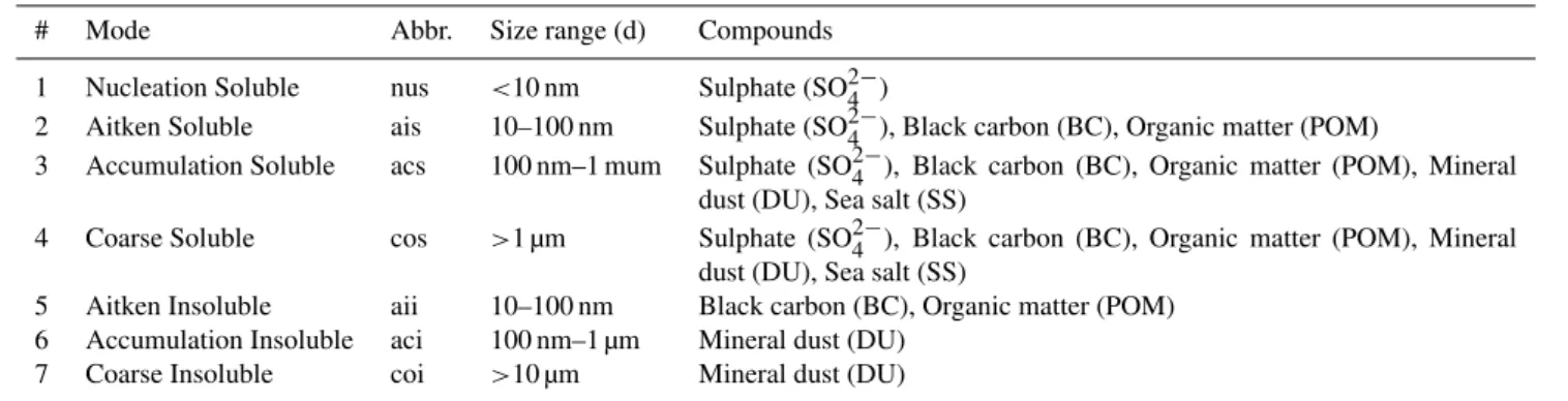
Table 1.The seven modes in M7, their solubilities, size ranges and chemical compounds.
# Mode Abbr. Size range (d) Compounds
1 Nucleation Soluble nus <10 nm Sulphate (SO24−)
2 Aitken Soluble ais 10–100 nm Sulphate (SO24−), Black carbon (BC), Organic matter (POM)
3 Accumulation Soluble acs 100 nm–1 mum Sulphate (SO24−), Black carbon (BC), Organic matter (POM), Mineral dust (DU), Sea salt (SS)
4 Coarse Soluble cos >1 µm Sulphate (SO24−), Black carbon (BC), Organic matter (POM), Mineral dust (DU), Sea salt (SS)
5 Aitken Insoluble aii 10–100 nm Black carbon (BC), Organic matter (POM) 6 Accumulation Insoluble aci 100 nm–1 µm Mineral dust (DU)
7 Coarse Insoluble coi >10 µm Mineral dust (DU)
(Krol and van Weele, 1997; Landgraf and Crutzen, 1998). The version used is subversion (SVN) revision 2887.
2.2 Aerosol module description
All aerosol processes including wet and dry removals are calculated in the model using the size resolved number and masses given by the aerosol dynamics module M7 (Vignati et al., 2004).
2.2.1 Aerosol dynamics
During the chemistry step of TM5, M7 is called to simulate the aerosol microphysics. M7 distinguishes seven classes (modes) of aerosols of different size and solubility. The prop-erties of M7’s aerosol modes are listed in Table 1. There are four size classes for soluble aerosols and three for insolu-ble aerosols. Chemical compounds can be present in various modes. For each mode, one number tracer and several trac-ers for the chemical compounds are subject to transport in the model for a total of twenty-five tracers.
M7 considers the modes as log-normal size distributions (von Salzen, 2006) with defined median radius (r) and spread (σ). Although aerosols may not be spherical, they are as-sumed spherical in the model. The size distribution of a mode looks like (Seinfeld, 1986):
dN d lnr =
N
√
2π lnσ · e
−(lnr2 ln2−lnσr)2 (1)
Here,ris the size,N is the total aerosol number concen-tration,ris the median radius andσis the geometric standard deviation.
A mode consists of a number concentration and several component masses that are internally mixed (N,[M]) (Stier et al., 2005). Given the modal component masses and their densities, the total volume (V) can be calculated. This vol-ume is represented by a log-normal distribution as in Eq. (1). To derive this distribution, M7 assumes a constant standard deviation, which allows the volume per aerosol (NV) to de-termine the median radius (r). The standard deviation is set
to 2.00 for the coarse modes and to 1.59 for the other modes (Vignati et al., 2004). The medianr is given by (Seinfeld, 1986):
r= 3
r 3V
4π Ne
−9 ln22 σ (2)
M7 handles the formation of new particles (binary nucle-ation) (Vehkam¨aki et al., 2002), the coagulation of particles and the condensation of sulphuric acid to existing particles. M7 ensures that the modes keep their inherent solubility by moving coated particles to the soluble (mixed) mode. The size classes are preserved by transferring mass of growing aerosols to the next mode. M7 diagnostically calculates the water attached to the soluble particles (Vignati et al., 2004).
2.2.2 Ammonium and nitrate
In Table 1, two compounds that are important for the aerosol budget over Europe (Putaud et al., 2004) are missing: am-monium (NH+4) and nitrate (NO−3). Observations show that nitrate is very abundant, especially in the western European cold season (Schaap et al., 2002; Mehlmann and Warneck, 1995). There is a temperature-dependent equilibrium be-tween gas phase nitric acid (HNO3) and nitrate, dissolving
into and evaporating out of the aerosol. This equilibrium also depends on the available aerosol sulphate (SO24−) and gas phase ammonia (NH3). M7 is not designed to model
aerosol associated water mass, can be sufficiently accurately reproduced by EQSAM with respect to other global model uncertainties (Metzger et al., 2002b).
2.2.3 Dry deposition
While gas-phase chemicals exhibit diffusive dry deposition (Ganzeveld et al., 1998; Hicks et al., 1986), aerosols are re-moved by diffusive dry deposition and gravity-driven sed-imentation (Slinn and Slinn, 1980; Kerkweg et al., 2006). Both deposition pathways depend on the size of the aerosols. To calculate the deposition velocities for the tracers in each mode, the lognormal distribution is used to distribute the mass and number tracers into twenty-three size bins. Each of these bins is subject to a bin-dependent deposition velocity, recalculated every three hours depending on e.g. atmospheric stability and surface type (Ganzeveld et al., 1998).
After accounting for dry deposition in each bin, the log-normal distribution is reconstructed. For simplicity, the modes remain log-normal with a fixed standard deviation. Hereby, aerosol mass moves from a size range with a slower deposition velocity to a size range with a faster deposition velocity. This introduces a bias that hard to avoid, but might accelarate loss by deposition.
Apart from surface deposition, the coarse mode aerosols exhibit a non-negligible fall velocity due to gravitational settling in the atmosphere. This sedimentation process is modelled by calculating 3-D fields of the fall velocities for each mode (Slinn and Slinn, 1980). Sedimentation removes preferably the larger particles, which results in smaller fall velocities for the aerosol numbers than for aerosol masses. The sedimentation process also changes the median radii of the M7 modes.
2.2.4 Wet deposition
Wet deposition is split in deposition from stratiform and con-vective precipitation. For stratiform precipitation, in-cloud scavenging and below-cloud scavenging is handled sepa-rately. Below-cloud scavenging of gases is linearly related to the surface rain flux, using a gas-to-droplet transfer coef-ficient based on the Reynolds and Sherwood numbers of the falling rain droplets. For aerosols, the scavenging parameter-isation from Dana and Hales (1976) is used and calculated for each aerosol mode separately. In-cloud scavenging is mod-elled in two phases: the mass transfer of soluble gases and aerosol to the liquid phase and the formation of rain droplets (Roelofs and Lelieveld, 1995). In convective precipitation, aerosols are assumed to be removed very efficiently (similar to HNO3). The removal rate is modelled as a simple function
that depends on the convective precipitation at the surface (Vignati et al., 2010b).
TM5 assumes well-mixed grid cells. However, the time scale of wet removal can become faster than the mixing time scale of the grid cell. Therefore, the wet-deposition
yield will increase for larger grid boxes. This is a signifi-cant issue as multiple resolutions are used within the same simulation. This issue is treated pragmatically by introduc-ing a time paramter τnomix, in which the in-cloud,
below-cloud and below-cloudless fractions of a grid cell are treated quasi-independently (Vignati et al., 2010b). This way, the wet re-moval in large grid cells is slowed down, reducing the reso-lution dependence. Applying the wet removal on a fraction of the gridbox has always been a challenge for modellers, as outlined in a study on210Pb (Balkanski et al., 1993).
2.2.5 Emission
Emission data used in the model are those recommended for the AEROCOM (Dentener et al., 2006) model intercompar-ison studies and from the IPCC (IPCC, 2000). For biomass burning emissions, we use climatologic inventories from the global fire emission database (GFED 2) (Randerson et al., 2006; van der Werf et al., 2006) with prescribed height distri-bution (Dentener et al., 2006). In these data, it is predefined in which modes the aerosols are emitted. Aerosol mass emis-sions have an assumed lognormal distribution with a median radius (r) (Table 2) in their inventories. This median radius is used to calculate the total emitted aerosol number with a mode-dependent standard deviation.
Ammonia is emitted mainly by domestic animals and syn-thetic fertilisers. Other sources of ammonia are biomass burning, the oceans, crops, human population and pets and natural soils (Bouwman et al., 1997).
Oxidised sulphur is emitted by industry, fossil fuel com-bustion (Cofala et al., 2005), biomass burning (Randerson et al., 2006; van der Werf et al., 2006) and volcanoes (An-dres and Kasgnoc, 1998; Halmer et al., 2002). Part (2.5%) of the sulphur is emitted directly in the particulate form (SO24−) (Stier et al., 2005; Dentener et al., 2006). The particulate sul-phate emissions from biomass burning and fossil fuel com-bustion are divided equally over the Aitken and accumulation mode, while industrial sulphate emissions are all in the accu-mulation mode (Dentener et al., 2006).
Table 2.Implemented aerosol emissions with the predefined M7 modes and median emission radii.
Compound Category Percentage Mode Median radius (µm)
SO24− Fossil fuel (Domestic and road transport) 50 ais 0.03 SO24− Fossil fuel (Domestic and road transport) 50 acs 0.075
SO24− Biomass burning 50 ais 0.03
SO24− Biomass burning 50 acs 0.075
SO24− Industry 100 acs 0.075
BC Fossil fuel 100 aii 0.015
BC Biomass burning 100 aii 0.04
POM Fossil fuel 65 ais 0.015
POM Fossil fuel 35 aii 0.015
POM Biomass burning 65 ais 0.04
POM Biomass burning 35 aii 0.04
POM Secondary organic aerosol 100 ais 0.01∗
DU Wind blown ∗∗ aci ∗∗∗
DU Wind blown ∗∗ coi ∗∗∗
SS Wind blown ∗∗ acs 0.08
SS Wind blown ∗∗ cos 0.63
∗SOA is assumed to condensate on existing aerosols so particle numbers are only created when needed to prevent unrealistic situations. ∗∗Emissions in different modes are independent.
∗∗∗Variable radius, included in the AEROCOM emission file.
organic matter involved in nucleation has been coagulated efficiently. Furthermore, through coagulation of the Aitken mode particles, we mimic the condensation of these organic compounds to the accumulation mode.
For dust, we used pre-calculated AEROCOM data (Den-tener et al., 2006). The emission sizes are variable and are pre-calculated as well. Dust is emitted both in the insoluble accumulation mode and the Insoluble coarse mode. Sea salt emissions are calculated online as function of the ten-meter wind speed as described in Vignati et al. (2010a) and Gong (2003). Sea salt is emitted in both the soluble accumulation mode and the soluble coarse mode.
2.2.6 Aerosol optics
We calculate the AOD in our model from the aerosol concen-trations using Mie scattering theory (Mie, 1908; Barber and Hill, 1990). An aerosol contributes to the AOD, depending on its wet radius (rw), its complex refractive index (m) and the wavelength (λ).
The size of the wet droplets (rw) is calculated from the me-dian wet radius (rw) and the fixed standard deviation (σ). The
refractive index (m) of aerosol compounds, including wa-ter, are based on ECHAM-HAM (Kinne et al., 2003), OPAC (Hess et al., 1998) and Segelstein (Segelstein, 1981).
We compute for each time step, for each grid cell and for each aerosol mode an effective refractive index based on the chemical composition. We do not employ a sim-ple volume-weighted mean of the refractive indices of the chemical compounds, which is known to give inaccurate re-sults. Rather, we use proper effective medium theory from
Maxwell-Garnett (Maxwell-Garnett, 1904) and Bruggeman (Bruggeman, 1935).
Mie-scattering calculations demand a significant compu-tational burden and simplifying the Mie-scattering theory causes significant errors (Boucher, 1997). To tackle this problem, we pre-calculated a lookup table. The input param-eters of this lookup table (refractive index and size) are sam-pled with forty times fifteen values for the refractive index (real×imaginary) and a hundred values for the size parame-terrw
λ. With interpolation, the discretisation error is expected
to be low (at most a few percent).
By calculating the AOD at several wavelengths, we can de-termine the ˚Angstr¨om parameter (Russell et al., 2010) with the following general relationship between AOD and wave-length ( ˚Angstr¨om, 1929):
τ =βλ−α (3)
Here,τ is the AOD,βis a prefactor,λis the wavelength and
αis the ˚Angstr¨om parameter. The prefactorβ is a measure for the overall AOD and the ˚Angstr¨om parameter is a mea-sure for the wavelength-dependence of the AOD. Verifica-tion on the ˚Angstr¨om parameter enables to check whether the aerosol distribution is dominated by fine (α>1.3) or coarse (α<1.3) particles.
2.3 In-situ measurements
yearly averaged data for particulate matter, aerosol composi-tion and aerosol precursors. The averaged data for 2006 were used for the stations that produced valid data during at least 10% of the time. For the vast majority of the used data points (94%), this valid-data percentage was above 50%. Verifica-tion of the model results against measurements for PM and its components is hampered by potential artefacts in the sam-pling. PM filter measurements are uncertain due to poten-tial losses of ammonium nitrate and absorption of nitric acid and organic compounds (Vecchi et al., 2009). The above-mentioned volatilisation and absorption artefacts cause the sampling of nitrate and ammonium to be difficult (Yu et al., 2006; Zhang and McMurry, 1992; Cheng and Tsai, 1997). Correct sampling is only possible with denuder filter packs. However, these labour intensive methods are hardly used in Europe (Schaap et al., 2002). Hence, we use aerosol nitrate and ammonium data from inert filters, although we acknowl-edge that they are prone to losses at temperatures above 20◦C (Schaap et al., 2004b). Most data on nitrate and ammonium, however, are given as the sum of gas and aerosol concentra-tion. Gas phase concentrations for ammonia and nitric acid obtained with a filter pack are used here when reported by EMEP.
Observations of sulphur and nitrogen compounds are re-ported as masses S and N rather than total mass. Sea-salt concentrations are evaluated with observed sodium (Na) con-centrations. Throughout this paper, we will express any sul-phur compounds, nitrogren compounds or sea salt as masses S, N and Na. For the conversion of total sea salt to sodium, we use a conversion factor of 0.306 (Millero, 2004).
Unfortunately, measurements of carbonaceous compounds of 2006 are very scarce. Therefore, we will use measure-ments from the EMEP EC-OC campaign in 2002–2003 (Yt-tri et al., 2007). In the EMEP campaign, organic carbon (OC) is measured, while TM5 simulates organic matter (POM). In the analysis, a factor 1.4 is used to convert the observations of organic carbon to organic matter to account for the non-carbon part of the organic matter.
There are also insufficient observations of mineral dust aerosol. Mineral dust is a mixture of many components, so it is very difficult to measure it reliably, especially when only a small fraction of the total aerosol mass is dust, which is the case in the majority of Europe.
We compare the modelled aerosol optical depth (AOD) to European observations from the Aerosol Robotic Network (AERONET) (Holben et al., 2001). These are measured by the sun-powered CMEL Electrique 318A specral radiometer that points systematically to the sun in a programmed routine (http://aeronet.gsfc.nasa.gov).
In the model, the AOD is calculated at the wavelengths (λ) at which the AERONET stations measure. We sample the observed AOD-values with 1.5-h intervals, where multiple measurements within one interval are averaged. This adapts the time resolution of the observations to that of the model.
We also analyse the ability of the model to simulate the ˚
Angstr¨om parameter. The ˚Angstr¨om paramter is reported by AERONET as well. In our model, we use a function fit of Eq. (3) to obtain the ˚Angstr¨om parameter.
3 Results and discussion
In this section, we first examine the modelled surface con-centrations of the aerosol components and precursor gases in Europe, as well as AOD and ˚Angstr¨om parameter. Next, we compare these results with observations followed by the European budget of aerosol compounds and precursors. To address the model’s ability to simulate the full aerosol bur-den we evaluate the modelled AOD and ˚Angstr¨om parameter with observations. Finally, we will address two main uncer-tainties, namely wet removal and biomass burning emissions.
3.1 Concentration distribution
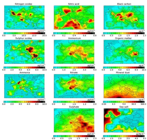
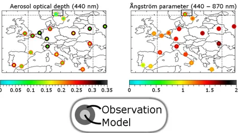
The annual average concentration distribution of aerosol chemical compounds and their precursors are shown in Fig. 1. The AOD and the ˚Angstr¨om parameter are shown in Fig. 2.
Nitrogen and sulphur oxides show a hot-spot structure with high concentrations in industrialised regions with SOx
(SO2, H2SO4) more in Eastern Europe and NOy(NO, NO2,
NO3, HNO4, N2O5, PAN) more in the Western Europe. We
clearly model an ammonia hot spot in the Netherlands, which is due to high population of livestock (Buijsman et al., 1987). Nitric acid shows high concentrations over sea. In reality, ni-tric acid may react with sea salt and displace chloride (Glas-gow, 2008; Schaap et al., 2004a). This reaction is not imple-mented in the model, since it has only a small effect on the aerosol distribution over land.
In contrast to primary gaseous pollutants, secondary inor-ganic aerosols have smoother distributions as they are of sec-ondary origin. The ammonium concentration shows features of both nitrate, which peaks in north-western Europe and in the Po Valley, and sulphate, which shows highest concen-trations in south-eastern Europe. This is because both nitric acid and sulphuric acid are neutralised by ammonium.
Primary anthropogenic carbonaceous aerosols show high concentrations in densely populated and industrialised re-gions. As for primary gaseous pollutants (NOy and SOx),
this results in a hot-spot structure. For black carbon and or-ganic matter, the hot spots are located at different positions. However, the hot spot structures of NOy and black carbon
only differ slightly (more NOy in England and more black
carbon in Poland).
Fig. 1. Modelled surface concentrations of the aerosol tracers and precursor gases. Note that the colour scale used for mineral dust is logarithmic. Nitrogen oxides include NO, NO2, Peroxyacytyl nitrate (PAN), NO3, HNO4and N2O5, but no nitric acid or aerosol nitrate.
Sulphur oxides include SO2and H2SO4, but no aerosol sulphate. All values are averaged over 2006.
Fig. 2.Modelled optical properties of the atmospheric column averaged over 2006.
open sea. Above land, significant sea salt-concentrations are only present in coastal areas.
The calculated annual mean AOD is highest in the south and south-eastern Europe with values above 0.15. Mineral dust and sulphate appear to be the most dominant contribu-tors to the AOD, since the AOD is high at locations where mineral dust or sulphate is abundant (see Figs. 1 and 2). The
˚
Angstr¨om parameter is low over the sea and over northern Africa, because sea salt and desert dust are mostly coarse mode aerosols. Over land, the fine anthropogenic aerosols dominate, resulting in high ˚Angstr¨om parameters.
3.2 Model evaluation
Model results of particulate matter compounds and precursor gases have been compared with in-situ observations. When comparing with size-segregated observations (e.g. PM10),
the log-normal distribution of M7 is used to calculate which fraction of the modelled aerosol mass is below the size limit. First, we will compare annually averaged concentrations. Later on, we will analyse a few time series of PM10for
3.2.1 Annual means
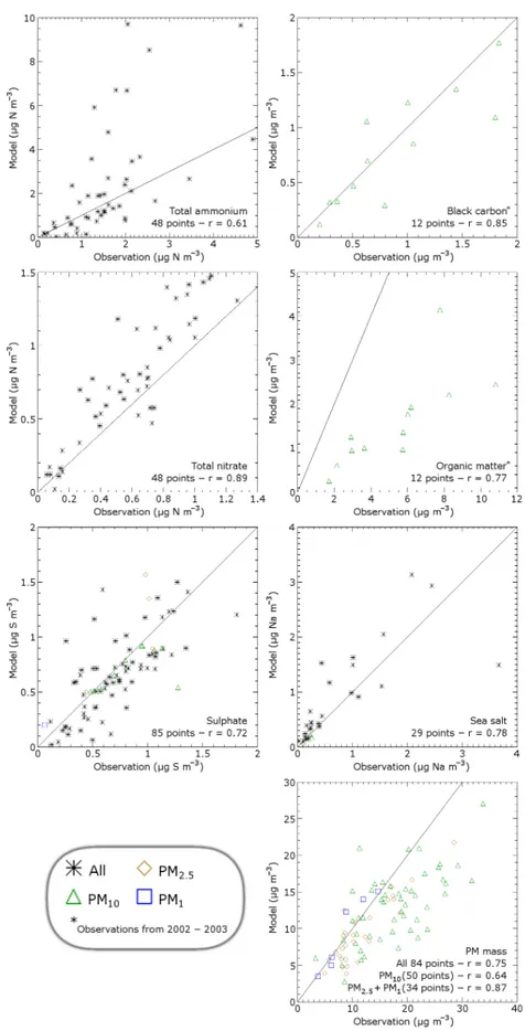
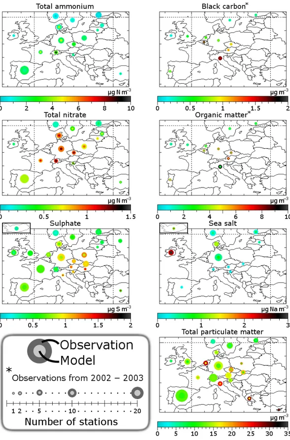
The most important results of the comparison of annually averaged aerosol and precursor concentrations are shown in Fig. 3. Figure 4 shows the results per country represented in a graphic way.
Total reduced nitrogen (ammonia and ammonium) is slightly overestimated. Aerosol ammonium is represented quite well, but ammonia is overestimated. It is well-known that modelling ammonia is challenging due to the impor-tance of local effects (Dentener and Crutzen, 1994). Still, the Dutch ammonia hot spot is caught remarkably well in the model. Interestingly, TM5 overestimates ammonia while many other models underestimate ammonia concentrations (Schaap et al., 2004a). An issue is that the night-time centrations estimated by the model are too high. These con-centrations are very sensitive to the stability of the noctur-nal boundary layer (van Loon et al., 2007). Especially TM5, as a global model, has resolution limitation for the noctur-nal boundary layer, because it is a small-scale phenomenon (∼50 m). Therefore, the nocturnal boundary layer tends to be poorly defined in TM5. This is very important for ammonia, because the modelled emissions are assumed constant over the day (de Meij et al., 2006), which implies that ammonia is emitted into the stable boundary layer, causing night-time accumulation. In reality, ammonia emissions show a con-siderable diurnal variation with peak emissions during the day and even a net night-time surface uptake of ammonia (Wichink Kruit et al., 2007), which may be released during the next day.
The total oxidised nitrogen (nitric acid and aerosol ni-trate) is represented better. There is some overestimation, but the spatial correlation is good (r= 0.89). When considering aerosol nitrate, about the same conclusions could be drawn. However, the modelled concentrations of nitric acid are far off (bad correlation and overestimation by a factor of two). We already addressed that the values above sea are modelled too high because the acid displacement reaction is not taken into account (see Sect. 3.1 and Schaap et al., 2004a; Glas-gow, 2008). This issue may affect modelled concentrations in coastal areas, where many stations are located. Though the nitric acid concentration is the difference between to-tal nitrate and aerosol nitrate (both well represented in the model), nitric acid has higher uncertainties because of higher uncertainties in sampling for nitric acid (see Sect. 2.3). Also, the nitric acid concentrations are often much lower than the aerosol nitrate concentrations, which means that the relative uncertainty becomes higher.
Sulphate is represented quite well. However, there is an overestimation by a factor of two for sulphur dioxide, the precursor of sulphate (not shown). A slow oxidation of sul-phur dioxide may partly explain this discrepancy, but higher oxidation would also lead to higher surface sulphate concen-trations. However, increased in-cloud oxidation at higher al-titudes would be more consistent. The time scale of in-cloud
oxidation of sulphur dioxide is very uncertain (Langner and Rodhe, 1991). Also, the emission heights of sulphur dioxide may play an important role. For instance, the sulphur dioxide emissions from AEROCOM are higher in the lower model levels than those of EMEP, which can cause a surface con-centration discrepancy of a factor of two in eastern Europe (de Meij et al., 2006). Another possibility is that the emis-sion rate of sulphur dioxide is too high in the model or there is an unaccounted or underestimated loss of sulphur dioxide that does not lead to sulphate production, e.g. dry deposition (Chin et al., 2000).
As we mentioned in Sect. 2.3, we compare our modelled results with observations from the EC-OC campaign of 2002 and 2003. Black carbon is represented well, as shown also in Vignati et al. (2010b). There is a huge (factor 3 or more) underestimation of particulate organic matter, though there is a quite okay spatial correlation between observations and model results. Secondary organic aerosols (Volkamer et al., 2006) and resuspended aerosols (Sternbeck et al., 2002), which are rich in organic matter, are significantly underes-timated by TM5. An earlier evaluation of organic matter (Vignati, personal communication, 2010) also shows such an underestimation.
From the comparison of modelled and observed total par-ticulate matter, we can conclude that the aerosol spatial dis-tribution is reproduced reasonably well. There is a slight un-derestimation of the coarse aerosols (PM10) that is probably
due to resuspension of aerosols, which is not included in the model, but may be important for local PM10concentrations
(Sternbeck et al., 2002). Another factor can be an underesti-mation of secondary organic aerosols (Volkamer et al., 2006) or the unaccounted mass (e.g. dust or water) which is fre-quently present in PM10measurements.
The spatial variability of sea salt is represented very well. However, the absolute concentrations are significantly (50%) overestimated, probably due to uncertainties in emissions and the dry deposition parameterisation. A sea salt overesti-mation is also shown in Manders et al. (2010).
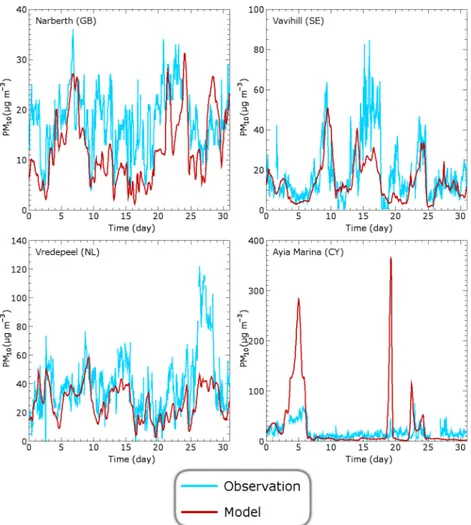
3.2.2 Time series January 2006
To evaluate the ability of TM5 to capture synoptic events, we compare time series of modelled and observed total PM10
for January 2006. Four EMEP stations provide hourly data of PM10for this month. The results are shown in Fig. 5.
We clearly calculate less variability than observed. TM5, as a global model, is unable to simulate local effects of short durations. This is most clearly visible in Narbeth (GB) where TM5 cannot follow the rapid changes in PM10 that
Table 3. European annual budget table of nine tracers for the boundary layer (surface up to 850 hPa), with (B)urden, (L)ifetime; the sinks: (C)hemical reactions, (A)erosol condensation, (D)ry deposition, (W)et deposition, (H)orizontal transport and (V)ertical transport; and the sources: (E)mission, (C)hemical reactions, (A)erosol condensation, (H)orizontal transport and (V)ertical transport. Burdens (Gg) are averages of monthly samples. Lifetimes (days) are burdens divided by total sinks. Fluxes (Gg yr−1) are annual totals. NO
yincludes NO,
NO2, Peroxyacytyl nitrate (PAN), NO3, HNO4and N2O5, but no nitric acid or aerosol nitrate. SOxincludes SO2and H2SO4, but no aerosol
sulphate. Nitrogen compounds are expressed as masses N, sulphur compounds as masses S and sea salt as masses Na.
Boundary layer
Tracer NOy SOx NH3 HNO3 NH4+ NO−3 SO24− BC POM DU SS
B 12.1 18.4 3.2 5.3 7.0 2.0 7.0 2.4 6.8 64.4 8.4
L 0.6 0.7 0.2 0.6 1.7 1.5 2.0 1.6 1.6 1.5 0.3
Sinks
C 3804 487 18
A 564 1535 473
D 1154 5038 3378 1430 39 26 55 11 701 8062
W 863 405 860 604 254 502 142 403 4071 1869
H 421 552 46 329 346 79 410 112 310
V 1567 1780 622 207 585 141 330 268 773 1176
Sources
E 6943 9051 6004 232 547 1541 3931 10 663
C 234 3298 487
A 1535 473 564
H 7853 446
V 4033
Here, resolution plays a big role, because Cyprus is an island as small as a TM5 grid box. Therefore, TM5 models dust storms at Ayia Marina (CY) that are not observed at the sta-tion. Only the broad peak at the beginning is visible in the observations, though with a much smaller magnitude.
3.3 The aerosol budget
For the analysis of the aerosol budget, we split the atmo-sphere over Europe into two parts: the boundary layer (sur-face up to 850 hPa) and the free atmosphere (850 hPa up to top of atmosphere). The budget is split into sources and sinks and the processes: emission (E), chemical reactions (C), aerosol condensation (A), dry deposition (D), wet deposi-tion (W) and the horizontal (H) and vertical (V) transport terms. The vertical transport term denotes the transport of tracer mass between the boundary layer and the free tropo-sphere. Nitric acid also has a stratospheric boundary condi-tion determined by its relacondi-tionship with stratospheric ozone (Santee et al., 1995). The gain or loss due to this boundary condition is counted as vertical transport (V) for the free at-mosphere.
Figure 6 visualises the transport terms and all budget terms are listed in Tables 3 and 4. Note that the lifetimes, especially in the boundary layer, are low because export terms, includ-ing vertical export, are regarded as sinks as well. All budgets close with an accumulation or depletion (difference between sources and sinks) of less than one percent of the budget.
Although only 15% of the air mass is in the boundary layer, the calculated burdens in the boundary layer are
com-parable to those in the free atmosphere. However, the hori-zontal fluxes in the boundary layer are much smaller than in the free atmosphere (see Fig. 6), indicating that the bound-ary layer budget is dominated by emission, deposition and vertical transport. Wet deposition is the major sink of all aerosols, except for mineral dust and sea salt, which exhibit efficient dry deposition because of their large size (see Ta-bles 3 and 4). The numbers in these taTa-bles are raw model results, only rounded to whole gigagrams per year, while the uncertainties are much larger. Given the uncertainties, we will round percentages in the interpretations to multiples of 5%.
We model a net export of all anthropogenic aerosol com-pounds from Europe and a net import of natural aerosol (sea salt and mineral dust). The boundary layer over Europe ex-ports anthropogenic aerosols in all four directions, while in the free atmosphere, Europe imports aerosols and gases from the west due to the jet stream. However, the net horizon-tal export in the free atmosphere is comparable to the export in the boundary layer as a large part of the tracers in the jet stream are not deposited in Europe but pass through the Eu-ropean domain.
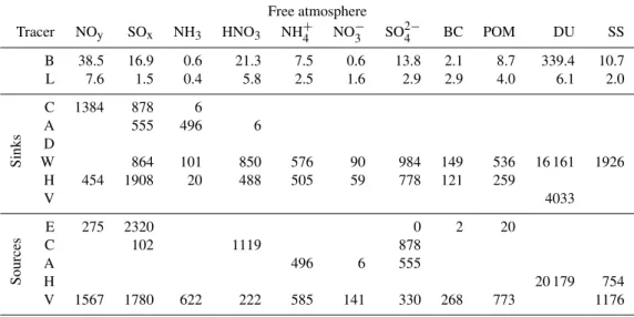
Table 4.European annual budget table of nine tracers for the free atmosphere (850 hPa up to top of atmosphere), with (B)urden, (L)ifetime; the sinks: (C)hemical reactions, (A)erosol condensation, (D)ry deposition, (W)et deposition, (H)orizontal transport and (V)ertical transport; and the sources: (E)mission, (C)hemical reactions, (A)erosol condensation, (H)orizontal transport and (V)ertical transport. Vertical transport includes stratospheric interchange. A value of 0 in the table means a value below 0.5 (rounded down to 0), while an empty spot means that the process does not take place at all. Burdens (Gg) are averages of monthly samples. Lifetimes (days) are burdens divided by total sinks. Fluxes (Gg yr−1) are annual totals. NO
yincludes NO, NO2, Peroxyacytyl nitrate (PAN), NO3, HNO4and N2O5, but no nitric acid or
aerosol nitrate. SOxincludes SO2and H2SO4, but no aerosol sulphate. Nitrogen compounds are expressed as masses N, sulphur compounds
as masses S and sea salt as masses Na.
Free atmosphere
Tracer NOy SOx NH3 HNO3 NH4+ NO−3 SO24− BC POM DU SS
B 38.5 16.9 0.6 21.3 7.5 0.6 13.8 2.1 8.7 339.4 10.7
L 7.6 1.5 0.4 5.8 2.5 1.6 2.9 2.9 4.0 6.1 2.0
Sinks
C 1384 878 6
A 555 496 6
D
W 864 101 850 576 90 984 149 536 16 161 1926
H 454 1908 20 488 505 59 778 121 259
V 4033
Sources
E 275 2320 0 2 20
C 102 1119 878
A 496 6 555
H 20 179 754
V 1567 1780 622 222 585 141 330 268 773 1176
inject non-negligable amounts of carbonaceous components into the free atmosphere (Dentener et al., 2006).
Mineral dust is the only component that has a net nega-tive vertical flux in Europe, from the free atmosphere to the boundary layer. Figure 6 shows that the major transport path-way of dust lies in the free troposphere. Table 3 shows that the emission term for dust in the defined European domain is relatively small compared to the transport term. These fea-tures for mineral dust are in line with common understanding that during sand storms mineral dust is transported to ele-vated altitudes by strong convection. Outflow and transport towards Europe occurs above a marine boundary layer caus-ing import at higher altitudes. Sea salt does not exhibit these features as a big part of its emission source (open sea) is within the budget regeion. Therefore, it has a net positive vertical flux, like the anthropogenic tracers.
About 25% of the emitted ammonia is absorbed by aerosols in the boundary layer. Only 10% reaches the free atmosphere, of which most (80%) gets absorbed by aerosols there. Notable is that, in contrast to aerosols, ammonia is re-moved much more by dry deposition (55% of emission) than by wet deposition (5% of emission). Transport of ammonia out of Europe is negligible.
About 15% of the nitric acid produced by chemistry is taken up by aerosols. Like for ammonia, dry deposition (45% of production) is a larger sink for nitric acid than wet de-position (25%). Export of nitric acid is small (10% of pro-duction). Only about 5% of the nitric acid produced in the
boundary layer enters the free atmosphere, while a sizable amount of nitric acid is produced in the free atmosphere. In this atmospheric domain, there is remarkably little absorp-tion of nitric acid by aerosols, which is due to the acidic aerosol environment. We clearly model a high sulphate bur-den in the free atmosphere compared to ammonium and am-monia (see Table 4). About 35% of the nitric acid is exported and the other 65% is removed by wet deposition.
Fig. 5.Comparison between modelled and observed PM10concentrations in January 2006 for Narberth (GB), Vredepeel (NL), Vavihill (SE)
and Ayia Marina (CY).
boundary layer. For ammonium, this production percentage is 45% and for nitrate only 5%. This low nitrate production in the free atmosphere is, as explained above, due to the acidic environment. Notable is that ammonium does have a signifi-cant horizontal export term (25% in boundary layer and 50% in free atmosphere), while ammonia has not. Ammonia is only abundant in the Netherlands and only a very small part will make it to the European borders without being absorbed by aerosols.
Sulphate is produced by oxidation of sulphur dioxide, partly in clouds (45% in boundary layer and 60% in free atmosphere). The sulphur dioxide oxidised in clouds di-rectly produces sulphate in the aerosol phase (“C” as sul-phate source and SOxsink in Tables 3 and 4), while the dry
oxidation of sulphur dioxide produces sulphuric acid, which quickly condenses on aerosols (“A” as sulphate source and SOx sink in Tables 3 and 4). Out of the emitted sulphur
dioxide in the boundary layer, about 10% is oxidised and an-other 5% is exported and 20% enters the free atmosphere. The rest is removed by dry (55% of emission) and wet (10%
of emission) deposition. There is a considerable amount of sulphur dioxide that is injected directly into the free atmo-sphere, mainly by volcanic emissions (Andres and Kasgnoc, 1998; Halmer et al., 2002). Together with what is transported up from the boundary layer, this sulphur dioxide is oxidesed to sulphate for 35%, 20% is removed by wet deposition and 45% is exported out of Europe. Sulphur dioxide production by oxidation of dimethyl sulphide (“C” as SOxsource in
Ta-bles 3 and 4) is small.
Nitric acid, and thus aerosol nitrate, originates from other nitrogen oxides in the atmosphere (NOy). Note that NOy
Fig. 6.Transport diagram showing fluxes from north, east, south and west for the boundary layer and the free atmosphere; and the exchange between the two layers. These values are net fluxes integrated over the year 2006. The legend at the top maps the colours to the tracers and defines the value (in Tg yr−1) to which the black reference bars at the upper left corner correspond. Nitrogen oxides include NO, NO2,
Peroxyacytyl nitrate (PAN), NO3, HNO4and N2O5, but no nitric acid or aerosol nitrate. Sulphur oxides include SO2and H2SO4, but no aerosol sulphate. Nitrogen compounds are expressed as masses N, sulphur compounds as masses S and sea salt as masses Na. For black-and-white print: the bars represent from left to right (for east/west transport from bottom to top): nitrogen oxides, sulphur oxides, ammonia, nitric acid, ammonium, nitrate, sulphate, black carbon, organic matter, mineral dust and sea salt.
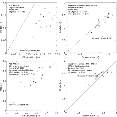
Fig. 7.Comparison between modelled and observed AOD (440 nm) and ˚Angstr¨om parameter (440–870 nm) at AERONET stations. Above:
Fig. 8. Graphical overview of the comparison between modelled and observed AOD (440 nm) and ˚Angstr¨om parameter (440–870 nm) at AERONET stations. The island in the upper box is Svalbard (Norway).
Fig. 9.Comparison between modelled and observed AOD per month. Valid data of all AERONET stations are averaged.
the free atmosphere, 75% of the nitrogen oxides is removed chemically and 25% is exported.
3.4 Optical analysis
In Table 5, Fig. 7 (upper panels) and Fig. 8, we compare the calculated optical data with AERONET observations. We clearly underestimeate AOD systematically, though the tem-poral variability is captured adequately by the model. Gener-ally, the AOD in summer is much higher than in winter, and the relative underprediction by TM5 is less in summer and early autumn (factor less than two) than in other months with a factor often above two (see Fig. 9). Also note that more data points are available in summer than in winter.
As the AOD is severely underestimated, we can conclude that besides the small underestimation of the PM10 surface
Fig. 10. Time series of modelled and observed AOD (440 nm) for Dunkerque (left) and Minsk (right). Upper panels: Only climatologic GFED emissions. Lower panels: New simulation with FAS-SILAM emissions. Both simulations use the regular wet-deposition rates.
affect surface PM10concentrations rather than AOD. We will
show in Sect. 3.5.2 that the severe underestimation of the AOD in eastern Europe is largely explained by inadequate biomass burning emission used by the model. The underes-timation of the AOD may also be related to too high wet-deposition rates (Chin et al., 2000). Wet wet-deposition is a dom-inant term in the budget (Tables 3 and 4) and we will address this further in Sect. 3.5.1.
At those stations that are located within or near major source regions of black carbon, part of the underestimation of AOD values may derive from biases introduced by the homogeneous sphere approximation, which is employed in Mie computations. For instance, externally mixed black car-bon aggregates absorb twice as much radiation in the atmo-sphere as volume-equivalent homogeneous atmo-spheres (Kahnert, 2010a,b). Model computations that account for inhomoge-neous mixing of BC with soluble aerosol components pre-dict absorption cross sections that are a factor of 1.5 higher than those computed with a homogeneous mixture approxi-mation (Bond et al., 2006). Such morphological effects are
neglected in our effective medium and Mie computations and may contribute to the AOD bias.
There is a reasonable temporal correlations between ob-served and modelled ˚Angstr¨om parameter (Table 5). The yearly averages agree very well. Also, the spatial variabil-ity among station is represented very well. There is one ex-ception (Hornsund, Svalbard), which is due to the low AOD values there, making the ˚Angstr¨om parameter very sensitive to errors.
3.5 Uncertainty analysis
In this section, we will investigate the uncertainties related to two key processes: wet removal and emission strengths. With sensitivity simulations we explore possible explana-tions for the underestimation of the AOD.
3.5.1 Wet deposition
Table 5.Comparison between modelled and observed optical parameters. Listed are temporal correlations and averages of time series of the AOD 440 nm and the ˚Angstr¨om parameter 440–870 nm at 18 European AERONET stations.
AOD 440 nm Angstr¨om 440–870 nm˚
Station name temp.r model obs. temp.r model obs. # points
Belsk 0.37 0.162 0.296 0.47 1.577 1.524 992
Cabauw 0.58 0.138 0.323 0.71 1.332 1.173 515
Chilbolton 0.68 0.103 0.235 0.58 1.102 1.156 746 Dunkerque 0.59 0.105 0.277 0.52 1.221 1.202 686 El Arenosillo 0.78 0.175 0.268 0.70 0.813 0.915 62 Forth Crete 0.58 0.187 0.233 0.72 1.092 1.108 1787
Granada 0.61 0.117 0.210 0.39 0.997 1.057 1733
Hamburg 0.38 0.102 0.246 0.27 1.410 1.481 843
Hornsund 0.51 0.015 0.135 0.45 0.657 1.298 265
Ispra 0.49 0.107 0.307 0.30 1.403 1.520 1280
Karlsruhe 0.60 0.149 0.334 0.57 1.435 1.394 623 La Fauga 0.61 0.117 0.205 0.55 1.222 1.403 1275
Messina 0.40 0.127 0.226 0.47 1.063 1.198 784
Minsk 0.06 0.086 0.303 0.61 1.429 1.505 669
Moldova 0.38 0.144 0.257 0.53 1.504 1.668 1302
Moscow MSU MO 0.29 0.132 0.320 0.48 1.555 1.528 772 Rome Tor Vergata 0.63 0.154 0.238 0.60 1.317 1.326 1679
SMHI 0.66 0.062 0.184 0.60 1.270 1.160 700
therefore explain why the AOD is underestimated while the surface concentrations look reasonable. We performed three additional simulations for May, June and July 2006 with all in-cloud scavenging rates (both for stratiform and convec-tive precipitation) scaled down to respecconvec-tively 50%, 10% and 0%. It appeared that halving (50%) the in-cloud scaveng-ing hardly made any difference in the simulated AOD values (about 10% higher AOD after spin-up). This clearly indicates the high efficiency of wet deposition in TM5. As expected, completely ignoring it (0%) resulted in unrealistically high values for the AOD (factor 6 after three months and ever rising). We will analyse the 10% wet-removal simulation, which showed a clear improvement, for the analysis period June and July 2006.
Figure 7 (lower panels) shows that in the 10% simulation, the large underestimation of the AOD has been turned into a slight overestimation. The ˚Angstr¨om parameter is still rep-resented quite well, which indicates that the aerosol size dis-tribution is little affected. Although the modelled AOD and
˚
Angstr¨om parameter now agree in Hornsund, the temporal correlation between model and observations at that station remains very poor (not shown). In general, the temporal cor-relations remain roughly similar (not shown).
We also investigated the changes in surface concentrations that result from a reduction of in-cloud scavenging to 10%. Sulphate and sea salt concentrations rise significantly (about 50%), while other compounds change only very little. From Fig. 3, it is clear that we already overestimate sea salt by 50%. Also the agreement of surface concentrations of
sul-phate, good in the unperturbed simulation as shown in Fig. 3, slightly deteriorates by reducing the wet-removal rates.
It appears that a scaling factor of 10% on the wet-deposition rates results in slightly too high surface concentra-tions and AOD values. For AOD, we expect a slight underes-timation because of non-implemented emissions of biogenic volatile compounds and resuspension. The signal of the sur-face concentrations also indicates that with a 10% scaling of the in-cloud scavenging, the wet removal is underestimated. The aerosol budget changes mainly in the free troposphere. Based on an analysis of the months June and July, we esti-mate that the wet-deposition flux is roughly halved in favour of the net export.
We refrain from a further tuning of the wet deposition here, because a sound parameterisation should be based on the physical and numerical considerations (e.g. grid-size de-pendency) that are associated with both stratiform and con-vective wet removal. We have shown, however, that a poor representation of wet deposition may be a major cause of the general underestimation of the AOD and may have masked other model deficiencies.
3.5.2 Forest fires
emissions tend to exhibit large variability between the years and between the seasons in a year (van der Werf et al., 2006). An extreme case occurred in spring 2006, when there were strong forest fires in western Russia (Sofiev et al., 2009; Saarikoski et al., 2007). These events take place every spring, but in 2006 they were particularly strong. Apart from that, the last week of April and the first week of May, the mean wind direction in eastern Europe (20◦E–30◦E) was easterly, which coincides with the fires. This transported the smoke towards Europe, so that it was recorded in the time series of the AOD in eastern European stations.
Figure 10 (upper two graphs) shows a comparison between modelled and observed AOD for Dunkerque and Minsk, in which we can see that Minsk exhibits a clearly separate pop-ulation of points that belong to the period of the forest fires. For Dunkerque, the points of this period are more mixed with the rest of the dataset. The high observed AOD values dur-ing the event were not reproduced by the model. Because easterly circulation is associated with fair weather, the possi-ble too high wet-deposition rates in the model is not likely to play a significant role.
To reproduce the high AOD values at the eastern Euro-pean stations, we repeated the simulation with the EuroEuro-pean emission data from the Fire Assimilation System (FAS) that was used in combination with the dispersion model SILAM (Sofiev et al., 2009). The FAS-SILAM PM2.5 emissions
in the area specified below are 4.3 Tg for the considered monthly period, while the climatologic GFED emissions in that area were only 8.7 Gg per month (500 times less). More-over, the GFED emissions are temporally spread over the entire months, while FAS reported them with daily resolu-tion. As the majority of the emissions occurred during the days with easterly winds, it was evidently important to apply a daily time resolution of emissions to capture the specific transport conditions during the event.
The FAS-SILAM emission data consist of daily 2D fields of PM2.5emissions in Europe (11◦W–73◦E, 34◦N–80◦N).
We assumed that 10% of this PM2.5is black carbon and 90%
is organic matter, which is a rough estimation based on ob-servations in Saarikoski et al. (2007). This assumption may influence the results as the optical properties of black carbon and organic matter are different. Also, the injection height of these emissions can be important (Chen et al., 2009). We as-sumed the following distribution injection heights following Dentener et al. (2006): 20% between surface and 100 m, 20% between 100 m and 500 m, 20% between 500 m and 1 km and 40% between 1 km and 2 km. We performed a simulation, re-placing the original climatologic emissions from 15 April to 14 May.
Figure 10 (lower two graphs) show the results for the two AERONET stations. There is a drastic improvement for Minsk, which indicates that this event is caught by the model including these emissions. There is also a small improve-ment in the results for Dunkerque as well, which means that Dunkerque is affected by these emissions through long range
transport. The improvement in the model results clearly il-lustrates that episodic fire events at the eastern edge of Eu-rope in combination with certain transport patterns may have a significant impact throughout the European domain.
4 Conclusions
Size-resolved aerosol simulations with the TM5 model cou-pled to the M7 module have been conducted for the year 2006 with a focus on the European domain (34◦N–62◦N, 12◦W– 36◦E). The main conclusions can be summarised as follows:
– Comparison of the simulated aerosol distribution with surface observations over Europe shows a reasonably good agreement with spatial correlations of simulated PM mass of 0.75. As expected, spatial correlations are lowest (r= 0.64) and biases are highest for PM10,
pos-sibly due to neglected resuspension of aerosols. Total ammonium (r= 0.61) is overestimated in the high con-centration range, due to the overestimation of NH3 in
emission regions.
– A three-dimensional budget analysis is carried out to en-able model intercomparison and assessement of impor-tant uncertainties. From our budget, we can conclude that Europe is a net exporter of anthropogenic aerosols, and an importer of natural aerosols (sea salt and min-eral dust). For instance, it is calculated that about half of the emitted anthropogenic carbonaceous aerosols are exported from Europe. Dust is the only aerosol compo-nent that exhibits a negative vertical flux over the Euro-pean domain. Notable is that the export rate of gaseous pollutants (e.g. nitrogen oxides) is considerably lower than for anthropogenic aerosols because of dry deposi-tion.
– A comparison to AERONET AOD measurements shows a serious underestimation of the modelled AOD values. We showed that a significant downscaling of the wet-removal rates in the model is required to bring the model closer to the observations. This, however, significantly raises the modelled surface sulphate and sea salt concentrations, while other components are lit-tle affected. The modelled ˚Angstr¨om parameter is little affected, which indicates that the aerosol size distribu-tion remains roughly the same.
Based on this study, future model developments will tar-get at improving the aerosol wet-deposition parameterisa-tion in the TM5 model and the aerosol emission inventories. TM5 employs multiple resolutions at the same time, which calls for a fundamental approach of resolution-dependent processes like the wet removal of aerosols. Fire emissions, but also the emissions of aerosol precursors such as NH3
ex-hibit day-to-day variability and diurnal emission patterns that should be taken into account to enable a sound comparison to observations. Finally, it is recommended to continue inter-model (Wilson et al., 2001; Bauer et al., 2008; de Meij et al., 2006) comparisons based on budget analysis as presented in this paper or similar techniques (Textor et al., 2006).
Acknowledgements. This work benefited from measurements
by the Programme for Monitoring and Evaluation of the Long-range Transmission of Air Pollutants in Europe (EMEP) and the Aerosol Robotic Network (AERONET). We thank the principal investigators of these networks and their staff for establishing and maintaining the sites used in this investigation. This research received financial support from the BOP (Policy supporting programme for particulate matter). We would like to thank the NCF (Foundation of national computer facilities) for providing the ability to run TM5 on the supercomputer Huygens. We would like to thank Olivier Boucher for programming Mie scattering calculations for aerosol distributions. M. Kahnert was supported by the Swedish Research Council under contract number 80438701.
Edited by: Y. Balkanski
References
Anderson, T. L., Charlson, R. J., Schwartz, S. E., Knutti, R., Boucher, O., Rodhe, H., and Heintzenberg, J.: Climate forc-ing by aerosols – a hazy picture, Science, 300, 1103–1104, doi: 10.1126/science.1084777, 2003.
Andres, R. J. and Kasgnoc, A. D.: A time-averaged inventory of subaerial volcanic sulfur emissions, J. Geophys. Res., 103, 25251–25261, doi:10.1029/98JD02091, 1998.
˚
Angstr¨om, A. K.: On the atmospheric transmission of sun radiation and on the dust in the air, Geogr. Ann., 11, 156–166, 1929. Balkanski, Y. J., Jacob, D. J., Gardner, G. M., Graustein, W. C.,
and Turekian, K. K.: Transport and residence times of tropo-spheric aerosols inferred from a global trhee-dimensional sim-ulation of 210Pb., J. Geophys. Res., 98, 20573–20586, doi: 10.1029/93JD2456, 1993.
Barber, P. W. and Hill, S. C.: Light scattering by particles: Com-putational Methods, Advanced series in applied physics, World Scientific, 2, 261 pp., 1990.
Bauer, S. E., Wright, D. L., Koch, D., Lewis, E. R., McGraw, R., Chang, L.-S., Schwartz, S. E., and Ruedy, R.: MATRIX (Multiconfiguration Aerosol TRacker of mIXing state): an aerosol microphysical module for global atmospheric models, Atmos. Chem. Phys., 8, 6003–6035, doi:10.5194/acp-8-6003-2008, 2008.
Berkvens, P. J. F., Botchev, M. A., Lioen, W. M., and Verwer, J. G.: A Zooming Technique for Wind Transport of Air
Pollu-tion, in: Finite volumes for complex applications: problems and perspectives: internation symposium, Duisburg, Germany, 499– 506, 1999.
Bond, T. C., Streets, D. G., Yarber, K. F., Nelson, S. M., Woo, J.-H., and Klimont, Z.: A technology-based global inventory of black and organic carbon emissions from combustion, J. Geo-phys. Res., 109, D14203, doi:10.1029/2003JD003697, 2004. Bond, T. C., Habib, G., and Bergstrom, R. W.: Limitations in the
enhancement of visible light absorption due to mixing state, J. Geophys. Res., 111, D20211, doi:10.1029/2006JD007315, 2006. Boucher, O.: On Aerosol Direct Shortwave Forcing and the Henyey-Greenstein Phase Function, J. Atmos. Sci., 55, 128– 134, doi:10.1175/1520-0469(1998)055h0128:OADSFAi2.0.CO; 2, 1997.
Bouwman, A. F., Lee, D. S., Asman, W. A. H., Dentener, F. J., van der Hoek, K. W., and Olivier, J. G. J.: A global high-resolution emission inventory for ammonia, Global Biogeochem. Cy., 11(4), 561–587, doi:10.1029/97GB02266, 1997.
Bregman, B., Segers, A., Krol, M., Meijer, E., and van Velthoven, P.: On the use of mass-conserving wind fields in chemistry-transport models, Atmos. Chem. Phys., 3, 447–457, doi:10.5194/acp-3-447-2003, 2003.
Bruggeman, D. A. G.: Berechnung verscheidener physikalis-cher Konstanten von heterogenen Substanzen, 1. Dielek-trizit¨atskonstanten und Leitf¨ahigkeiten der Mischk¨orper aus isotropen Substanzen, Ann. Phys., 416, 636–664, doi:10.1002/ andp.19354160802, 1935.
Brunekreef, B. and Holgate, S. T.: Air pollution and health, Lancet, 360, 1233–1242, doi:10.1016/S0140-6736(02)11274-8, 2002. Buijsman, E., Maas, H. F. M., and Asman, W. A. H.: Anthropogenic
NH3emissions in Europe, Atmos. Environ., 21, 1009–1022, doi:
10.1016/0004-6981(87)90230-7, 1987.
Chen, Y., Li, Q., Randerson, J. T., Lyons, E. A., Kahn, R. A., Nel-son, D. L., and Diner, D. J.: The sensitivity of CO and aerosol transport to the temporal and vertical distribution of North Amer-ican boreal fire emissions, Atmos. Chem. Phys., 9, 6559–6580, doi:10.5194/acp-9-6559-2009, 2009.
Cheng, Y. H. and Tsai, C. J.: Evaporation loss of ammonium nitrate particles during filter sampling, J. Aerosol Sci., 28, 1553–1567, doi:10.1016/S0021-8502(97)00033-5, 1997.
Chin, M., Rood, R. B., Lin, S.-J., M¨uller, J.-F., and Thompson, A. M.: Atmospheric sulfur cycle simulated in the global model GOCART: Model description and global properties, J. Geophys. Res., 105, 24671–24687, 2000.
Cofala, J., Amann, M., and Mechler, R.: Scenarios of world an-thropogenic emissions of air pollutants and methane up to 2030, Tech. rep., International Institute for Applied System Analysis (IIASA), Laxenburg, Austria, online available at: http://www. iiasa.ac.at/rains/global emiss/global emiss.html, (last access: 9-7-2009), 2005.
Dana, M. T. and Hales, J. M.: Statistical aspects of the washout of polydisperse aerosols, Atmos. Environ., 10, 45–50, doi:10.1016/ 0004-6981(76)90258, 1976.
Dentener, F. and Crutzen, P. J.: A Three-dimensional Model of the global ammonia cycle, J. Atmos. Chem., 19, 331–369, doi:10. 1007/FG00694492, 1994.
G. R., and Wilson, J.: Emissions of primary aerosol and pre-cursor gases in the years 2000 and 1750 prescribed data-sets for AeroCom, Atmos. Chem. Phys., 6, 4321–4344, doi:10.5194/acp-6-4321-2006, 2006.
Dockery, D., Pope, C. A., Xu, X., Spengler, J. D., Ware, J. H., Fay, M. E., Ferris, B. G., and Speizer, F. E.: An association between air pollution and mortality in siz US cities, New Engl. J. Med., 329, 1753–1759, doi:10.1056/NEJM199312093292401, 1993. European Monitoring and Evaluation Programma: Hjellbrekke,
A.-G., and Fjæraa, A. M.: Data report 2006: Acidifying and eutro-phying compounds and particulate matter, Tech. rep., 2008. Ganzeveld, L., Lelieveld, J., and Roelofs, G.-J.: A dry
deposi-tion parameterizadeposi-tion for sulfur oxides in a chemistry and gen-eral circulation model, J. Geophys. Res., 103, 5679–5694, doi: 10.1029/97JD03077, 1998.
von Glasgow, R.: Pollution meets sea salt, Nat. Geosci., 1, 292–293, doi:10.1038/ngeo192, 2008.
Gong, S. L.: A parameterization of sea-salt aerosol source function for sub- and super-micron particles, Global Biogeochem. Cy., 17, 1097, doi:10.1029/2003GB002079, 2003.
Guelle, W., Balkanski, Y. J., Schultz, M., Dulac, F., and Monfray, P.: Wet deposition in a global size-dependent aerosol transport model 1. Comparison of a 1 year210Pb simulation with ground measurements, J. Geophys. Res., 103, 28875–28891, 1998. Halmer, M. M., Schmincke, H.-U., and Graf, H.-F.: The annual
volcanic gas input into the atmosphere, in particular into the stratosphere: a global data set for the past 100 years, J. Vol-canol. Geoth. Res., 115, 511–528, doi:10.1016/S0377-0273(01) 00318-3, 2002.
Haywood, J. and Boucher, O.: Estimates of the direct and indirect radiative forcings due to tropospheric aerosols: a review, Rev. Geophys., 38, 513–543, 2000.
Hess, M., Koepke, P., and Schult, I.: Optical Properties of Aerosols and Clouds: The Software Package OPAC, B. Am. Meteo-rol. Soc., 79, 831–844, doi:10.1175/1520-0477(1998)079h0831: OPOAACi2.0.CO;2, 1998.
Hicks, B. B., Wesely, M. L., Coulter, R. L., Hart, R. L., Durham, J. L., Speer, R., and Stedman, D. H.: An experimental study of sulfur and NOxfluxes over grassland, Bound. Lay. Meteorol., 34,
103–121, 1986.
Hoek, G., Brunekreef, B., Goldbohm, S., Fischer, P., and van den Brandt, A.: Association between mortality and indicators of traffic-related air pollution in the Netherlands: a cohort study, Lancet, 360, 1203–1209, doi:10.1016/S0140-6736(02)11280-3, 2002.
Holben, B. N., Tenr´e, D., Smirnov, A., Eck, T. F., Slutsker, I., Abuhassan, N., Newcomb, W. W., Schafer, J. S., Chatenet, B., Lavenu, F., Kaufman, Y. J., Vande Castle, J., Setzer, A., Markham, B., Clark, D., Frouin, R., Halthore, R., Karneli, A., O’Neill, N. T., Pietras, C., Pinker, R. T., Voss, K., and Zibordi, G.: An emerging ground-based aerosol climatology: Aerosol optical depth from AERONET, J. Geophys. Res., 106, 12067– 12097, 2001.
Holtslag, A. A. M. and Boville, B. A.: Local versus nonlocal boundary-layer diffusion in a global climate model, J. Climate, 6, 1825–1842, doi:10.1175/1520-0442(1993)006h1825:LVNBLDi 2.0.CO;2, 1993.
Houweling, S., Dentener, F., and Lelieveld, J.: The impact of non-methane hydrocarbon compounds on tropospheric
photochem-istry, J. Geophys. Res., 103, 10673–10696, 1998.
Intergovernmental Panel on Climate Change: edited by: Nakicen-ovic, N., Akamo, J., Davis, G., de Vries, B., Fenhann, J., Gaffin, S., Gregory, K., Gr¨ubler, A., Jung, T. Y., Kram, T., La Rovere, E. L., Michaelis, L., Mori, S., Morita, T., Pepper, W., Pitcher, H., Price, L., Riaki, K., Roehrl, A., Rogner, H.-H., Sankovski, A., Schlesinger, M., Shukla, P., Smith, S., Swart, R., van Rooijen, S., Victor, N., and Dadi, Z.: Special report on Emissions Scenar-ios, 2000.
Intergovernmental Panel on Climate Change, edited by: Solomon, S., Qin, D., Manning, M., Chen, Z., Marquis, M., Averyt, K. B., Tignor, M., and Miller, H. L.: Climate change 2007: The physi-cal Science Basis, IPCC Fourth Assassement report (AR4), 2007. Kahnert, M.: Modelling the optical and radiative properties of freshly emitted light absorbing carbon within an atmospheric chemical transport model, Atmos. Chem. Phys., 10, 1403–1416, doi:10.5194/acp-10-1403-2010, 2010a.
Kahnert, M.: Numerically exact computations of the optical properties of light absorbing carbon aggregates for wavelength of 200 nm–12.2 µm, Atmos. Chem. Phys., 10, 8319–8329, doi:10.5194/acp-10-8319-2010, 2010b.
Kanakidou, M.: Aerosols in Global Models – Focus on Europe, in: Regional Climate Variability and its Impacts in The Mediter-ranean Area, chap. 4, Springer, The Netherlands, 143–154, 2007. Kanakidou, M., Seinfeld, J. H., Pandis, S. N., Barnes, I., Dentener, F. J., Facchini, M. C., Van Dingenen, R., Ervens, B., Nenes, A., Nielsen, C. J., Swietlicki, E., Putaud, J. P., Balkanski, Y., Fuzzi, S., Horth, J., Moortgat, G. K., Winterhalter, R., Myhre, C. E. L., Tsigaridis, K., Vignati, E., Stephanou, E. G., and Wilson, J.: Organic aerosol and global climate modelling: a review, At-mos. Chem. Phys., 5, 1053–1123, doi:10.5194/acp-5-1053-2005, 2005.
Kaufman, Y. J., Tenr´e, D., and Boucher, O.: A satellite view of aerosols in the climate system, Nature, 419, 215–223, 2002. Kerkweg, A., Buchholz, J., Ganzeveld, L., Pozzer, A., Tost, H.,
and J¨ockel, P.: Technical Note: An implementation of the dry removal processes DRY DEPosition and SEDImentation in the Modular Earth Submodel System (MESSy), Atmos. Chem. Phys., 6, 4617–4632, doi:10.5194/acp-6-4617-2006, 2006. Kinne, S., Lohmann, U., Feichter, J., Schultz, M., Timmreck, C.,
Ghan, S., Easter, R., Chin, M., Ginoux, P., Takemura, T., Tegen, I., Koch, D., Herzog, M., Penner, J., Pitari, G., Holben, B., Eck, T., Smirnov, A., Dubovik, O., Slutsker, I., Tanre, D., Tarnes, O., Mishchenko, M., Geogdzhayev, I., Chu, D. A., and Kaufman, Y.: Monthly averages of aerosol properties: A global compari-son among models, satellite data and AERONET ground data, J. Geophys. Res., 108, 2634, doi:10.1029/2001JD001253, 2003. Korhonen, H., Carslaw, K. S., Spracklen, D. V., Ridley, D. A., and
Str¨om, J.:A global model study of processes controlling aerosol size distributions in the Arctic spring and summer, J. Geophys. Res., 113, D08211, doi:10.1029/2007JD009114, 2008.
Krol, M., Houweling, S., Bregman, B., van den Broek, M., Segers, A., van Velthoven, P., Peters, W., Dentener, F., and Bergamaschi, P.: The two-way nested global chemistry-transport zoom model TM5: algorithm and applications, Atmos. Chem. Phys., 5, 417– 432, doi:10.5194/acp-5-417-2005, 2005.