Universidade Nova de Lisboa Faculdade de Ciências e Tecnologia Departamento de Informática An Implementation of Dynamic Fully Compressed Suffix Trees

(1)

Universidade Nova de Lisboa

Faculdade de Ciências e Tecnologia

Departamento de Informática

An Implementation of Dynamic Fully Compressed

Suﬃx Trees

Miguel Filipe da Silva Figueiredo

Dissertação apresentada na

Faculdade de Ciências e Tecnologia da Universidade Nova de Lisboa

para obtenção do grau de Mestre em Engenharia Informática

Orientador: Prof. Dr. Luís Russo

(2)

Resumo

Esta dissertação estuda e implementa uma árvore de sufixos dinâmica e com-primida. As árvores de sufixos são estruturas de dados importantes no estudo de cadeias de caracteres e têm soluções óptimas para uma vasta gama de problemas. Organizações com muitos recursos, como companhias da biomedicina, utilizam computadores poderosos para indexar grandes volumes de dados e correr algorit-mos baseados nesta estrutura. Contudo, para serem acessíveis a um publico mais vasto as árvores de sufixos precisam de ser mais pequenas e práticas. Até recen-temente ainda ocupavam muito espaço, uma árvore de sufixos dos 700 megabytes do genoma humano ocupava 40 gigabytes de memória.

A árvore de suﬁxos comprimida reduziu este espaço. A árvore de suﬁxos estática e comprimida requer ainda menos espaço, de facto requer espaço comprimido opti-mal. Contudo, como é estática não é adequada a ambientes dinâmicos. Chan et al. [3] descreveram a primeira árvore dinâmica comprimida, todavia o espaço usado para um texto de tamanho n_é O₍n_logσ_{) bits, o que está longe das propostas}

es-táticas que utilizam espaço perto da entropia do texto. O objectivo é implementar a recente proposta por Russo, Arlindo e Navarro[22] que deﬁne a árvore de suﬁxos dinâmica e completamente cumprimida e utiliza apenas nH_k₊O₍n_logσ_{) bits de}

(3)

Abstract

This dissertation studies and implements a dynamic fully compressed suffix tree. Suffix trees are important algorithms in stringology and provide optimal solutions for myriads of problems. Suffix trees are used, in bioinformatics to index large volumes of data. For most aplications suffix trees need to be efficient in size and funcionality. Until recently they were very large, suffix trees for the 700 megabyte human genome spawn 40 gigabytes of data.

The compressed suffix tree requires less space and the recent static fully compressed suffix tree requires even less space, in fact it requires optimal compressed space. However since it is static it is not suitable for dynamic environments. Chan et. al.[3] proposed the first dynamic compressed suffix tree however the space used for a text of size n _is O₍n_logσ_{)bits which is far from the new static solutions. Our}

goal is to implement a recent proposal by Russo, Arlindo and Navarro[22] that deﬁnes a dynamic fully compressed suﬃx tree and uses onlynH₀₊O₍n_logσ_{) bits}

(4)

List of Figures

2.1 Suﬃx tree for the text "mississippi". . . 15

2.2 A sub-tree of the suﬃx tree for string "mississippi". . . 17

2.3 Suﬃx array of the text "mississippi". . . 18

2.4 Rank of of size four bitmaps with two "1"s. . . 23

2.5 Static structure for rank and select with superblocks, blocks and bitmaps. . . 24

2.6 Bitcoding for the text "mississippi". . . 25

2.7 The wavelet tree for the text "mississippi". . . 25

2.8 Matrix M of the Burrows Wheeler Transform. . . 28

2.9 Matrix M of the Burrows Wheeler Transform with operations computed during a backward search. . . 30

2.10 Parentheses representation of the suﬃx tree for "mississippi". . 31

2.11 Sampled suﬃx tree with suﬃx links. . . 34

2.12 ALCP table and the operations required to performSLink(3,6). 37 2.13 A binary tree with p and r values at the nodes and bitmaps at the leaves. . . 40

2.14 Matching parentheses example. . . 45

2.15 Computing opened values for blocks. . . 46

2.16 Computing closed values for blocks. . . 46

2.17 Computing closed and opened values for several blocks. . . 47

2.18 Computing LCA of two nodes. . . 48

2.19 Reversed tree of the suﬃx tree for "mississippi", also the sam-pled suﬃx tree of "mississippi". . . 52

(7)

3.2 The suﬃx tree structure and the DFCST structure. . . 58

3.3 A sampling creates a sampled node with the wrong string depth. 59 3.4 Leaf insertion creating a sampling error. . . 60

3.5 Weiner node computation. . . 61

3.6 Computation of LCA. . . 62

3.7 Child computation with a binary search. . . 64

3.8 The wavelet tree data structure using a binary tree. . . 65

3.9 The wavelet tree data structure using a heap. . . 66

3.10 Compact wavelet tree data structure with a binary tree. . . . 67

3.11 Sorted access implementation for the wavelet tree. . . 68

3.12 Compact wavelet tree data structure with a heap. . . 68

3.13 The bit tree buﬀering. . . 72

3.14 The redistribution operation of a critical bitmap block. . . 74

3.15 Compacting the parentheses tree. . . 77

4.1 The space ratio for bit trees with arity 10, 100 and 1000. . . . 82

4.2 The build time for bit trees with arity 10, 100 and 1000. . . . 83

4.3 The time used to complete a batch of operations for bit trees with arity 10, 100 and 1000. . . 83

4.4 The space ration for the RB bit tree and the B+ bit tree. . . . 84

4.5 The build time statistic for the RB bit tree and the B+ bit tree. 85 4.6 The time statistic for completion of a batch of operations with the RB bit tree and the B+ bit tree. . . 85

4.7 Bit trees compared over three criteria. . . 86

4.8 Comparing the bit tree normal build and the alternated dele-tion build. . . 88

4.9 Comparing the space used per node of normal trees and paren-theses trees. . . 89

4.10 Comparing wavelet trees space. . . 91

4.11 Comparing wavelet trees speed. . . 91

4.12 DFCST space use results. . . 93

(8)

List of Tables

1.1 The table shows notations used. . . 12

1.2 The table shows notations used. . . 13

2.1 The table shows time and space complexities for Sadakane static CST and Russo et al. FCST. . . 36

2.2 The table shows time and space complexities for Chan et al. dynamic CST and Russo et al. dynamic FCST. . . 55

4.1 Test machine descriptions. . . 80

4.2 DFCST and FCST operations time. . . 94

(9)

Chapter 1 Introduction

1.1 General Introduction

The organization of data and its retrieval is a fundamental pillar for the sci-entiﬁc development. In the 20Th century the science of information retrieval has matured, its early days may be traced to the development of tabulating machines by Hollerith in 1890. From the 1960s through to the 1990s several techniques were developed showing that information retrieval on small docu-ments was feasible using computers. The Text Retrieval Conference, part of the TIPSTER program, was sponsored by the US government and focused on the importance of eﬃcient algorithms for information retrieval of large texts. The TIPSTER created a infrastructure for the evaluation of text retrieval techniques on large texts, furthermore when web search engines were intro-duced in 1993 the area of data retrieval continued to prosper. Search engines relish on information retrieval and are strong investors in such technology.

(10)

advantage of the latest developments on databases, algorithms, computa-tional and statistical techniques to study problems that are otherwise too complex in today’s computers. Exact matching is a sub-task used in sev-eral problems dealing with DNA, RNA, processed patterns or amino acid rings. As such developments in this area provide beneﬁts to a wide range of bio-informatics applications.

1.2 Problem Description and Context

Searching for genes in DNA is a common problem in bio-informatics. Find-ing a specific gene sequence within the human genome is a big task and feasible only with the most advanced computers. The results are otherwise prohibitively time consuming. Several problems arise when searching for damaged or mutated genes and the algorithms used can consume a lot of time to process these queries. Problems related to finding a specific string within other string are referred to as exact string matching. Finding a string with some form of errors is a inexact string matching. String matching is not limited to DNA, in fact these problems are of great use for other scien-tific areas, for example it is essential for large Internet search engines, since information grows exponentially yearly.

(11)

which yields an extremely large suffix tree. Suffix trees have problematic space requirements. Uncompressed suffix trees can use from 10 to 20 times the size of the original text. A simple implementation of a suffix tree for the human genome consumes 40 gigabytes, as a consequence this tree requires secondary memory. In this case operations will slow down so extremely that it renders the structure useless[10]. Hence several techniques were created to save space and represent suffix trees in a more practical size.

Suffix arrays were developed by Eugene Myers and Udi Manber and in parallel by Baeza Yates and Garton Gonet. These data structures are based on suffix trees but can be stored in much less space[16]. They consists in a array with the starting positions of all suffixes in the the text arranged by lexicographical order. Suffix arrays are used to locate suffixes within a string and can be extended to determine the longest common prefixes of any two suffixes, however they can support only a limited subset of the operations provided by the suffix tree, still by adding extra structures it is possible to simulate a suffix tree algorithm[2].

Another classical attempt to reduce space is the directed acyclic graph. It represents strings and supports constant time search for suﬃxes. During construction isomorphic sub trees are detected and it generates a acyclic directed graph instead of a tree.

The main achievement and difference between tries and dags is the elimina-tion of suffix redundancy in the trie. Both tries and dags eliminate prefix redundancy but only dags eliminate both prefix and suffix redundancy.

(12)

Suffix trees solve the pattern matching problem in the same worst case linear timeO(n+α_×m). However because the preprocessed string is the text, and with a larger α, time is linear on the size of the patterns which normally is much smaller. When there are several patterns to search the speed advan-tage of reusing the preprocessed suffix tree is obvious. The linear algorithms will always spend time preprocessing the patterns and running the text in linear time while suffix trees only need to preprocess the text once and run the patterns in linear time.

The Aho Corasick achieves a time similar to suffix trees as it matches a set of patterns with a text. However the largest speed advantage of suffix trees over classical linear algorithms appears in problems that are more complex than exact string matching. For example the longest common substring problem can be solved in linear algorithms by suffix trees and there are no other known linear time algorithms. The linear algorithms will always search for a exact string at every run, however the suffix tree has a structure that allows it to find all substrings in the same run with little time cost.

Suffix arrays can be enhanced to support all functions that suffix trees do with similar times and additional structures. Since suffix trees solve different classes of problems thanks to some properties(suffix links, bottom up and top down traversal) the enhanced suffix arrays add structures that simulate all those properties. Though using less space than conventional suffix trees the overall space cost is high.

(13)

space result for a compressed suffix tree. It discards the space used by the compressed suffix tree of Sadakane and achieves a smaller space than the entropy bounded compressed suffix tree[24]. It achieves a compressed space suffix tree for the first time, the times of most operations are logarithmic or near logarithmic. The implementation of this structure recently presented by Russo has proven this result. This dissertation compares results with the implementation by Russo.

The recent space reduction by Russo, Arlindo and Navarro takes static suffix trees down to compressed space[12]. Although this is a important result, this suffix tree as well as other implementations of similar sizes, is statical. The lack of dynamic insertions and deletions, makes these implementations unsuited for problems within a dynamic environment. This has a significant impact in the space that is used at build time. During this initial fase the suffix tree needs space that is discarded once construction is complete.

1.3 Proposed Solution

A solution proposed by Russo, Arlindo and Navarro[22] solves both the dy-namic suffix tree problem and the construction space problem. There is a cost of adding dynamic capabilitie to the fully compressed suffix tree, which is a logarithmic slow down on the operations. This dissertation proposes to implement this dynamic fully compressed suffix tree.

1.4 Main Achievements

(14)

compressed suﬃx within reasonable space not overcoming the ﬁnal space. We obtain the following results:

• An implementation of a dynamic suﬃx tree.

• A small dynamic suﬃx tree, not larger than twice the text.

(15)

1.5 Simbols and Notations

Table 1.1: The table shows notations used.

Notation Deﬁnition

n size of a text

m size of a pattern

α size of a text

δ the sampling

σ the size of a alphabet

T a suﬃx tree

T−1 _{the reversed suﬃx tree}

i a index position

v a node

SLink(v) the suﬃx link of node v SDep(v) the string depth of node v T Dep(v) the tree depth of nodev

LCA(v, v′₎ _{the lowest common ancestor of node} _v _and _v′ LET T ER(v, i) the i-th letter in the path label of v

P arent(v) computes the parent of node v

excess number of opened parentheses minus the number of

closed parentheses in a balanced sequence of paren-theses

minexcess(l, r) positionibetweenl andr such thatexcess(l, i) is the smallest in the range (l, r)

SA suﬃx array

(16)

Table 1.2: The table shows notations used.

Notation Deﬁnition

BWT Burrow Wheeler transform LF last to ﬁrst mapping

M matrix with the cyclic shifts of a text

L the last comumn in M

F ﬁrst column in matrix M

LCP computes the longest common preﬁx over a range of suﬃxes

ψ(v) psi link of nodev

s a string

c a caracter

Sj superblock number j

Bk block number k

Gc the table of class c

Cc computes the number of characters lexicographically

smaller thanc in the text

$ a caracter that does not exist in the text

opened unmatched opened parentheses over a balanced

se-quence of parentheses

closed unmatched closed parentheses over a balanced

se-quence of parentheses

I integers sequence

Occ(c, k) counts the number of occurrences of charactercbefore position k in column L

W einerLink(v, c) computes the weiner link of nodev using letter c

A a bitmap

Rankc(s, i) counts letters ’c’ in s up to positioni

Selectc(s, i) computes the index position of thei’Th occurrence in

s

(17)

Chapter 2 Related Work

2.1 Text Indexing

In section 2.1.1 we describe the suffix tree data structure which, like other full text indexes, is an important tool for substring searching problems. However suffix trees tend to be excessively large, ie 10 to 20 times the text size. Since suffix trees are very functional hence reducing their space requirements is crucial. In section 2.1.2 we describe suffix arrays, which are more space efficient full text indexes.

2.1.1 Suﬃx Tree

(18)

the suﬃx tree is not complicated although it is not trivial either.

A suffix tree for a text T of size n is a rooted directed tree with n leaves. Each leaf has a distinct value from 1 to n. All tree edges have a non empty label with a string. Every path from the root that ends on a leafidescribes a suffix starting ati. The concatenation of the labels down to the leaf describe the suffixes so finding a pattern is done with comparisons between the labels and the pattern. Every internal node except the root must have at least two children. No two children out of a node may start with the same letter.

Figure 2.1: Suffix tree for the text "mississippi". The values at the leaves are the initial positions of a suffix in the text. To the right the sub-tree containing leaves 3, 4, 6 and 7 is in a box. The suffix links of the internal nodes are shown with dotted arrows.

(19)

pattern matching contains all the occurrences of the pattern, each leaf of the sub-tree represents one occurrence. For the example with "ssi" there are two occurrences at position 5 and 2, which are respectively the suffixes "ssippi" and ssissippi". If the pattern was "kitty" the process fails to find a label in the suffix tree that matched the pattern and conclude that no occurrences exist.

The suffix link for a node v with path x.α is usually denoted as SLink(v). The suffix links are defined for nodes and exist from nodevtov′_{, path label of} v′ _is_α_{. In Figure 2.1 there are four suffix links represented as arrows between}

internal nodes. For example the node with path "issi" has a suffix link leading to the node with path "ssi". An important case is the suffix links on the leaves, they are defined as ψ and can be computed in the compressed suffix array which are explained in section 2.1.2. The weiner link is the opposite operation of suffix link as it points in the reverse direction. Likewise in this dissertation the LF mapping is referred as the reverse of ψ because it will only exist for the leaves.

Two important concepts areSDepandT Dep, they are resp string depth and tree depth of a node. For example in the suﬃx tree of "mississippi" the node with path "issi" has SDep 4 because that is the string size of the path. The

T Depof the same node is 2, because it is the second node from the root. The

LCA is the lowest common ancestor between two nodes. In the suﬃx tree of "mississippi" the LCA of the node with path "sissippi$" and the node node with path "ssi" is the node with path "s" which corresponds to the largest common preﬁx between the two strings. The operationLET T ER(v, i) refers to the i-th letter in the path label ofv. The operationLAQT(v, d), tree level

ancestor querie of node v and height d, returns the highest ancestor of node

v that has a tree depth smaller or equal tod. The LAQS(v, d) is similar but

(20)

Figure 2.2: A sub-tree of the suﬃx tree for string "mississippi". The LCAof nodes 3 and 5 is node 1. For nodes 2 and 1 the LCA is node 1. TheSDep

and T Dep of node 5 is resp 3 and 2. While SDep and T Dep for node 4 is resp 9 and 3.

2.1.2 Suﬃx Array

Suffix arrays were defined in 1990 by Manber & Myers[16]. It is a data struc-ture that contains the suffixes of the text that and occupies less space than a suffix tree. A suffix arrays for a text T, of sizen, is an arraySAof integers in the range 1 to n containing the start location of the lexicographically sorted suffixes of T. Every position in SA contains a suffix and SA[1] stores the lexically smallest suffix in T. The suffixes grow lexically at every consecutive position of SA[i] to SA[i+ 1].

(21)

the α occurrences it uses O(mlog n+α) time [13].

Figure 2.3: Suffix array of the text "mississippi". The figure shows the index positions (leftmost), theSAvalues(second column) and the list of suffixes. At the right and horizontally is the text "mississippi$" with the index positions.

A important operation that can be implemented with suffix arrays is the longest common prefix of a interval of suffixes, LCP. The longest common prefix of two suffixes in the tree is the common path the two suffixes share in the top down tree traversal. For example to determine the LCP of the suffix "ississippi" and the suffix "issippi", see Figure 2.1. Start at the root then follow the path with "i", then choose the path with "ssi", at this point the suffixes path diverge and the pattern "issi" is determined as the longest common prefix. Note that a node in the suffix tree corresponds to an interval in the suffix array, therefore finding the LCP of such an interval corresponds to computing the SDep of that node. The structure used in suffix arrays for this operation is the LCP table, it stores for each index the length of the LCP between the current index position and the previous position, i.e.

LCP[i] = Longest Common Preﬁx_{SA[i], SA[i₋1]_}.

(22)

and j. For example compute theSDep of the sub-tree in Figure 2.2. The vl

and vr are respectively 9 and 12, the smallest integer from index 9 to index

12 in the LCP table computing RM Q(vl+1, vr, LCP) = 1. Therefore the

SDep of the sub-tree is 1, the LCP of the suffix array index positions 9 to 12 is "s". In figure 2.3 the positions 9 through 12 correspond to suffixes 7, 4, 6 and 3, therefore the common prefix of the suffixes in this sub-tree is "s".

A form of compacting the suffix array was researched in 2000 by Mäkinen[14]. In parallel a concept for compression of a suffix array was found in 2000 by Grossi & Vitter[9]. These two ideas of compact and compressed suffix arrays represent notable advances towards space reduction. The compact suffix array uses the self repetitions in the SA to store it in less space. It was later proved by Mäkinen and Navarro[13] that the size of the compact suffix array is related to the text entropy and therefore it is a compressed index.

The compressed suﬃx array by Grossi & Vitter is based on the idea of allow-ing access to some position in SA without representing the whole SA array. The algorithm uses the notion of functionψ which is the suﬃx link operation for leaves to decompose the SA.

Compressed suffix arrays can normally replace the text, i.e. they become a self indexes, i.e. it is possible to extract a part of the text of size l from the compressed suffix array, this is the Letter operation. Mäkinen et al.[13] describes a compressed compact suffix array that finds all occurrences of a pattern in O((m+α) logn time. Compressed suffix array can also compute

Locate(i), i.e. the value ofSA[i].

(23)

2.2 Static Compressed Indexes

The entropy of a string, described in section 2.2.1, is an important concept to understand the space requirements of compressed data structures. Sec-tion 2.2.2 explains the Rank and Select operations, which are important subroutines in state of the art compressed indexes. Section 2.2.3 provides a simplified description of the Full-Text in minute space (FM-)index. We also refer to the FM-Indexes as CSA’s since they provide the functionality of compressed suffix arrays, even though we do not describe other compressed suffix arrays.

2.2.1 Entropy

The compressibility of a text is measured by its entropy. The k-th order entropy of a text, represented as Hk, is the average number of bits needed to

encode a symbol after seeing the k previous ones. The 0-Th order entropy, represented as H0, is the weakest entropy because it will not look for repeti-tions, only for symbols frequencies. Hk is the strongest and in fact it is the

application of H0 to smaller contexts.

The k-th order entropy for ﬁnite text was deﬁned by Manzini [17] in 2001. T1,n is a text of size n, σ is the alphabet size and nc is the number of

occurrences of symbol cin T. The 0-Th order entropy of T is deﬁned as[10]:

H0(T) =Pc∈σ(n

c

n log n nc)

Symbols that do not occur in T are not used in the sum. Then sum for each symbol c, every occurrence of c in the text,nc, and multiply the size in bits,

log _nn_c, used to represent each c. Ts _{is the sub-sequence of T formed by all}

(24)

Hk(T) = Pc∈σk(|T s

|

n H0(Ts))

For example it is showed how to compute the ﬁrst order entropy of "missis-sippi". To achieve a greater compression using the ﬁrst letter that precedes each symbol. For "i", "m", "p" and "s" compute the strings, resp, "mssp", "i", "pi" and "sisi". Then encode each of these strings with the 0-th order entropy and obtain a entropy of 0,9.

H1(T) = ₁₁4H0(”mssp”) +₁₁1 H0(”i”) + ₁₁2 H0(”pi”) + ₁₁4H0(”sisi”)

Given a text and a pattern, full text indexes are commonly used for three operations. Detecting if the pattern occurs at any position of the text, com-puting positions of the pattern in the text and retrieving the text. Our goal is to obtain smaller indexes while maintaining optimal or near optimal speed. The main achievement, in this area, is an index that occupies space close to the entropy of the text and operations such as insert, delete and consult close to O(1).

2.2.2 Rank Select

Suﬃx arrays and FMindexes need two special operations called Rank and

Select over a sequence of symbols. Suﬃx arrays are a element of modern compressed suﬃx trees and these operations are essential for performance. We will start by the case when the alphabet is binary and then extendRank

to arbitrary alphabets. They are simpler to understand than other solutions and oﬀer constant time while using space near the k-th order entropy of the array.

(25)

For example rank of position 5 and caracter ”1” is Rank1(0110101,5) = 3. For caracter 0 and position 5 useRank0(0110101,5)= 5 -Rank1(0110101,5) which means there are 2 caracters ”0” up to position 5. In this section we explain how it is possible to compute Rank in constant time.

Likewise the dual operation Select1(A, j), returns the position in A of the

j-th occurrence of 1. Select must be implemented for both "1" and "0" as there is no way to obtain one from the other. For example to select the third caracter "1" is Select1(0110101,3) = 3 which returns 5.

The complete representation of binary sequences presented here was proposed by Raman [21], it solves the Rank and Select problem in O(1) time and

nH0 +o(n) bits. The representation is based on a numbering scheme. The sequence is divided into several chunks of equal size. Each piece is represented by a pair (c, i) where c is the number of bits set to 1 in the chunk and i is the identiﬁer to that particular chunk among all chunks withc"1"-bits. The number of bits set to "1",c, is also refered to as the class of the chunk. Notice that this grouping will allow shorter identiﬁers for pieces with assimetrical number of "1"’s and "0"’s and hence obtaining 0-th order entropy.

The idea is to divide the sequence A into superblocks Si of size (log2n)

bits. Each superblock is divided into 2 log n blocks Bi of size log₂n bits and

each block belongs to a class c. Notice that for every class there are several possible combinations of bits. Each class has a table with all rank answers for its possible bit combinations.

A block is described with the number of bits set to 1(the class number) and its position within the class table. A superblock contains a pointer to all its blocks and the answer to rank at the start of the superblock. It also stores the relative answer to Rank of each block relative to the start of the superblock.

(26)

Then the block number Bk within Sj and using the class number cand the

index position l we consult the class table of c and position l. The Rank

will be calculated adding the superblock Rank plus the relative Rank of the block plus the Rank of the relative position ofi within the class table.

Figure 2.4: To the left is a table with the possible combinations of size 4 and class 2. The right table has all Rank answers for each position of blocks corresponding to the 6 indexes.

We show table Gc for c = 2 with blocks of size 4. The c = 2 means that

all blocks have two "1"’s and therefore all 6 possible blocks have the rank calculated for at each position. For this class and index 2 we compute rank for every position of the block "0101". Rank1 of the ﬁrst position is 0, then for each position, the rank is the previous position rank plus one if there is a "1" at that position in the block or zero otherwise.

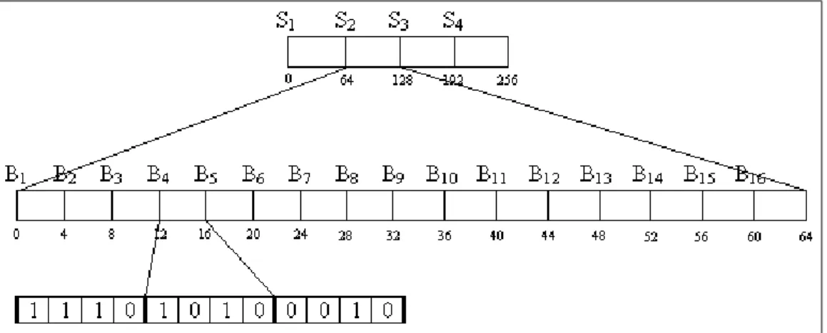
For example, for a bitmap A of size 250 number of superblocks will be 4 = ⌈log2502_n⌉. The extra 6 bits are due to the round up operation and are padded

with zeros. There will be 16 = 2_⌈logn_⌉blocks with 4 =_⌈(logn)/2_⌉bits each. To ﬁnd Rank1(A,78) compute the superblock with 86/64 = 1 remainder 14, therefore superblock S2. The block 14/4 = 3 remainder 2, therefore block

B4. Retrieving the classc= 2 the block and the index i= 5 we consult the table G2(2,5). Now Rank1(A,78) is obtained adding the rank of S2 plus the relative rank of B4 plus the rank returned by tableG2.

(27)

Figure 2.5: The four superblocks are on top, then the 16 blocks corresponding to the second superblock and at the bottom the binary representation of the third, fourth and ﬁfth blocks.

tree is a tree whose leaves represent the symbols of the alfabet. Given a position i in sequence T the algorithm will travel through the nodes until it reaches a leaf and discovers the corresponding alphabet symbol. This process will allow us to compute Rank and Select.

The root is associated to the whole sequence T= t1...tn. The left and right

child of root will each have a part of the sequence associated to a half of the alphabet. This is done by dividing the alphabet of size σ in σ/2, the left child will have a sequenceW with the symbols with value smaller or equal to

σ/2 and the right child larger thanσ/2. A position in the left child sequence is given by concatenating all ti < σ/2 in T. Notice that for every node v

(28)

Figure 2.6: For example the text "mississippi", has a alphabet bit coding showed on the left. That bit coding generates the two dimensional bit array shown on the right.

We can use the bitmap at a node and the Rank and Select operations to map to a child node. To compute the generalized Rank, resp Select we iteratively apply Rank, resp Select, travelling through the wavelet tree. To compute Rank we descend from the root to a leaf. To compute select we move upwards from a leaf to the root. To get the caracter at positioni,ti, we

travel the tree by going left or right depending on the value of the bit vector of the node. If the position i has 0 in node’s v bitmap, W, the ti is on the

left child, else it is on the right child. If the left is chosen we should update

i_←Rank0(W, i). Else if we go to the right and update i_←Rank1(W, i).

(29)

For example we show how to computeRank of caracter "p" inposition= 11 ofT. Note that the representation of "p" is "0,1,1", therefore we will compute

Rank0, Rank1 and Rank1 in succession for each node visited. The ﬁrst bit in the binary representation of "p" is 1, therefore we should go to the left child and position _← Rank0(001101100000,11) results in position = 7. The second bit for caracter "p" in the alphabet bitmap is "1", therefore we will go to the right child and update position _←Rank1(10001100,7) which computes position= 3. Finally the third bit for caracter "p" is "1", therefore we should go to the right child and position _← Rank1(011,3) results in

position= 2. The result ofRankp(mississippi$,11) is found as we reach the

leaf. There the current position= 2 indicates the rank of the symbol "p" at 11.

To compute Selectc(T, position) the algorithm will start at the leaf of c.

Since the representation of "i" is "0,0,1" we will compute Select1, Select0 and Select0 successively. We will climb the tree up to the root. At each node v it updates position_←Selectb(W, position) (b is 0 or 1 depending on

the corresponding bit in the representation of "i"). For example ﬁnding the position of the second "i" in T is Selecti(mississippi$,2). First we travel to

the leaf of symbol "i", this can be done with a direct mapping from a array of the alphabet to the leaves. Since the current node is the right child of its parent position _← Select1(11110,2). We travel to the parent and now

position = 2. The next upward climb is from a left child and therefore

position _← Select0(10001100,2) so position = 3. Reaching the root again from a left child position _← Select0(001101100000,3) computes the ﬁnal position position= 4.

(30)

2.2.3 FMIndex

The FMIndex is a full text index which occupies minute space. Since it compresses and respresents the text the FMIndex is a compressed self index. The strengh of this index relies on the combination of the Burrows Wheeler compression algorithm with the wavelet tree data structure.

The Burrows Wheeler Transform (BWT) is a reversible transformation of a text. A text T of sizenis represented in a new text with the same caracters in a diﬀerent order but normally with more sequential repetitions and therefore easier to compress. The stages of the BWT are explained in three steps.

1. A new caracter with lexicographical value smaller than any other in T is append at the end. Let it be "$".

2. Build a matrix M such that each row is cyclic shift of the string T$, then sort the rows in lexicographic order.

3. The text L is formed by the last column of M and is the result of the BWT.

The Figure 2.8 ilustrates the Burrows-Wheeler transformation of a text. The text "mississippi" becomes "mississippi$" after step 1. Using cyclic shifts the matrix on the left side of figure is generated. Sorting those rows by lexicographic order creates the matrix on the right. L is a permutation of the original text T and so are all other columns in M. Column F is a special case because it is the lexicopraphically ordered caracters of T$. The relation between matrix M and suffix arrays becomes evidente if we notice that sorting the rows of M is sorting the suffixes of T$.

(31)

Figure 2.8: To the left of the figure is the matrix with successive cyclic shifts of text "mississippi$". On the right of the figure is the matrix after lexicographical row ordering with the last and first collumns in boxes.

in L precede the caracters in F. A important function is the last to ﬁrst col-umn mapping (LF). LF describes a way to obtain the caracter position in F corresponding to a given position in L with functions C and Occ [19].

LF(i) = C(L[i]) +Occ(L[i], i)

For example the "p" in mississippi is at position 7 of L. We wish to know

LF(7) so we calculateC(”p”) = 6andOcc(”p”,7) = 2. FinallyLF(7) = 6+2

shows that the result of moving caracter "p" from L to F results in row 8. The next operation is fundamental to understand how LF mapping generates and returns the string T in reverse order. If T is the ith caracter in L then the caracter at position k₋1 is at the end of the row returned by LF(i).

T[k₋1] =L[LF(i)]

(32)

caracter in row 12 is the ﬁrst "i" in the text. Iterating over L[LF(i)] the FMIndex returns the full text from the compressed representation of L.

Based on this idea Ferragina and Manzini [4] proposed the backward search procedure. The backward search ﬁnds a patternP[1, n] within the text ﬁnd-ing caracters of the pattern from right to left. This is usefull for the FMIndex since the LF mapping returns caracters right to left. In matrix M notice that all answers to a particular pattern are lexicographically similar and are put in sequential rows. These rows are delimited by the sp and ep indexes, sp

indicates (in lexicographic order of M) the ﬁrst row with the pattern and ep

the last row.

At the start of the search sp is the position of the ﬁrst lexicographic oc-currence of the last caracter of pattern. Since ep points to the last row in the sequence it should be the row before the next lexicographical caracter. Therefore sp = C(P[m]) + 1 and ep = C(P[m] + 1). The backward search starts with the character in positioni=m. The algorithm will use a caracter in position P[i] at each step until it reaches the start of pattern and i = 1 and returns the interval [sp, ep].

The cicle that moves P[i] from i = m down to i = 1 and updates sp and

ep uses the number of occurrences in L of caracter P[i] up to position sp

or ep. The function for sp is sp = C(c) +Occ(c, sp ₋1) + 1 and for ep is ep= C(c) +Occ(ep).

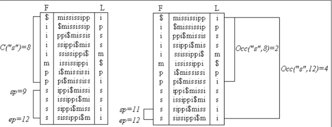
For example we will search for pattern "ss", see Figure 2.9 within "mississippi" with backward search. First c = P[m] so c = ”s”, hence sp = C(”s”) + 1

so sp = 9, ep = C(”s” + 1) so ep = 12. Now we proceed to the begining of the pattern as c = [m ₋1] so c = ”s”. We update sp and ep, sp =

C(c) + Occ(c,9 ₋ 1) + 1 so sp = 8 + 2 + 1, ep = C(c) + Occ(c,12) so

(33)

Figure 2.9: Matrix M of the Burrows Wheeler Transform with operations computed during a backward search.

The space required by FMIndex isnHk+o(nlogσ) bits, withk ≥αlogσlogn.

The time to count the number of occurrences is O(m) and time to return l

letters is O(σ(l+ log1+ǫn)), ǫ is any constant larger than 0 [19].

2.3 Static Compressed Suﬃx Trees

Three recent compressed and static suffix trees are discussed in this chapter. These are different approaches and studying them is important to under-stand why the dissertation approached this work. First we present the CST proposed by Sadakane et al [24], section 2.3.1. Section 2.3.2 presents the FCST proposed by Russo, Arlindo and Navarro [12] which is compared with the CST described in 2.3.1. The compressed suffix tree by Fischer et al [5] is presented in section 2.3.3.

2.3.1 Sadakane Compressed

(34)

O(nlogn) bits which compared n with the size of a alphabet shows a huge achievement. For example DNA has a alphabet of size 4, the size of the human genome is 700 megabytes, hence in this case logn/logσ is at least 14,5. A classical suﬃx tree for such a problem would span a impressive 40 gigabytes [10].

The problem addressed by Sadakane[24] is to remove the pointers from the representation. As for every pointer it is necessary lognbits such a result uses at least O(nlog n). To reduce space use Sadakane replaced the commonly used tree structure with a balanced parentheses representation of the tree. For a tree withnnodes the parentheses representation uses 2n+o(n) bits[18]. A suﬃx tree with text of size n has at mostn leaves, n₋1 internal nodes for a total 2n₋1 nodes. Therefore a tree can be represented in 4n+o(n) bits with the parentheses notation.

Figure 2.10: At the top of the figure is a representation of depth first ordering of the suffix tree for "mississippi". The table at the bottom represents the order of parentheses for this tree. The first row is the index of the array, the second is the node number in the suffix tree and the third is the paretheses representation.

(35)

node is visited add a left parentheses, then visit all the nodes in the sub-tree, after all sub-nodes are visited add a right parentheses[18]. The nodes in the tree are represented by a pair of parentheses. This representation can be stored by using a bit per parentheses. Therefore the parentheses tree representation is stored in a bitmap. This is a signiﬁcant improvement provided the usual navigational operations are supported.

The total space for this suﬃx tree is nHk + 6n +o(n) bits. The nHk

ac-counts for a compressed suﬃx array which is necessary to compute SLink

and read edge-labels, the remaining space is for auxiliary data structures such as the parentheses representation and a range minimum query data struc-ture. Interestingly in a note for future work Sadakane referred to the 6n

space problem in the structure. That 6n problem was addressed by Russo, Arlindo and Navarro[12].

2.3.2 FCST

The fully compressed suffix tree proposed by Russo, Arlindo and Navarro [12] uses the less space to represent a suffix tree while loosing some speed. There is an implementation by Russo that achieves optimal compressed space for the first time.

The FCST is composed of two data structures. A sampled suffix tree S and a compressed suffix array CSA. The sampled suffix tree plays the same role in the FCST as Sadakane’s parentheses tree in the CST. The reason why the sampling is used instead of storing all the nodes is that suffix trees are self-similar acording to the following lemma:

Lemma 1 SLink(LCA(v, v′_{)) =}_LCA₍_SLink₍_v₎_{, SLink}₍_v′₎₎

(36)

both nodes is reached with X.α, LCA(v, v′_{) =} _X.α_{. The SLink is applied}

to v, v′ _and _LCA₍_{v, v}′_{)and obtain resp} _{α.Y β}_, _α.Z.β _and _α_{. Notice that} LCA(α.Y β, α.Z.β) = α and therefore

SLink(LCA(v, v′_{)) =} _LCA₍_SLink₍_v₎_{, SLink}₍_v′_)).

The sampled tree explores this similarity, it is necessary that every node is, in some sense, close enough to a sampled node. This means that if the computation starts at a nodev and follow suﬃx links successively, i.e. apply

SLink on the result of SLink of v several times, in a maximum of δ steps the computation reaches a node sampled in the tree. This is an important property for a δ sampled tree. Also because the SLink of the root is a special case that has no result, the root must be sampled. The nodes picked for sampling are those that SDep(v)_≡δ/2 0 such that exists a node v and a string _|T′_{| ≥} _δ/_{2 and} _v′ ₌_LF₍_T′_{, v}_{), i.e. the remander of} _SDep₍_v_{) and} _δ/₂

is 0.

The sampled suﬃx tree allows the reduction of space usage on the total tree. A suﬃx tree with 2n nodes with a implementation based on pointers uses

O(nlogn) bits. A sampled tree requires only O(n

δ logn) bits, to use only

o(nlogδ) bits of space and in this dissertation δ=_⌈(log_σlogn) logn_⌉.

Sadakane uses a CSA [9] that requires space of 1

ǫnH0+O(nlog logσ) bits. In

the FCST the CSA is an FM-index[7]. It requires nHk+o(nlogσ) bits, with

k _≥ αlog_σlogn and constant 0 < σ < 1. Note that although Sadakane´s CSA is faster it would use more space than is desirable.

It is important to map the information from the sampled tree to the CSA and vice-versa. For this goal the operations in the sampled suﬃx tree include

LCSA(v, v′₎_{, LSA}₍_v_{) and} _{REDU CE}₍_v_{). These operations are explained}

(37)

Figure 2.11: The figure shows the suffix tree of the word mississippi. Nodes filled in gray outline are sampled due to the number of suffix links and to the string depth. The sampling chosen is 4 so nodes are sampled if SDepis multiple of 2, and if exists a suffix link chain of length multiple of two. The thick arrows between leafs are suffix links.

It is now explained how the FCST computes its basic funcion. If v and v′

are nodes and SLinkr₍_LCA₍_{v, v}′_{)) =}_ROOT_, _d₌_min₍_{δ, r}_{+ 1):}

Lemma 2

SDep(LCA(v, v′_{)) =}_max

0≤i≤d{i+SDep(LCSA((SLinki(v), SLinki(v′)))}.

The operation LCSA is supported in constant time for leaves. SDepis only applied to sample nodes so its information is stored in the sampled nodes. The other operation needed to implement the previous lemma is SLink.

(38)

wherevland vr are the left adn right extremes of the interval that represents

v [3]. This is extended to SLinki₍_v_{) =}_LCA₍_ψi₍_vl₎_{, ψ}i₍_vr_{)). Remember that}

all ψ answers are computadle in constant time. A lemma proded by Russo et al. concludes:

Lemma 3

LCA(v, v′_{) =} _LCA₍_min_{_{vl, vl}′_}_{, max}_{_{vr, vr}′_}₎

From the previous lemma, the deﬁnition of ψ and lemma 2 concludes:

SDep(LCA(v, v′_{)) =}

max0≤i≤d{i+SDep(LCSA((ψi(min{vl, vl′}), ψi(max{vr, vr′})))}

Therefore SLink is not necessary to compute LCA. Hence it is also con-cluded, using the i from lemma 2 :

Lemma 4:LCA(v, v′_{) =}_LF₍_v_[0_..i₋_1]_{, LCSA}₍_SLinki₍_v₎_{, SLink}i₍_v′₎₎

Therefore it can be solved with the same properties that solved lemma 3.

LCA(v, v′_{) =} _LF₍_v_[0_..i₋_1]_{, LCSA}₍_ψi₍_min_{_{vl, vl}′_}₎_{, ψ}i₍_min_{_{vr, vr}′_}₎₎

The operation LET T ER in FCST is solved with the following:

LET T ER(v, i) = SLinki₍_v_{)[0] =}_ψi₍_v l)[0].

Operation P arent(v) returns the smallest between LCA(vl−1, vr and

LCA(vl, vr + 1). This works because suﬃx trees are compact. Child of a

(39)

Table 2.1: The table shows time and space complexities for Sadakane static CST and Russo et al. FCST. The ﬁrst row has space use and the remaining rows are time complexities. In the left collumn are operations, the middle column has time complexities for Sadakane static CST and the right column has FCST time complexities.

Sadakane CST Russo et al. FCST Space in bits nHk+6n+o(nlogσ) nHk+o(nlogσ)

SDep log_σ(logn) logn log_σ(logn) logn

Count/Ancestor 1 1

Parent 1 log_σ(logn) logn

SLink 1 log_σ(logn) logn

SLinki _log

σ(logn) logn logσ(logn) logn

LETTER(v, i) logσ(logn) logn logσ(logn) logn

LCA 1 log_σ(logn) logn

Child log(logn) logn (log(logn))2_log

σ

TDep 1 ((log_σ(logn)) logn)2

WeinerLink 1 1

2.3.3 An(Other) entropy-bounded compressed suﬃx

tree

Fischer et al. [5] presented a compressed suffix tree with sub-logarithmic time for operations and consuming less space than Sadakane’s compressed suffix tree, detailed in section 2.3.1. They used two ideas to achieve theses results, first reducing space used for LCP information and secondly discarding the suffix tree structure using the suffix array intervals to represent tree nodes and using the LCP information to navigate the tree.

(40)

number of runs in ψ. Encoding this information with additional structures and reducing U they obtain nHk ×(2 log_H1k +

1

ǫ +O(1)) bits to store the

LCP information, whereǫ is a constant 0<ǫ<1.

They deﬁne the next smaller querie, N SV and the previous smaller querie

P SV. For a sequence,I, of integers the NSV of positionireturnsj such that

j > i, I[j]< I[i] and no position between i and j has a smaller integer in I. The PSV is identical to N SV with j < i. Remember theRM Q is two index positions (i, j) and I to return the index of the smallest integer between i

and j argmini≤k≤jI[k].

Figure 2.12: The ﬁgure shows a LCP table and the operations required to perform SLink(3,6) with RM Q and P SV, N SV.

The RM Q together withψ, N SQand P SQis enough to navigate the suﬃx tree. For an example see Figure 2.12, given a node v(vl, vr) the suﬃx link

is computation is shown. First notice that RM Q in the interval [vl, vr] will

(41)

function, available in the CSA, to vl and vr] and obtain [x, y]. Now ﬁnd k

with a LCP(k) = h-1 using RM Q in the interval [x, y], ﬁnally to ﬁnd the node’s right and left limits [v′

l, v′r] apply P SV to x and N SV to y.

They achieve a total space of nHk×(2 log_H1k +

1

ǫ +O(1)) +o(nlogσ) bits

of space while FCST uses nHk+o(nlogσ) bits. The extra factor tends to

zero if nHk is close to zero, however it is not common for the entropy to

be close to zero. This solution presents a middle point between FCST and Sadakane’s CST in both speed and space. Moreover this solution is static, i.e. it cannot be updated whenever the text changes.

2.4 Dynamic Compressed Indexes

Dynamic FCST’s use dynamic bit sequence as a auxiliary structures. One such dynamic bit sequence, proposed by Makinen and Navarro [15], is pre-sented in section 2.4.1. Section 2.4.2 presents the dynamic CST by Chan et. al [3], which is a alternative to the dynamic FCST proposed by by Russo, Arlindo and Navarro [22]. The dynamic FCST is described in section 2.4.3 which ends with the comparison of the dynamic FCST and the dynamic CST.

2.4.1 Dynamic Rank and Select

A structure is dynamic if it supports the insertion and removal of text from a collection. Makinen and Navarro obtained a dynamic FMIndex by ﬁrst presenting a dynamic structure for Rank, Select and using a wavelet tree over the BWT[15]. They show how to achieve nH0+o(n) bits of space and

O(log(n)) worst case for Rank, Select, insert and delete.

(42)

and blocks, while the superblocks are in the leaves of a tree the blocks are arranged in the superblocks.

The tree used to store the superblocks is a binary tree, a red black tree, with additional data in the nodes to compute operations such asRank andSelect

while traversing the tree. Consider a balanced binary tree on a bit vector

A = a1...an, the left most leaf contains bits a1a2...alogn, the second left leaf

alogn+1+alogn+2...a2(logn+1) through to the last leaf. Each node v contains counters p(v) andr(v) resp counting the number of positions stored and the number of bits set to "1" in the subtree v. This tree with log(n) size pointers and counters, requires O(n) bits of space[15].

The superblocks contain compacted bit-sequences but we will explain the operations as if they are not compacted. To compute Rank(A, i) we use the tree to ﬁnd the leaf with position i. We use a variable rankResult that is initially set with value 0. We travel the tree downwards to the leaves, we use the value of p(lef t(v)), if it is smaller than i we go to the left subtree of v. Otherwise we descend to the right node, in which caseiandrankResultmust be updated asi=i₋p(lef t(v)) andrankResult=rankResult+r(lef t(v)). The desired leaf is reached in O(log(n)) time and Rank(A, i) uses extra

O(log(n)) time to scan the bit sequence of the corresponding leaf. When the leaf is reached the result of scanning the bit sequence for Rank is added to

rankResult. Select(A,i) is similar but we switch the r(v) and p(v) roles.

As an example we will compute Rank1(A,10), see Figure 2.13. Since 8 =

p(lef t(root)) is smaller than 10 we descend to the right child of the root and update rankResult = r(lef t(root)) and i = 2 = 10 ₋p(lef t(root)). The left child of the current node has p = 4 which is larger than i, therefore we descent to the left child. The current node is a leaf and we scan the bitmap to ﬁnd the local rank of positioni= 2. The local rank plusrankResultgives a total rank of 4.

(43)

Figure 2.13: The ﬁgure shows a binary tree with pandr values at the nodes and bitmaps at the leaves. The path in bold is used to compute Rank of position 10.

superblock operations. To find where to insert or delete a bit we navigate the red black tree down to the leaf, like inRank, and update the bit-sequence by performing the necessary changes. The next operation is updating the p(v) and r(v) functions in the path from the leaf up to the root. Eventually insert and delete will generate overflow or underflow. If we insert a bit in a leaf the block is bitwise shifted and the bit inserted. This however will make a bit fall of the end of the block which has to be inserted on the next block. The underflow problem is similar and both overflow and underflow are discussed further on. After these split and merge operations the tree must be updated with new values for p(v) and r(v) as well as rebalancing the tree. If the bitmaps are compacted the underflow and overflow are handled differently.

(44)

logn

2 bits. The universal table Rin the superblock computes theRank values for each block, therefore Rank in the superblock is computed with the help of table R.

To compute Rank in a superblock we scan through the blocks and table R

adding eachRank until we are at the block with the query position. The bits within the block are scanned until we reach the desired position andRank is computed in O(logn) time. Select is similar to Rank because the universal table indicates the number of bits within a block. Therefore we travel the blocks to the block that contains the position querie. At that block we scan the bits and retrieve Select.

In the structure presented by Veli and Navarro the block and superblock have no wasted bits, therefore whenever a bit is inserted or deleted a overflow or underflow problem arises. Overflow propagation to the adjacent leaves may not be fixed with a constant number of block splits. We will now discuss the solution to the underflow problem.

In this structure whenever a bit is inserted a bit shift occurs. A block were a bit is inserted will have a block overflow due to the extra bit that needs to be inserted in the next block. This propagates through all the blocks in the superblock and eventually reaches the end of the superblock causing a superblock overflow. To limit the propagation of overflow we will add a partial superblock at every O(logn) superblocks. This superblock uses

(45)

until we reach it. If there is no partial superblock we propagate through

O(logn) superblocks and create a partial superblock at this location. In both situations we have to travel O(logn) superblocks and guarantee that every superblocks is at leastO(logn) distant from other superblocks. However the partial superblocks may overflow, in which case they are no longer partial. We create a new partial superblock after it and the partial superblock that overflows becomes a normal superblock. When a partial superblock overflows it will in some cases have a partial block at its end. They solve this by simply moving this block to the new partial superblock end. Other overflow blocks will fill the rest of the partial superblock.

Another operation is the removal of one bit that causes underflow. We ensure that the superblocks are always full. If some underflow happens in the end of the superblock, we use the next superblock and move some blocks back. This propagation is similar to overflow propagation. If we reach a partial superblock the problem is solved and propagation stops. If the search for a partial superblock exceeds 2O(logn) steps we allow the underflow in the

O(logn) superblock and it becomes a new partial superblock. If a partial superblock becomes empty it is removed from the tree.

Insertion and deletion of bits will require the update of p(v) and r(v) values from the leaf up to the root. However the propagation problem aﬀects only

O(logn) superblocks. When we ﬁnd the leaf that we wish to create or delete, the red-black tree uses constant time to rebalance, this will addO(logn) time per insertion or deletion. When propagating the coloring of the red-black tree and updating the p(v) and r(v) values the O(logn) blocks are contiguous, therefore the number of ancestors does not exceed O(logn) +O(logn) =

O(logn). The overall work needed for this maintenance is O(logn).

Veli and Navarro achieve a structure that manages a dynamic bit sequence in

(46)

2.4.2 Dynamic compressed suﬃx trees

Chan et al. proposed, in 2004, a dynamic compressed suﬃx tree that uses

O(nlogσ) bits of space[3]. They use a mixed version of a CSA plus a FMIn-dex to speed up their updates, at the time CSA and the FMInFMIn-dex were used to provide complementary operations. However new versions of the FMIndex can also compute the ψ function hence replacing the CSA[3]. The structures used are named COUNT, MARK and PSI respectively related to the LF, the SA and the ψ functions. The MARK structure computes SA[i], to do this it stores some values from the SA array and determines the other values with the COUNT structure[3]. The COUNT and PSI structures are sup-ported by an FMIndex that supports insertions and deletions of texts T′ _in O(_|T′_|_log_n_).

Recall that Occ(c, i) returns the number of occurrences of symbol "c" up to position i of the BWT. For example, a bitmap of size n for character "c" with each occurrence in the text is computable, notice that Rank1(i) over this bitmap will return Count(c, i). These bitmaps can be stored in the structures presented in the previous section. To compute MARK they use two RedBlacks that store values explicitly. Adding all the red blacks the total space is O(nlogσ) bits. The insertion and deletion of a character from the text uses O(log n) time while ﬁnding a pattern of size m uses

O(mlog n+occlog2n).

This approach is one of the few dynamic compressed suﬃx trees available and therefore is a tool to judge our own dynamic CST performance. Chan et al.[3] CST usesO(nlogσ), however the dynamic FCST usesnHk+o(nlogσ),

(47)

Dynamic Parentheses Representation

Chan et al.[3] proposed a CST in 2007, in this dissertation there is interest in the approach to the LCA problem. They proposed a way to store the topology of a suffix tree inO(n) bits of space. The parentheses representation of the tree topology creates a bitmap of 2n bits that is processed to find matching and enclosing parentheses. This is done with two structures that complement each other and answer LCA queries. The two structures are dynamic, the first supports delete and insert in O(_{log log}logn_n) time, the second supports these operations in O(logn).

The ﬁrst structure computes matching parentheses. It is a B-tree with the parentheses bitmap divided in blocks of size from _{log log}log2n_n to 2_{log log}log2n_n. The bitmap is distributed on the leaves of the tree, i.e. and concatenating the leaves in order returns the original parentheses bitmap.

The second structure determines the LCA, witch is the same as double en-closing parentheses, it is a red black tree with the parentheses bitmap di-vided in blocks of size from logn to 2 logn. The bitmap is distributed over the leaves of the tree. Concatenating the leaves in order returns the original parentheses bitmap and ﬁnd the nearest enclosing parentheses using auxiliary structures in the nodes of the red black.

Matching Parentheses

The matching parentheses of a position i in the parentheses representation is found consulting position i + 1 and if necessary computing the nearest enclosing parentheses.

(48)

Figure 2.14: The figure represents the computation of the matching parenthe-ses for index position 15 and position 18 over the parentheparenthe-ses representation of the suffix tree for "mississippi". The first row is the index position of the bitmap. The second row is the depth first numbering of the nodes and the third is the parentheses represented by the bitmap. The fourth and fifth rows are the steps used to compute the matching open parentheses and the sixth and seventh rows are the computation of the matching closing parentheses.

search incrementing the index position to ﬁnd the corresponding enclosing parentheses. For each index position visited add 1 to a counter if it is a opened parentheses and subtract 1 if it is a closed parentheses. In this example in Figure 2.14 travel from index 19 to index 31, until our counter reaches -1. Therefore the matching parentheses of 18 is 31.

The index position 15 corresponds to a closed parentheses, therefore search backwards for the corresponding enclosing open parentheses. For each index position visited add 1 to the counter if it is a closed parentheses and subtract 1 otherwise. In this example in Figure 2.14 travel from index 14 to index 4 until the counter reaches -1, therefore the matching parentheses of 15 is 4.

The structure presented by Chan et al. [3] proposes that for each node

v of the B-tree, information is stored for the computation of size, closed,

opened, nearOpen, f arOpen, nearCloseandf arClose. size stores the num-ber of parentheses in the sub-tree of v, closed and opened store the total of closed and opened parentheses in the sub-tree. The structures nearOpen

Universidade Nova de Lisboa Faculdade de Ciências e Tecnologia Departamento de Informática An Implementation of Dynamic Fully Compressed Suffix Trees