Landing on the right job : a machine learning approach to match candidates with jobs applying semantic embeddings

Landing on the right job: a Machine Learning

approach to match candidates with jobs

applying semantic embeddings

2

Luís Matos Pombo

Work project presented as partial requirement for obtaining

the Master’s degree in Advanced Analytics

Landing on the right job: a Machine Learning

approach to match candidates with jobs applying

semantic embeddings

3

Title:Landing on the right job

Title:Landing on the right job

Luís Matos Pombo

Luís Matos Pombo

MAA

5

NOVA Information Management School

Instituto Superior de Estatística e Gestão de Informação

TITLE: LANDING ON THE RIGHT JOB: A MACHINE LEARNING APPROACH

TO MATCH CANDIDATES WITH JOBS APPLYING SEMANTIC EMBEDDINGS

by

Luís Matos Pombo

Work project presented as partial requirement for obtaining the Master’s degree in Information Management, with a specialization in Advanced Analytics

6

ABSTRACT

Job application’ screening is a challenging and time-consuming task to execute manually. For recruiting companies such as Landing.Jobs it poses constraints on the ability to scale the business. Some systems have been built for assisting recruiters screening applications but they tend to overlook the challenges related with natural language. On the other side, most people nowadays specially in the IT-sector use the Internet to look for jobs, however, given the huge amount of job postings online, it can be complicated for a candidate to short-list the right ones for applying to. In this work we test a collection of Machine Learning algorithms and through the usage of cross-validation we calibrate the most important hyper-parameters of each algorithm. The learning algorithms attempt to learn what makes a successful match between candidate profile and job requirements using for training historical data of selected/reject applications in the screening phase. The features we use for building our models include the similarities between the job requirements and the candidate profile in dimensions such as skills, profession, location and a set of job features which intend to capture the experience level, salary expectations, among others. In a first set of experiments, our best results emerge from the application of the Multilayer Perceptron algorithm (also known as Feed-Forward Neural Networks). After this, we improve the skills-matching feature by applying techniques for semantically embedding required/offered skills in order to tackle problems such as synonyms and typos which artificially degrade the similarity between job profile and candidate profile and degrade the overall quality of the results. Through the usage of word2vec algorithm for embedding skills and Multilayer Perceptron to learn the overall matching we obtain our best results. We believe our results could be even further improved by extending the idea of semantic embedding to other features and by finding candidates with similar job preferences with the target candidate and building upon that a richer presentation of the candidate profile. We consider that the final model we present in this work can be deployed in production as a first-level tool for doing the heavy-lifting of screening all applications, then passing the top N matches for manual inspection. Also, the results of our model can be used to complement any recommendation system in place by simply running the model encoding the profile of all candidates in the database upon any new job opening and recommend the jobs to the candidates which yield higher matching probability.

7

ACKNOWLEDGEMENTS

To my parents and brother, for their unconditional love.

A special thank you to Kira for her invaluable support, in so many ways. To my dog Pierre, for being my company in the lonely days.

To Prof. Vanneschi for his inspirational classes.

To Kristen and Asimina, for their friendship and companionship through this master program and beyond.

To Illya for his Computation I classes, a huge asset which has opened my opportunities.

To my fellow colleagues Ariana, Esdras, Bernardo, Maria and Nicolas for the great experience of working with such smart and kind people.

8

Index

1.1. Latent Semantic Analysis (LSA)... 16

1.2 Variance Inflation Factor (VIF) ... 17

2. Machine Learning ... 18

2.1 Supervised Learning ... 18

2.1.1 Logistic Regression(LR) / Single Layer Perceptron (SLP) ... 18

2.1.2 Multilayer perceptron (MLP) / Artificial Neural Networks (NN) ... 19

2.1.3 Decision trees ... 20

2.1.4 Random Forests (RF) ... 21

3 Variable Selection ... 21

3.1 Recursive Feature Elimination (RFE) ... 21

4. Filtering ... 21

5. Cross-validation (CV) ... 22

6 Natural Language Processing (NLP) ... 22

6.1 Word embeddings - Word2vec ... 22

D. Data ... 23

E. Methodology ... 24

No Free Lunch Theorem ... 24

Data modelling in practice ... 24

Software ... 25

F. Data transformation ... 25

1. Building the target variable ... 25

2.People features - create people dataset ... 26

2.1. Extracting people skills and tags ... 27

3. Job ad features – create job ads dataset ... 29

3.1. Extracting required skills and nice-to-have skills ... 30

G. Experiments ... 30

Experiment-set A ... 31

9

1. Skills-matching ... 31

2. Profession-matching... 32

The final match value is computed by dividing the distance 𝑆𝑛 by the length of the longest of the two strings. ... 32

3. Location-matching ... 32

4. Additional features ... 34

Data preprocessing and feature selection ... 35

Feature selection ... 37 Modelling ... 38 Logistic Regression ... 38 Multilayer Perceptron ... 39 Random Forests... 39 Results: experiment-set A ... 40 Experiment-set B ... 41

Feature engineering – semantic embedding ... 41

Latent Semantic Analysis (LSA) ... 41

Word2vec ... 42 Results – Experiment-set B... 42 Discussion of results ... 43 H - Future work ... 44 I – Conclusion ... 46 J - Bibliography ... 48 Appendix ... 52

Table of figures

TABLE 2 - CANONICALIZED TAGS IDS TRANSFORMED... 27

TABLE 3 - SKILLS TABLE AFTER TRANSFORMATION ON TAG IDS FIELD ... 28

TABLE 4 - TAGS TABLE ... 28

TABLE 5 - SKILL TAGS PER PERSON ... 29

TABLE 6 - JOB AD SKILLS ... 30

TABLE 7 - TRANSFORMED JOB AD SKILLS ... 30

TABLE 8 - VIF SCORES PER FEATURE BEFORE REMOVING BASELINE CLASSES IN CATEGORICAL VARIABLES ... 36

TABLE 9 - VIF SCORES PER FEATURE AFTER REMOVING BASELINE CLASSES IN CATEGORICAL VARIABLES ... 36

10

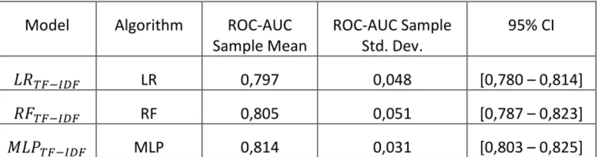
TABLE 11 - BEST RESULTS PER MACHINE LEARNING ALGORITHM USING THE TF-IDF ENCODING OF SKILLS ... 41

TABLE 12 - RESULTS IN TERMS OF ROC-AUC AFTER APPLYING THE MLP FINE-TUNED WHERE SKILLS ARE REPRESENTED AS SEMANTIC VECTORS ... 43

TABLE 13 - DATA SUMMARIZATION - PART I ... 52

TABLE 14 - DATA SUMMARIZATION - PART II ... 52

TABLE 15 - APPLICATION STATES ... 53

TABLE 16 - FIELDS OF TABLE PEOPLE ... 54

TABLE 17-FIELDS OF TABLE APPLICATIONS ... 55

TABLE 18 - FIELDS OF TABLE APPLICATION AUDIT ... 55

TABLE 19 - FIELDS OF TABLE JOB ADS ... 57

TABLE 20 - FIELDS OF TABLE COMPANIES ... 59

TABLE 21 - FIELDS OF TABLE TAGS ... 59

TABLE 22 - FIELDS OF TABLE SKILLS ... 59

FIGURE 1: RECRUITMENT PROCESS ADAPTED FROM PROSPECT AND JRS SURVEY ... 15

FIGURE 2 - CURATOR-DEFINED TARGET. ON AXIS 0 WE HAVE THE CLASS AND ON AXIS 1 WE HAVE THE NUMBER OF OBSERVATIONS ... 26

FIGURE 3- GROUPING JOB ADS FIELDS ... 29

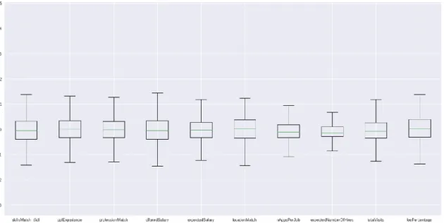
FIGURE 4- BOXPLOT CHART REPRESENTING VARIABLES PRIOR APPLYING SAVITZKY–GOLAY FILTER ... 37

11

A. Introduction

In the field of job recruitment, Internet has become a major channel for recruiters to publish job postings and attract candidates, whereas looking and applying for jobs have become mostly tasks that candidates perform online(Malinowski, Keim, Wendt, & Weitzel, 2006). While Internet certainly allows reaching a wider audience on the recruiters’ standpoint and makes job applications more convenient on the candidates’ standpoint, two problems arise: on one side, there is a tremendous amount of job postings online in different job portals and company’s career sections. This situation makes the candidate’s task of short-listing jobs a tedious and time-consuming one, often deriving in sub-optimal short-listing. On the other side, certain job postings can attract hundreds or thousands of applications, making the recruiter’s task of screening all applications very challenging under businesses deadlines. To tackle the problem of job of application screening, numerous systems have been built which relied on Boolean search to filter out applications based on the inexistence of certain keywords. This technique presents several shortcomings such as ignoring the problems related with natural language including semantics and synonyms (Singh , Rose, Visweswariah , Vijil , & Kambhatla , 2010). Some more recent approaches to the problem relied on finding similarities between the applicant profile and the job profile across a multitude of dimensions such as skills, education or experience and ranking applications according to the overall similarity degree (Fazel-Zarandi & Fox, 2009), (Singh , Rose, Visweswariah , Vijil , & Kambhatla , 2010). Another approach, which uses Machine Learning was presented in (Faliagka, Ramantas, Tsakalidis, & Tzimas , 2012). However, we consider that considerable improvements to the proposed models could be reached by using start-of-the-art techniques to obtain a better representation of the jobs and the candidates’ profiles.

With regard to candidate attraction, different job recommendation systems were developed. For instance, (Paparrizos, Cambazoglu, & Gionis, 2011) built a Content-Based Recommendation System to predict the next job for a candidate. In (Yuan, et al., 2016) the authors use a Collaborative Filtering approach while performing a semantic embedding of job profiles. Yet another example which uses a Hybrid Recommendation approach can be found in (Hong, Zheng, & Wang, 2013) where the authors utilize clustering technique for clustering users and build specific recommendation systems for each cluster of users.

In this work we present a Machine Learning approach for building a model to automatically screen job application but that can also be used to complement job recommendation system. Our approach can be regarded as a hybrid one. On one side, it incorporates aspects of content-based systems because we use attributes of jobs positions and candidates for building features. On the other side, it could also be seen as an Ontology-based system as we define a set of matchings between jobs and candidates’ profiles based on the relationship that we manually draw between the attributes of these entities.

Our Machine Learning model learns what makes a successful application to a job. We achieve that by setting the target of our model as Boolean value encoding whether a certain application was pre-selected in the screening phase or not.

12 One of the major challenges is the proper encoding of jobs’ and candidates’ profiles given that many attributes are presented in natural language. To tackle this challenge, we apply tentatively a different set of strategies: TF-IDF, Latent Semantic Analysis and the start-of-the-art Word2Vec algorithm. The usage of Latent Semantic Analysis and Word2Vec has improved the overall results of our model because contrary to lexical features as in TF-IDF, these techniques explore the context of word, therefore being more resilient to problem such as synonyms which artificially degrade the similarity between the required profile for the job and the profile of the applicant.

Our model could also be deployed for purposes of job recommendation as well. In practice the difference between using the model for screening or for job recommendation is that in the former case there is an actual job application while in the latter case there is not an actual application but the potential candidate is already sitting in the database. Thus, one could ask the following question: what is the probability of person A to be a good match for job X, were person A willing to apply to it? By generalizing this question to every potential candidate in the database and every new job position, we end up with a list of top matches for each job position, therefore recommending the jobs of highest matching probability to the corresponding people. Finally, we would like to mention that this work was based on the anonymous data provided by Landing.Jobs, an IT-specialized job portal. By using the model that we have developed, the company turn application screening both cheaper and more scalable while being able to integrate their current recommendation system with our model’s output to further refine recommendations.

B. Literature review

The evolution of technology has changed that way people find and apply for jobs and the way organizations attract and receive applications. The recruitment process nowadays relies heavily on the internet as a means of communication to publish job openings, to attract applicants and to receive applications, be it through job portals or organizations’ own websites career section (Malinowski , Wendt , Keim , & Weitzel, 2006), (Desai, Bahl, Vibhandik, & Fatma, 2017). At the same time, looking for jobs online became a natural approach for most people. In job portals such as LinkedIn or Landing.jobs people create their profiles and apply for jobs using their standard profile, sometimes adding motivation letter or their custom résumé/ CV (curriculum vitae). Often, organizations’ own websites career section also allows people to create their profile to apply for multiple jobs within the organization using it. In both job portal or organizations’ own websites career section it is common to be able to activate and receive alerts of jobs matching people’s preferences and profile.

While the internet has made the application for jobs more convenient and candidates often regard the greater number of applications for jobs they make, the greater the chance of being selected for any, it sometimes leads to a huge amount of applications per job that the recruiter will have to shortlist from (Singh , Rose, Visweswariah , Vijil , & Kambhatla , 2010).

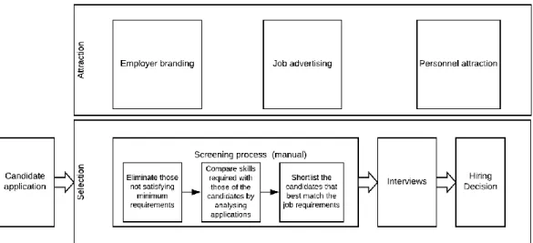
13 From another perspective, as the Internet has become a great channel for reaching and attracting a large audience, most jobs are nowadays published online, which leads to an amalgam of job postings through which the applicant has to browse through until he/she finds the ones that match his/her preferences and he/she sees has potential for success. This scenario often leads to applications for jobs that do not match so well applicant’s profile (Alotaibi, 2012). In the recruitment process context, some authors (Färber, Weitzel, & Keim, 2003) divide the recruitment process in two main phases: attraction and selection. Attraction is concerned with what happens before an application, including employer branding, job publishing and approaching potential candidates. Selection, on the other side, concern the steps after a candidate has applied. Upon the receival of applications what follows typically is a screening process intended to shortlist applications to pass to later stages where usually one or multiple rounds of interviews are conducted, tests are sometimes required and hiring decisions are made (Alotaibi, 2012). Figure X provides a generic example of a recruitment process.

In regard to the illustrated scenario, two problems arise: 1) how to efficiently screen a massive amount of applications and 2) how organizations can automatically recommend the right jobs openings to the right people. We call the former the screening problem and the later the recommendation problem.

The screening problem

To address the screening problem, organizations apply different strategies. Some opt for a purely manual approach where each application is reviewed by a human, sometimes outsourcing hiring firms to screen and shortlist candidates. To illustrate the challenge of screening applications, take the following example. Say candidate A possesses most skills required for a job but misses some critical ones, while candidate β has poorer skill set but is highly expert in some of the critical ones and yet candidate C is highly versatile, including critical skills but has only few years of experience in each. The decision to shortlist any of these candidates is not obvious and ideally should be only taken after reviewing all applications or otherwise the best application might not be found at all in the pile of all applications (Singh , Rose, Visweswariah , Vijil , & Kambhatla , 2010). Moreover, these decisions are taken under the pressure of business deadlines. This illustration presents three candidates but in practice it is hundreds or thousands of applications to be dealt by a human. That is why some organization introduce some form of Information Systems (IS) to assist on the task of screening applications. Numerous implementations relied on Boolean search, using keywords to search and filter out applications in the database which did not match those keywords (Alotaibi, 2012). However, this technique falls short on the task because it lacks the capabilities to deal with problems related with natural language such as synonyms or to capture underlying attributes such as personality trait, which according to (Singh , Rose, Visweswariah , Vijil , & Kambhatla , 2010) is the hidden reason why a large number of applications present such low compatibility with job search. More recently, new systems have been developed. For instance, in (Singh , Rose, Visweswariah , Vijil , & Kambhatla , 2010) the authors present a system which uses Information Extraction techniques to automatically mine résumés and job profiles to later rank candidates. The ranking of candidates is based on the similarity between the job requirements and the applicant profile

14 on different dimensions such as skills, education and experience. The recruiter can further refine the ranking by filtering per level of education or skills. While this system performs quite favorably in terms of feature extraction, it does not solve the problem of natural language. Another example of a screening system is the one introduced in (Faliagka, Ramantas, Tsakalidis, & Tzimas , 2012). The proposed model is built by means of Machine Learning, applying Support Vector Regression (SVR) algorithm to learn to rank candidates. For training the model, the authors used a set of features extracted from the candidate’s LinkedIn profile, such as years of education, work experience, average number of years per job as well as extraversion which is a derived feature from mining applicant’s blog posts. The model as a whole learns how to rank candidates using previous screening decisions, however given recent developments in the field of Natural Language Processing we consider that the usage of advanced techniques such as word2vec could improve results by dealing with problems such as synonyms and polysemy which are latent problems when it comes to use natural language in Machine Learning contexts.

The job recommendation problem

When a potential candidate is looking for a job, searching online has become for most people a natural way. However, searching through hundreds or thousands of jobs’ postings, a situation designated as information overload, can be overwhelming. The potential candidate finds a huge collection of jobs in different career portals and recruiter’s websites which makes the selections of positions to apply to a complex and time-consuming task. Job recommendation systems are meant to tackle that problem by providing a list of job positions to a candidate which best reflects his/her preferences and profile. Recommendation systems are widely employed for many applications, such as recommending books or movies –generally called ‘items’ – and they have been applied in the job market for more than a decade (Bobadilla, Ortega, Hernando, & Gutiérrez, 2013). Technically, recommendation systems have been split in many categories but the following three categories have been the most common:

a) Content-based Recommendation (CBR) – the idea of CBR is to suggest items to users based on similarity between the user profile and the item information. (Paparrizos, Cambazoglu, & Gionis, 2011) used this approach to build a Machine Learning model to predict the next job of a candidate using both the candidate’s profile information as well the information of the companies where the candidate had work previously. One of the challenges of CBR is the so-called overspecialization, the phenomenon in which candidatesl receive recommendations of jobs whose profiles contain multiple attributes similar to the candidates own profiles. profile while not receiving recommendation of other type of jobs which they may like more (Bobadilla, Ortega, Hernando, & Gutiérrez, 2013).

b) Collaborative Filtering Recommendation (CFR) – this technique relies on finding people similar to the target person and recommending items which similar people have liked. The similarities in Collaborative Filtering technique are concerned with people’s tastes, preferences and activities, contrary to CBR where similarity is built on top of the content of the person and the job profile. In the context of job recommendations, CFR usually relies on data about the person’s activities such as job applications, job posting clicks

15 and ratings. It is rare to find a recommendation system which relies solely on Collaborative Filtering. Among its challenges are the cold-start problems for new users and items. When a new person registers in a job portal she has never applied for a job there, therefore it is not possible to recommend her a job that someone as with the same preferences has applied to before. At the same time, when there is a new job opening, by definition no one has applied yet, so it is not possible to recommend that job to person A because no other person applied to it yet. A body of literature has attempted to solve the problem in different ways, one of which through deep learning as proposed in (Yuan, et al., 2016), where the authors build a model which learns the similarity between a new job profile and an existing one with prior applications utilizing doc2vec which is considered the current state-of-the-art deep learning algorithm for document embedding and matching. Therefore, the system can recommend the new job based on prior applications to similar jobs content-wise.

c) Hybrid Recommendation (HyR) – as seen already, all recommendation techniques have some shortcomings, therefore it is rare to find a recommendation system that uses only one technique. The hybrid approach combines different techniques to overcome the specific problems of each. In the work of (Hong, Zheng, & Wang, 2013), the authors propose clustering users into three groups based on their activity (pro-actives, passives and in-between) and apply a different recommendation technique on each group. In another work (Shalaby, et al., 2018), the authors attempt to address the challenge of cold-start in Collaborative Filtering and the rigidity of Content-based techniques. To achieve this, on one side, content-similarity between jobs is learnt by means of Machine Learning. On the other side, the authors use a statistical approach to estimate the likelihood of candidate applying for a job given their prior interactions. These intermediary results are then combined and correlated with the candidate profile and activity to provide the specific recommendations.

16 Regardless of the conceptual division between screening and recommendation, in a broader picture, the recruitment goal is to bring valuable people for the organization to fulfill its needs. Clearly a good match between people and jobs needs to consider both the preferences of the recruiter and the preferences of the candidate. It is the perspective of this work that the screening problem and the recommendation problem should be tackled as a whole. In the work of (Malinowski , Wendt , Keim , & Weitzel, 2006) the authors followed a similar idea by developing two complementary models. The first one aims to recommend people profiles (CV-recommender) that are similar to other people’s profiles previously selected by the recruiter and the second one (Job-recommender) aims to recommend jobs to people who have expressed their preference for similar jobs in the past. In the end, the authors acknowledge the need to aggregate the recommendations generated independently and propose an approach where one the first step the top candidates in terms of bilateral matching are chosen and on the second step these candidates are ranked based on their job preferences. Another work which relates to our approach is the one in (Fazel-Zarandi & Fox, 2009) who identified a set of features such as must-have skills, secondary skills, education and job experience and found the similarity degree between the job profile and applicant profile on each of these features. The work concludes by ranking the candidates based on an aggregation of the similarities through the different dimensions, whereas in our work we use machine learning to learn the parameters of a function to match the job profile and the candidate profile with a multi-dimensional input.

Lastly, in the work of (Yuan, et al., 2016), the authors find the similarities between job profiles based on the semantic representation of job profiles through means of the novel application of the doc2vec algorithm. This relates to our work in the sense that we also apply a variant of doc2vec, the word2vec algorithm to learn the semantic representation of skills and we use that representation to find the degree of similarity between applicant profile and job profile in terms of required/offered skills. Moreover, the similarity extracted from skills embedding among with a collection of other features are treated as input data for our Machine Learning application which learns what is a successful application from historical job applications.

C. Technical background

In this section we provide the technical background required in the context of this project. We describe in a high-level the variety of methods explored, the respective science fields and how these methods relate to each other. The topic-subtopic scheme that we lay here is one of many others schemes that could be drawn, as the respective science fields overlap in many domains. The details and the proper tuning of the hyper-parameter of each method in the context of our problem and data, are further explored in the experimental section.

1. Statistics

1.1. Latent Semantic Analysis (LSA)

LSA is a procedure which belongs to the Statistical subfield of Distributional Semantics. The goal of LSA is to extract the underlying concepts in a collection of documents and its respective

17

words. LSA assumes that words that are close in meaning will occur in similar pieces of text. The word frequency (sometimes multiplied by the inverse of the number of documents where the words appear) is drawn from each document and built into a matrix A. This matrix is then decomposed through Single Vector Decomposition (SVD). The resulting matrix M is a new representation of the word/document matrix. Formally:

𝑀 = 𝑈𝛴𝑉𝑇_,

where U is the unitary matrix of A (eigenvectors), 𝑉𝑇 is the conjugate transpose of the unitary

matrix of A and Σ is the diagonal matrix composed with the eigenvalues of the unitary matrix of A.

To complete the LSA procedure, one applies a low-rank approximation of M. This is done by selecting the k highest eigenvalues in matrix Σ, and subject to a minimization procedure to recreate M with a k rank.

𝑚𝑖𝑛𝑖𝑚𝑖𝑧𝑒 𝑜𝑣𝑒𝑟 𝑀̂ _{⃦ M − 𝑀̂ |⃦⃦ 𝑠𝑢𝑏𝑗𝑒𝑐𝑡 𝑡𝑜 𝑟𝑎𝑛𝑘(𝑀̂) ≤ 𝑘}

The process of low-rank approximation of M (LSA) mitigates the problem of identifying synonymy, as the rank lowering is expected to merge the dimensions associated with terms that have similar meanings, and with limited results, to mitigate polysemy problems (Pottengerb & Kontostathis, 2006).

In this project we use LSA to tackle the problem of synonymies when matching the required skills by the job offer with the offered skills of the applicant.

1.2 Variance Inflation Factor (VIF)

VIF is used as a measure the severity of multicollinearity among variables. Multicollinearity causes biased estimation, coefficient estimation instability and is a considerable obstacle to most machine-learning techniques (Dumancas & Ghalib, 2015). Collinearity is most commonly intrinsic, meaning that collinear variables are different manifestations of the same underlying construct or latent variable (Dormann, 2013).

Formally,

𝑉𝐼𝐹𝑚 = 1 1 − 𝑅2,

where 𝑉𝐼𝐹𝑚 is the VIF of the 𝑚𝑡ℎ variable, and 𝑅2 is the coefficient of determination computed from regressing variable m against the remaining ones.

The square root of VIF indicates how much larger the standard error of the variable coefficient estimation is in comparison to what it would be, were the variable uncorrelated with the other explanatory variables (Allison, 1999).

In this project, we use Variance Inflation Factor to assess the multicollinearity of our variables for the purpose of model stability.

18

2. Machine Learning

Machine learning is a field of statistics and computer science that gives computer systems the ability to progressively improve performance on a specific task with data, without being explicitly programmed. It explores the study and construction of algorithms that can learn from and make predictions on data. Such algorithms overcome following strictly static program instructions by making data-driven predictions or decisions through building a model from sample inputs (Samuel, 1959).

2.1 Supervised Learning

Supervised learning is a subfield of Machine Learning which focus on the search of algorithms that learn from labeled data to produce general hypotheses, which then make predictions about future instances. Specifically, the goal of supervised learning is to model the distribution of the class labels given the input features. The resulting model is used to predict the class label (labels in multilabel classification) of unseen instances made of the same features (Kotsiantis, 2007).

2.1.1 Logistic Regression(LR) / Single Layer Perceptron (SLP)

Logistic Regression derive both from the field of Statistics and Machine Learning. In this work, we use LR and SLP terms interchangeably. Under the Machine Learning perspective, a Logistic Regression is a special case of the Perceptron where in Statistics it is considered a special case of the Generalized Linear Regression.

Logistic regression model computes the class membership probability for one of the two categories in input vector. In matrix notation:

𝑝(𝑌 = 1|𝑋) = 1

1 + 𝑒−𝜃𝑋,

where p(𝑌 = 1|𝑋) represents the probability 1 given the input matrix 𝑋 and θ is the matrix of estimation coefficients.

The problem can be represented as a minimization problem of distance/error between the logit and the true label. A common error function (also called cost function or fitness function) is the Cross-Entropy. Formally:

𝐸 = 𝑌 log(𝑌̂) + (1 − 𝑌) log(1 − 𝑌̂),

where E is the entropy, 𝑌 is the true label and 𝑌̂ is the class estimation. The function can be minimized by multiple mean, a common one being the gradient descent (Dreiseitl & Ohno-Machado, 2002).

The advantages of LR include its weighs interpretations and model readability. They can be considered a decent first-try when we don’t know whether the classes are linearly separable or not in terms of the explanatory variables. However, for the cases where it is not possible to come

19 up with a straight line or plane to separate the classes, the Perceptron falls short, as the model will never be able to classify all instances properly (Kotsiantis, 2007).

In this project we use LR as our first approach to create a job matching model.

2.1.2 Multilayer perceptron (MLP) / Artificial Neural Networks (NN)

Multilayered Perceptron have been created to try to solve the problem of non-linearity of class separation. (Rumelhart, Hinton, & Williams, 1986). MLP can be considered a generic case of LR where between the input data and the logistic function we have intermediary/nested functions. In other words, a MLP consists of a set of functions joined together in a pattern of connections. To each function under the MLP context, the term neuron is frequently employed as the visual representation and inspiration is loosely associated with the brain. Input data is commonly called input layer, the model prediction called output layer and the intermediary layers called hidden layers. The term MLP derived afterwards in (Artificial) Neural Networks. There is a plentitude of Neural Networks topologies, but in the specific case of Feed Forward Neural Networks, where the output of each neuron travels only forward.

Learning with MLP was made possible, because of the Backpropagation algorithm (Rumelhart, Hinton, & Williams, 1986). It works by retro-propagating the error 𝐸 between the model estimation 𝑦̂ and the true value 𝑦, through the whole network.

In the output layer we differentiate the error function in order of 𝑥𝑗 to obtain the gradient to update the respective parameter:

𝑑𝐸 𝑑𝑥𝑗 = 𝑑𝐸 𝑑𝑦𝑗 𝑑𝑦𝑗 𝑑𝑥𝑗

For the hidden units, we don’t know the value of 𝑥 but we know the outputs of the previous layer neurons so we can compute how 𝐸 is affected by the output of the previous layer and their parameters. Generically:

∆𝑤 = 𝛼 𝑑𝐸

𝑑𝑤,

where ∆𝑤 is the change in the model parameters, _𝑑𝑤𝑑𝐸 is the derivative of the error in order of 𝑤 and 𝛼 is a parameter controlling the update speed, so-called, learning-rate.

One way to see backpropagation is as a generalization of the delta rule, by means of the chain rule to iteratively compute gradients for each layer so as to adjust the model parameters. MLP are a universal approximator. This means that they are capable of approximating virtually any function, with just a single hidden layer, provided that the function has a limited number of discontinuities and the number of neurons employed large enough, but not infinite (Hornik, 1989).

20 There is a plentitude of Neural Networks topologies. In this project we focus on the Feed Forward Neural Networks with a single hidden layer.

2.1.3 Decision trees

Decision trees is a learning algorithm which represents the mapping between inputs and outputs in a tree-like structure. This algorithm repeatedly splits the inputs using the feature that maximizes the separation of the data. Each node in a decision tree represents a feature and each branch represents a value that the node can assume. The feature that best divides the training data is the root node of the tree (Kotsiantis, 2007).

There are several methods to find the features that best splits the training data, such as Information Gain (Hunt, Martin, & Stone, 1966) and Gini Index (Breiman, Friedman, Stone, & Olshen, 1984).

𝐼𝑛𝑓𝑜𝑟𝑚𝑎𝑡𝑖𝑜𝑛 𝐺𝑎𝑖𝑛: 𝐺(𝑇 | 𝑎) = 𝐻(𝑇) − 𝐻(𝑇|𝑎),

where 𝐻(𝑇) is the model entropy and 𝐻(𝑇|𝑎) is the model entropy when further splitting based on the weighted entropy of the values of feature 𝑎.

𝐺𝑖𝑛𝑖 𝐼𝑛𝑑𝑒𝑥: 𝐼𝐺(𝑝) = 1 − ∑ 𝑝𝑖2 𝐽

𝑖=1 ,

where 𝑝 is the fraction of items labeled with class {\displaystyle i}𝑖𝑖 in the set and 𝐽 is the number of classes.

ReliefF algorithm is a splitting method which works a little different than the former two. ReliefF selects a feature not on the feature alone but in the context of other features. However, a majority of studies have concluded that there is no single best method (Murthy, 1998).

Decision Trees can be used both for classification and regression problems. Also, features can be either categorical or continuous. If a feature is continuous, it is implicitly discretized in the splitting process (Dreiseitl & Ohno-Machado, 2002).

By the nature of the algorithm, Decision Trees will keep on splitting the training data until all instances are correctly predicted which can create a very big model, with plenty of nodes and each node gradually with less and less instances. Such behavior can lead to overfitting so it is important to establish an adequate stop criterion. Common criteria include stopping when each child would contain less than five data points, or when splitting increases the information by less than some threshold (Shalizi, 2009).

On the other size, Decision Trees are robust to outliers, to monotonic transformations of input features, can deal with missing values an interpretable model, which is a considerable advantage in many domains.

There are multiples algorithms implementing decision trees, such as ID3, C4.5, C5.0 which use Information Gain as splitting criterion and CART which uses Gini Index.

21 In this project we use Decision Trees as the estimator for Recursive Feature Elimination. The Decision Trees algorithm we use is CART as it is the implementation on Scikit-learn.

2.1.4 Random Forests (RF)

Random forests originated from an ensemble approaches to improve the generalization ability of Decision Trees. RF are a collection of Decision Trees, each one growing fully independent of the others. Concretely, RF randomly select a random subset of features (Ho, 1995) and a subset of instances (as inspired by Bagging (Breiman, Bagging predictors, 1996)) and train as many Decision Trees as user-specified. Each Decision Tree learns a model and outputs a value which works as a vote. Several techniques exist to convert the several votes into a final decision, such as the mode or the average.

Although the generalization ability of Random Forests depends on the generalization ability of its trees, as more trees are added to it, the generalization error is limited to an upper bound as shown by the Theorem 1.2 in (Breiman, Random Forests, 2001).

In this project we use Random Forests to model job matching.

3 Variable Selection

Variable selection enables one to identify the input variables which separate the groups well and the corresponding model frequently has a lower error rate than the model based on all the input variables (Louw & Steel, 2006).

3.1 Recursive Feature Elimination (RFE)

Recursive feature elimination is to select features by recursively considering smaller and smaller sets of features. (Guyon, Weston, Barnhill, & Vapnik, 2002). First, the estimator is trained on the initial set of features and the importance of each feature is obtained. Then, the least important features are pruned from current set of features. That procedure is recursively repeated on the pruned set until the desired number of features to select is eventually reached. The ideal number of features is then defined when adding a new feature, the score of the model deteriorates (Milborrow, 2017).

In this project we use RFE with cross-validation to automatically select the ideal number of features based on Decision Trees for the estimation of feature importance.

4. Filtering

Filtering is a set of techniques applied to smoothing the data while without greatly distorting the underlying distribution of the data. The goal with smoothing is to remove noise and better expose the signal of the underlying causal processes. Smoothing is applied to avoid overfitting, while it may also happen that while classifying documents a word is encountered but has not been in the training set.

In this project we apply the Savitzky–Golay filter. This filter work by as a convolution on the data. Specifically, each data point is regressed against its n adjacent points with a linear least squares regression of polynomial low-degree (Schafer, 2011).

22 Savitzky–Golay filter has been successfully applied on data which was then modeled by means of Neural Networks (Oliveira, Araujo, Silva, Silva, & Epaarachchi, 2018), (Wettayaprasit, Laosen, & Chevakidagarn, 2007).

In this project, we experiment the Savitzky–Golay filter to control the domain of values of the features in order to help the learning algorithm to better generalize.

5. Cross-validation (CV)

Cross-validation is a statistical method used to evaluate and compare models and to estimate the generalization ability of a model. Given a set of observations, one would pick a considerable portion to train the model with, while the remaining part to assess the model. However, there is no reason to believe the train data is a good representative of the test data and vice-versa. If we consider for a moment that they don’t, and we make a model design decision based one evaluation set alone, the utility of the model is very much questionable. Therefore, multiple subsets of data can be chosen to train and evaluate a central moment of the distribution of the evaluation score. The method works by splitting the training set into k folds. An iterative process is followed where k-1 folds of the data are used to train a model which is then evaluated against the left-out fold. The number of repetitions is equal to k. When the process terminates, central moments of the evaluation results are computed, commonly mean and standard deviation (Refaeilzadeh, Tang, & Liu, 2008).

6 Natural Language Processing (NLP)

NLP is a field of application of Artificial Intelligence concerning the interactions between computers and humans via natural languages. It includes challenges such as parsing (grammatical analysis) natural-language understanding or natural-language generation.

Classical approaches commonly represented natural language as a unique dimension in a sparse vector of inputs (one-hot encoding) and applied linear learning algorithms on top of it (Goldberg, A Primer on Neural Network Models for Natural Language Processing, 2016).

6.1 Word embeddings - Word2vec

Concerning to the natural language representation, more recent approaches create the so-called word embeddings, where each feature is embedded into d dimensional space and represented as a dense vector.

The principal benefit of embedding is representing words as not features per se but as contexts, which should entail a higher level of information not only about the word, the how and where the word was employed.

A common approach for word embedding is referred as sliding window of 2k + 1 size, where k is user defined (in some techniques the actual k per iteration is randomly selected between 1 and k). The sliding window iterates through the words, where the middle word in the window is called the focus and the neighbors words called the context (Goldberg, A Primer on Neural Network Models for Natural Language Processing, 2016).

23 The information extracted from each word is distributed all along a word window in distributed representations (word2vec representation). For a word vector learning, given a sequence of T words {𝑤1, 𝑤2, … 𝑤𝑇} and a window size 𝑐, the objective function is as follows:

In order to maximize the objective function, the probability of 𝑤𝑖 is calculated based on the softmax function as follows:

where the word vectors are concatenated or averaged for predicting the next word in the content.

One of the advantages of using word2vec for building word embedding is that, while it is a Machine Learning approach, it does not require annotations. One of the approaches is to predict the focus word based on the context word, the so-called Continuous Bag of Words. Another way is predicting the context words, given for a given focus word, named as Skip-gram model Words. Embeddings are then training by means of Neural Networks (Mikolov, Chen, Corrado, & Dean, 2013).

In this project, we apply Skip-gram flavor of word2vec, to create a semantic vector to represent the job skills required and the applicant skills.

D. Data

We have approached an international IT-specialized online job marketplace, presented our research idea and were given a sample of their data, anonymized, so as to not include any fields which could be used to identify either the applicants and the recruiting companies. The job marketplace works as a middle man, posting job ads in the platform and finding the best set of applicants. The job marketplace professionals, are in charge of pre-screening job applicants to find the best set to progress in the recruitment process.

The data we were given includes 7 tables, specifically:

o People: candidates database, with and without applications;

o Applications: application from someone applying for a Job Offer. Applications have a strong relation with people and job ads;

o Application Audit: Processual information from the application. Revision dates, rejection dates, etc.

24 o Job Ads: job offers since on the platform;

o Companies: pretty obvious, they're related with Job Ads; o Tags: generic tags imported from LinkedIn and user defined; o Skills: the relation between Tags and People.

Relations:

• An application has an Application Audit, a Person and a Job Ad; • A Job Ad has a Company;

• A person has many skills which may have many tags;

Another set of data consists of the Master Data Management. In this file we find the business mapping with the state field of various tables including, job offers states (eg. Published, not published, closed) or application states (eg. Unreviewed, reviewed, engaged, pre-offer, rejected, hired).

In this section we’ll go through the baseline transformations applied to the tables to create features describing people, job ads and output.

The data in csv is ingested in Python with the library Pandas which has a central object called dataframe which resembles a SQL table and a large variety of methods for manipulating the data in the dataframe, e.g. casting, aggregations and merge.

The complete list of fields per table can be found in the appendix.

E. Methodology

No Free Lunch Theorem

The reasoning behind the application of several learning methods and the calibration of the corresponding parameters lays on the No Free Lunch Theorem For Optimization, which states that given a finite set 𝑉 and a finite set 𝑆 of real numbers, assuming that 𝑓: 𝑉 → 𝑆 is chosen at random according to uniform distribution on the set 𝑆𝑉 of all possible functions from 𝑉and to 𝑆, then for the problem of optimizing 𝑓 over the set 𝑉, there no algorithm performs better than blind search (Wolpert & Macready, 1997). In other words, if one algorithm outperforms another for certain kinds of cost function, then the contrary must be observed for all other cost function dynamics.

Therefore, one must try multiple learning algorithms and parameters to find one that works best for a particular problem. It has been established a few approaches to standardize the process of finding the best combination of algorithms and parameters.

Data modelling in practice

The two most popular approaches for data modellings are SEMMA (Sample, Explore, Modify, Model, Assess), introduced by SAS Institute and CRISP-DM (Cross-Industry Standard Process for Data Mining), introduced by SPSS and NCR (Azevedo & Santos, 2008). In the project, follow loosely the latter because of its flexibility and easy customization. CRISP-DM follows six stages: 1. Business Understanding: understanding the business goals and converting it into a Data

25 2. Data Understanding: explore the data, understand quality issues, get the initial insights

and draw an initial set of hypotheses;

3. Data Preparation: transformations required to build the dataset for training, including but not limited to outliers’ inspection, data normalization, data filtering and smoothing, data impute, dimensionality reduction and feature selection.

4. Modelling: Applying a set of learning methods and the calibration of the corresponding parameters;

5. Evaluation: Assessing the results against the hypotheses drawn and business goals; 6. Deployment: Integration of the final model into the organization systems, in a way that

the final user can take advantage of it.

This process can be sequential but also iteratively repeated in any of the stages (IBM, 2011).

Software

This project was fully implemented in Python language under the Jupyter Notebook framework. Data transformations are carried out using Pandas library (McKinney, 2010)whereas Machine Learning algorithms and Statistics methods applied come from Scikit-learn (Pedregosa, Varoquaux, & Gramfort, 2011), Scipy and Numpy libraries (Oliphant, 2007). Word2vec is applied following the implementation on Gensim library (Rehurek & Sojka, 2010).

F. Data transformation

1. Building the target variable

The target we will be building concerns to the binary outcome of an application screening: selected or rejected.

By selected we mean the application was reviewed by the HR team and considered a match, so the application moves to a next stage, which typically is a technical problem, an interview with the HR team or an interview with the employer, each depending on the prior stage results. On the other side, a rejected application is one that was reviewed by the HR team but considered not a match, so the process is interrupted.

The total raw number of applications as denoted by the number of rows in table ‘Applications’ is 52.548.

Looking at table ‘Applications’ we find a field named ‘state’ which represents numerically the stage at which the application is currently at. The business mapping can be found in the Master Data Management file as we show in figure 8 in Annex.

We define our target in the following way: the applications that were reviewed and passed to the client are positive cases and are identified in Table 8 by id’s 25, 27, 28, 29, 30 and 97. On the other hand, the negatives cases are identified with state id 99.

26 Id’s 60 and 95 concern to applications that were reviewed by cancelled. Looking at state alone we can’t conclude whether this are positives, negatives or not able to label. Therefore, after merging ‘Applications’ table with ‘Application Audit’ table, we use the field ‘reviewed_at’ based on which we define the following: applications in stage 60 or 95 which have a date on the field ‘reviewed_at’ are considered positive cases. We can’t conclude whether the nulls are a rejection by the HR-team or simply the applicant has cancelled her application before the process moved to the recruiter.

In the aftermath we get 72% negatives and 28% positives out of 37.900 useful applications.

2.People features - create people dataset

People table is in large amount self-explanatory: each row represents a person in the database, and the various fields, such as ‘birth_year’, ‘relocation_countries’, or ‘salary_expectation’, represents the different dimensions of a person captured. Education and prior jobs are not asked when the person is building his profile in the Marketplace so these variables are not available in the database.

The person can attach the link to her Linkedin profile though, where she might or might not have declared prior job experience and education. For a matter of data privacy tough, the link to the Linkedin profile of the applicant was not provided in the data that we were given.

However, when the person builds her profile, she is asked to declare her skills in text boxes and the respective years of experience.

On the other side, job ads are built with the following sections: name of the position, description of the job, the city of the job or if it is a remote job, years of experience or level of seniority, required skills, nice-to-have skills (in some cases specifying the required experience per skill) and salary and perks of the job.

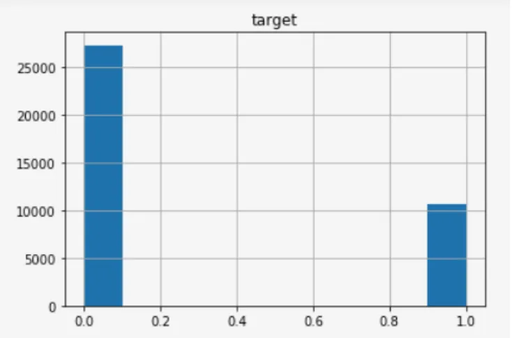
Figure 2 - Curator-defined target. On axis 0 we have the class and on axis 1 we have the number of observations

27

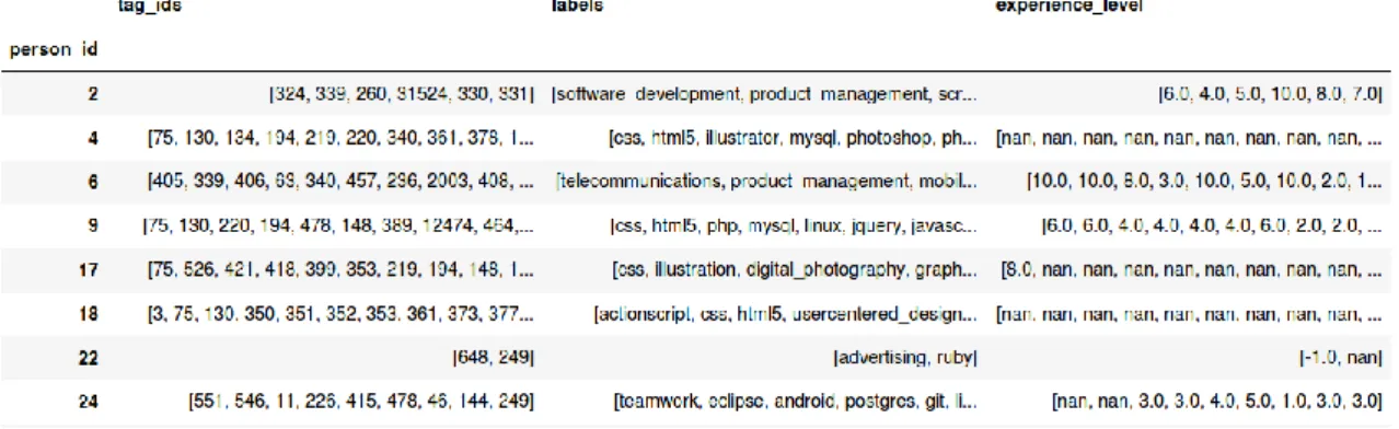
2.1. Extracting people skills and tags

Table ‘Skills’ holds the mapping between people and tags. A person has many skills and a skill can have many tags. Tags are text (skills name) and each one is unique in the database. However, the application has an engine which determines that when different tags possibly represent the same skill, then the skill points to a list of ‘tag_ids’ instead of a single ‘tag_id’. To the output of this engine is called ‘canonicalized skills’.

For each applicant, we are interested in joining in the same table, skill-ids, skills-name(tags) and experience per skills.

Brief summary of the transformations applied:

1) We are only interested in skills of people whose applications are part of out target dataset, so we start by filtering the ‘Skills’ table retaining only those of people in our target table.

2) Now we will work on the ‘canonicalized_tag_ids’ column. First we remove ‘{ }’ from all the rows. Then, we convert the string of tag ids into a list. String with multiple tag ids will return a list with multiple indices. Finally, we convert column data to integers.

Table 2 - canonicalized tags ids transformed Table 1 - Skills table

28 3) Now we breakdown the rows where skills have multiple tags into new rows and use a second level index to keep track of those rows whose skill ids are now duplicated. We have our skills dataframe ready.

4) Import ‘Tags’ table.

Table 4 - Tags table

5) We execute a left join between skills and tags dataframe, using ‘tag_id’ as key, resulting a new dataframe called ‘skillTags’.

6) For last, we group ‘skillTags dataframe by person_id concatenating in a single list all the values of a certain field related with the same person. The fields we are interested are ‘tag_ids’, ‘label’ and ‘experience’.

29

3. Job ad features – create job ads dataset

To build a dataset representing the attribute of a job ad, we need to pick attributes from tables ‘JobAds’, ‘Companies’ and ‘Tags’. A job ad has a company while a company can have multiple job ads. A job ad requires multiple skills and each skill has a label.

Table “JobAds” has considerable number of fields. We get rid of all system columns as well as fields related with bureaucracy associated with the job ad.

From the remaining fields, we break them down into 7 groups, each one corresponding to a different perspective on the job ad based on our judgement. In any case, the purpose was merely to start having some hints on which feature could be used or built for the Machine Learning models that we will be later and to make the code more readable. Then, we merge jobAds table with Companies table.

Table 5 - Skill tags per person

30

3.1. Extracting required skills and nice-to-have skills

Job ads specify the required skills for the job and the additional or nice-to-have skills. These information is presented in the table ‘job ads’ in the fields ‘extracted_main_skill_ids’ and ‘extracted_additiona_skill_ids’. These fields come in the form showing in table 15. Please note that the ids of both of these fields point to Tag ids and not to Skills ids, contrary to what the name suggests.

Our goal is to obtain the list of required and nice-to-have skills per job ad and the corresponding labels. To do so, for both fields, we apply most of the same transformation that we briefed in section 2.1, which include:

1) Converting string of ids to list of integers;

2) Break down each list into the corresponding number of rows; 3) Merge with table Tags to get the labels.

G. Experiments

We divide logically the experiments conducted into two groups. The techniques applied in both are highly intersected, however in experiment set A, we use a simple TF-IDF (Term Frequency-Inverse of Document Frequency)1 _{approach to convert job and applicants’ skills into a}

1 _{Term-frequency matrix is a tabular representation of data where documents are usually assigned to the}

rows and the collection of terms through all documents are represented as columns. The values of the Table 6 - Job ad skills

31 document matrix and apply the cosine similarity on the applicant skills vector and job skills vector. In experiment set B, we test a set of different NLP techniques to further improve the ability to match the skills of the applicant with those required in the job ad. In experiment B, apart from the Skills-matching re-estimation, we rely on the same data-preprocessing techniques and features (except skills-matching) applied in experiment set A to generate the final dataset for training.

Experiment-set A

Feature engineering

In this section we introduce the features we generate to serve as input for the Machine Learning algorithms we apply later. The set of features we generate can be split into two groups: the matching group and the descriptive group. The matching group refers to the set of features generated in order to allow a comparison of similar dimensions between the job requirements and the candidate profile, for instance the matching between the skills required and the skills presented in the candidate’s profile. The descriptive group are features for which either was not possible to draw a match or are purely one-sided features. One example of the former is where candidates present their experience years as a continuous variable, while the job postings state the required experience level as a category representing ranges of years of experience. For the latter case an example is whether Landing.Jobs considered the company offering the job position as strategic or not strategic.

1. Skills-matching

Let 𝐴 be the set of all applications in our data 𝐷 and 𝐴𝑛 be the 𝑛𝑡ℎ application.

Let R be the set of all skills required in the job ad and O be the set of all skills offered by the applicants.

Skills are represented as a vector of strings encoded as a TF-IDF matrix. Each application 𝐴𝑛 contains a job ad 𝑗 and a person/applicant 𝑝.

The skills-matching coefficient is the similarity between the vector of skills required 𝑅𝑗 in the job ad 𝑗 and the vector of skills offered 𝑂𝑝 by the applicant 𝑝.

Let:

𝐾 = 𝑅 ∪ 𝑂 representing the union of all skills vector into a single set.

To encode the vectors of skills, we transform 𝐾 into a TF-IDF sparse matrix 𝐾. In text-mining terms, we implicitly consider each vector of skills a document and each skill a term.

The similarity measure used is the commonly applied cosine-similarity.

matrix represent the frequency each term appears per document. Usually it is multiplied by the inverse of the frequency of the term in the documents so as to give less important to terms which are very common and appear in most documents while stressing the importance of less common terms. In this case, the matrix is called Term-Frequency Inverse of Document Frequency (TF-IDF) matrix.

32 Therefore, the similarity 𝑆𝑛 computed for each pair ( 𝑅𝑗 , 𝑂𝑝 ) comes as:

𝑆𝑛= cosine ( 𝑅𝑗 , 𝑂𝑝 ) ∈ 𝐴𝑛, ∀ 𝑛 = 1, 2 … 𝑁, where 𝑁 is the total number of applications in the data.

2. Profession-matching

Professional-matching represents how well the person’s professional title, denoted in our data as the headline, matches with the name of the job role. The first impression a person conveys in her headline when compared with the name of the job role, might provide some insights on the degree of matching between a candidate and a job position.

We start by considering candidate’s professional title and name of job role as strings and the first metric we extract is the distance between those string. For that we use Levenshtein distance metric which counts the number of character edits needed in one strings for it to become like the other one (Navarro, 2001). While Levenshtein distance metric is intuitive and easy to understand, we acknowledge some shortcomings such as ignoring the semantics of words. For instance, headline ‘Experienced Software Developer’ would match highly with job role ‘Software Developer’, however ‘Front-end Developer’ matches very poorly with ‘UI Engineer, even though one can consider that the two strings are semantically connected.

Let’s use the same notation as in the skills-matching, where, in this profession-matching context, 𝑅𝑗 is name of job role presented on job ad 𝑗 and 𝑂𝑝 is the applicant 𝑝 headline.

Therefore, the distance 𝑆𝑛 computed for each pair (𝑅𝑗, 𝑂𝑝) comes as:

𝑆𝑛 = levenshtein (𝑅𝑗, 𝑂𝑝) ∈ 𝐴𝑛, ∀ 𝑛 = 1, 2 … 𝑁

The final match value is computed by dividing the distance 𝑆𝑛 by the length of the longest of the two strings.

3. Location-matching

Location-matching intends to find the degree of matching between the applicant location or a location the applicant considers moving to and the job location. As an illustration for the pertinence of this feature consider that a candidate from a certain country applies for a job in another country for which a visa is required but the recruiter company is not sponsoring the visa application. As briefed by a Landing.Job official and through our domain knowledge, we suspect that these applicants would be in a less favorable situation and that this may be embedded in the selection criteria.

33 The following variables were defined before estimating the location-matching coefficient. Let 𝐶 represent the country-matching, then:

𝐶 = {1 𝑖𝑓 𝑡ℎ𝑒 𝑎𝑝𝑝𝑙𝑖𝑐𝑎𝑛𝑡 𝑖𝑠 𝑓𝑟𝑜𝑚 𝑡ℎ𝑒 𝑠𝑎𝑚𝑒 𝑐𝑜𝑢𝑛𝑡𝑟𝑦 𝑎𝑠 𝑡ℎ𝑒 𝑗𝑜𝑏 0 𝑜𝑡ℎ𝑒𝑟𝑤𝑖𝑠𝑒

Let 𝐿 represent the relocation-matching, then:

𝐿 = {1 𝑖𝑓 𝑗𝑜𝑏 𝑙𝑜𝑐𝑎𝑡𝑖𝑜𝑛 𝑖𝑠 𝑖𝑛 𝑡ℎ𝑒 𝑟𝑒𝑙𝑜𝑐𝑎𝑡𝑖𝑜𝑛 𝑐𝑜𝑢𝑛𝑡𝑟𝑖𝑒𝑠 𝑙𝑖𝑠𝑡 𝑜𝑓 𝑡ℎ𝑒 𝑎𝑝𝑝𝑙𝑖𝑐𝑎𝑛𝑡 0 𝑜𝑡ℎ𝑒𝑟𝑤𝑖𝑠𝑒

Let 𝑉 represent the visa-matching, then:

𝑉 = { 1 𝑖𝑓 𝑣𝑖𝑠𝑎 𝑠𝑢𝑝𝑝𝑜𝑟𝑡 𝑎𝑛𝑑 𝑟𝑒𝑙𝑜𝑐𝑎𝑡𝑖𝑜𝑛 𝑝𝑎𝑖𝑑, 0.5 𝑖𝑓 𝑣𝑖𝑠𝑎 𝑠𝑢𝑝𝑝𝑜𝑟𝑡 𝑜𝑟 𝑟𝑒𝑙𝑜𝑐𝑎𝑡𝑖𝑜𝑛 𝑝𝑎𝑖𝑑, 0 𝑖𝑓 𝑛𝑜𝑡 𝑣𝑖𝑠𝑎 𝑠𝑢𝑝𝑝𝑜𝑟𝑡 𝑛𝑜𝑟 𝑟𝑒𝑙𝑜𝑐𝑎𝑡𝑖𝑜𝑛 𝑝𝑎𝑖𝑑

Let 𝑅 represent the remote-matching, then:

𝑅 = { 1 𝑖𝑓 𝑓𝑢𝑙𝑙 𝑟𝑒𝑚𝑜𝑡𝑒 𝑗𝑜𝑏, 0.5 𝑖𝑓 𝑝𝑎𝑟𝑡𝑖𝑎𝑙 𝑟𝑒𝑚𝑜𝑡𝑒 𝑜𝑟 𝑊𝐹𝐻2 𝑜𝑟 𝑓𝑢𝑙𝑙 𝑟𝑒𝑚𝑜𝑡𝑒 𝑐𝑜𝑚𝑚𝑢𝑡𝑎𝑏𝑙𝑒, 0 𝑖𝑓 𝑛𝑜𝑡 𝑟𝑒𝑚𝑜𝑡𝑒

We then compute the location-match coefficient by applying a weight vector to C, L, V and R Let’s represent 𝐶, 𝐿, 𝑉 and 𝑅 as a vector 𝑙⃗. We use our domain knowledge to create a vector of weights as

𝑤⃗⃗⃗ = (0.3, 0.3, 0.25, 0.15)

Recall from the previous notation that 𝑝 be the applicant, 𝑗 the job ad and (𝑝, 𝑗) ∈ 𝐴𝑛, where 𝐴𝑛 is the 𝑛𝑡ℎ application.

Hence, the location-match coefficient comes as:

𝐿𝑜𝑐𝑀𝑎𝑡𝑐ℎ𝑛= 𝑙⃗⃗⃗⃗ · 𝑤𝑛 ⃗⃗⃗⃗⃗⃗ 𝑛

Other feature-matchings were considered, for instance, Salary-matching and Experience-matching. However, in the former case, most of the people don’t specify their salary expectation

34 nor is used a consistent scale used (e.g. units or thousands) and in the latter case, the experience required in the job ad is presented as classes with a non-homogenous scale (eg. Class 3 corresponds to 5 years of experience and class 4 corresponds to 7+ years of experience including leading).For the presented reasons, we decide to introduce salary and experience features in our feature set but we do not create a matching feature ourselves.

In the following, we present a set of descriptive features we generate to complement the aforementioned ones.

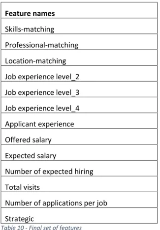
4. Additional features

Job experience level - Categorical

Job experience required in the job ad, converted to four dummy variables. Applicant experience - Continuous

Years of experience of the applicant. Strategic – Categorical / Boolean

Is a flag which encodes whether the company recruiting is strategic. Premium – Categorical / Boolean

Is a flag which encodes whether the job ad is premium. Perceived Commitment - Categorical

Represents the commitment of the recruiting company as perceived by the account manager. Three categories, converted to dummy variables.

Availability – Categorical

Encodes whether the applicant availability to start on the job, were she selected. Offered salary – Continuous

Salary offered for the job. Is truncated with a lower bound of 10.000 and a higher bound of 150.000. Null values are imputed using the intra-class mean salary for classes country, role and experience.

Expected salary – Continuous

Salary expected by the applicant. Is truncated with a lower bound of 10.000 and a higher bound of 150.000. Null values are imputed using the intra-class mean salary for classes country and experience.

Number of applications per job – Continuous Self-explanatory.

Number of expected hiring – Continuous

Number of people the company is recruiting for that job. Total visits – Continuous

35 Fee percentage – Continuous

Represents the price the recruiting company is paying to the Marketplace for their work.

Data preprocessing and feature selection

We begin our preprocessing phase by testing multicollinearity. Then we scale continuous features and applied a filtering algorithm.

For multicollinearity testing we used the VIF (variance inflation filter) algorithm as explained in Technical Background section. We suspected that our data could contain a high level of multicollinearity because whenever we transformed a categorical variable into dummy variables, we did not remove one of the dummies which should be considered the baseline dummy variable. In table 8 we can find the multicollinearity measurement scores where all features were considered and in table 9 we made available the multicollinearity measurement scores where we have removed a baseline class per categorical feature. The results are significantly different, with the latter set of features resulting in much lower scores. Though in the latter case some features show a VIF score over 20, we have considered the results acceptable, as there is not a consensus in the literature in regards to the acceptable values for the higher bound VIF score but these scores could be considered within an acceptable range (Dumancas & Ghalib, 2015).

Variable VIF type

jobExperLvl_1 5.035 categorical jobExperLvl_2 605 categorical jobExperLvl_3 25.146.274 categorical jobExperLvl_4 1.925.703.577 categorical is_strategic_job_0 34 categorical is_strategic_job_1 21.609 categorical premium_job_0 5.080 categorical premium_job_1 346 categorical perceived_commitment_jobAds_0 184.941.364.079 categorical perceived_commitment_jobAds_1 32 categorical perceived_commitment_jobAds_2 5.058.016.391 categorical availability_ppl_0 13.350.010 categorical availability_ppl_1 2.519.106 categorical availability_ppl_2 379 categorical availability_ppl_3 7.758 categorical skillsMatch 2 interval pplExperience 6 interval professionMatch 7 interval offeredSalary 7 interval expectedSalary 7 interval