A comparison of four data selection methods for artificial neural networks and support vector machines

(1)

IFAC PapersOnLine 50-1 (2017) 11227–11232

ScienceDirect

10.1016/j.ifacol.2017.08.1577

A Comparison of Four Data Selection Methods for Artificial Neural Networks

and Support Vector Machines

H. Khosravani*. A. Ruano*1_{, P. M. Ferreira **}



*Faculty of Science and Technology, University of Algarve, Faro, Portugal and IDMEC, Instituto Superior Técnico, Universidade de Lisboa, Lisboa, Portugal (e-mail: hkhosravani@csi.fct.ualg.pt, aruano@ualg.pt). **LaSIGE, Faculdade de Ciências, Universidade de Lisboa, Portugal (e-mail: pmf@ciencias.ulisboa.pt)}

Abstract: The performance of data-driven models such as Artificial Neural Networks and Support Vector Machines relies to a good extent on selecting proper data throughout the design phase. This paper addresses a comparison of four unsupervised data selection methods including random, convex hull based, entropy based and a hybrid data selection method. These methods were evaluated on eight benchmarks in classification and regression problems. For classification, Support Vector Machines were used, while for the regression problems, Multi-Layer Perceptrons were employed. Additionally, for each problem type, a non-dominated set of Radial Basis Functions Neural Networks were designed, benefiting from a Multi Objective Genetic Algorithm. The simulation results showed that the convex hull based method and the hybrid method involving convex hull and entropy, obtain better performance than the other methods, and that MOGA designed RBFNNs always perform better than the other models.

Keywords: Artificial Neural Networks, Convex Hull Algorithms, Entropy, Multi Objective Genetic Algorithm, Support Vector Machines



1_{The author would like to acknowledge the support of FCT through IDMEC, under LAETA grant UID/EMS/50022/2013.}

1. INTRODUCTION

In many machine learning and data mining problems two basic tasks have to be considered: feature selection and instance selection. The former denotes choosing a subset of all available features so that the selected subset has the strongest relation to the model output and yields improved model performance. The latter refers to sample selection where we are interested in selecting a subset of informative data samples (denoted by S) among all existing ones (denoted by D). The goal is that the model designed using S can maintain or even exceed the performance level (for instance, accuracy) that would be attained by using D. The instance selection process not only helps decreasing the run time of the training process but also has the benefit of reducing memory requirements. This is important when classification or regression tasks rely on existing large-size datasets. Instance selection methods can be classified into wrapper and filter methods. Wrapper methods use a model as a selection criterion, where the performance of the model is evaluated based on a subset of samples, iteration by iteration, to select those samples which have the most contribution on the model accuracy. Most works found in the literature on the wrapper or supervised methods relate to classification tasks. Some important contributions can be seen in (Cano, Herrera, & Lozano, 2003; Hart, 1968; Olvera-Lopez, Martinez-Trinidad, & Carrasco-Ochoa, 2007).

Unlike wrapper methods, filter or unsupervised methods employ a model independent selection function to choose

informative samples. This means that the accuracy of the model does not have any contribution in the selection criterion; instead, a selection rule is applied. Related works can be seen in (Pedro M. Ferreira, 2016; Khosravani, Ruano, & Ferreira, 2016; Paredes & Vidal, 2000).

Although comparison between Multi Objective Genetic Algorithm (MOGA) designed models and Multi-Layer Perceptrons (MLPs) and Support Vector Machines (SVMs) will take place, the main objective of this paper is to analyse the performance of four data selection methods, including Random Data Selection (RDS), Convex Hull Based Data Selection (CBDS), Entropy Based Data Selection (EBDS) and a Hybrid Data Selection (HDS) method. Among these methods, the CBDS and EBDS methods are previous efforts of the authors, presented in (Khosravani, et al., 2016) and (Pedro M. Ferreira, 2016), respectively, while the HDS method, a combination of CBDS and EBDS methods, is proposed in this paper as a new data selection method. The four methods data selection methods were applied on eight benchmarks related to classification and regression problems, employing SVMs and MLPs, respectively. For one problem of each type, MOGA, as a design platform (P. Ferreira & Ruano, 2011) was employed to additionally produce a non-dominated set of Radial Basis Function Neural Networks (RBFNN).

The rest of the paper is organized as follows: Section 2 introduces MOGA. The four data selection methods are explained in Section 3. The experiments and their Toulouse, France, July 9-14, 2017

11719

A Comparison of Four Data Selection Methods for Artificial Neural Networks

and Support Vector Machines



1. INTRODUCTION

The rest of the paper is organized as follows: Section 2 introduces MOGA. The four data selection methods are explained in Section 3. The experiments and their

A Comparison of Four Data Selection Methods for Artificial Neural Networks

and Support Vector Machines



1. INTRODUCTION

A Comparison of Four Data Selection Methods for Artificial Neural Networks

and Support Vector Machines



1

The author would like to acknowledge the support of FCT through IDMEC, under LAETA grant UID/EMS/50022/2013.

1. INTRODUCTION

(2)

corresponding simulation results are discussed in Section 4 and 5, respectively. Conclusions are given in Section 6.

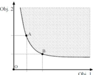
2. MULTI OBJSECTIVE GENETIC ALGORITHM In the real world, the optimization of an engineering problem is a complicated task due to the presence of multiple objectives which, most of time, are conflicting with each other. In this case, the solution is a Pareto-optimal or non-dominated set, where each solution is not better than the other with respect to the multiple objectives. Fig. 1 shows an example of a minimization problem with two objectives. The whole space of solutions is divided into two groups: the shaded region presents the dominated solutions while the solid curve illustrates the non-dominated set of solutions regarding objectives Obj.1 and Obj.2. As it can be seen in Fig.1, A and B denote two non-dominated solutions.

Fig. 1. Bi-objective minimization problem.

The goal of a multi-objective optimizer is to improve the approximation of the Pareto front (i.e. the solid curve) in such a way that it approaches the origin (i.e., point ‘O’ in Figure 1) as much as possible.

Genetic Algorithms are meta-heuristics often used for multi-objective optimization problems (Carlos M. Fonseca & Fleming, 1995). In MOGA, each individual in the population is evaluated in the space of the multiple objectives rather than in one objective, and is ranked based on the number of individuals by which it is dominated, using a Pareto-based ranking method proposed in (C. M. Fonseca & Fleming, 1998).

2.1. Neural network based model design by MOGA

The problem of designing a neural network model, based on training, testing and validation sets, can be considered from two points of view: structure selection and parameters estimation. In the aspect of structure, the network inputs and the number of hidden layers/neurons should be determined while, with respect to the network parameters, they should be adjusted using a proper training algorithm.

In this study RBFNN models are considered, which implies that the network parameters include the linear output weights (w) and the nonlinear parameters, the centres (C) and the spreads (σ_{) of the hidden neurons. In this study, MOGA}

was customized to design RBFNN models as follows: Assume that D denotes the whole dataset available for model design. Suppose that the training, generalization or testing and the validation sets are denoted as T, G and V, respectively. Assuming that we want models with input features in the range [dm,dM] and number of hidden neurons

in the range [n n_m, _M], MOGA will search that space, forming a non-dominated set of models according to the objectives specified, which can be minimized, or set as restrictions with possible different priorities. Typically, the objectives considered belong to [ _p, _s], where pand sdenote the

set of objectives related to the RBFNNs’ performance and their structure, respectively. In this work, s refers to the

model complexity, which is equal to the number of input features + 1, multiplied by the number of hidden neurons. For regression problems, pis defined as (1):

[ ( ), ( )]

p

   T  G (1)

where  T( ) and  G( ) denote the Root Mean Square Error (RMSE) of T and G, respectively. Regarding classification problems, _pis defined as (2):

[ ( ), ( ), ( ), ( )]

p FP FN FP FN

  T T G G (2)

WhereFP(.)and FN(.)denote the False Positives (FP) and the False Negatives (FN) obtained on the corresponding dataset, respectively. Each individual in the population has a chromosome representation consisting of two components. The first corresponds to the number of hidden neurons, and the second is a string of integers, each one representing the index of a particular feature, out of the ones allowed.

Before being evaluated in MOGA, each model has its parameters determined by a Levenberg-Marquardt (LM) algorithm (Levenberg, 1944) minimizing an error criterion that exploits the linear-nonlinear relationship of the RBFNN model parameters (P. M. Ferreira, Ruano, & Ieee, 2000; Ruano, Jones, & Fleming, 1991) . The initial values of the nonlinear parameters (C and

σ

_{) are chosen randomly, or}

with the use of a clustering algorithm, w is determined as a linear least-squares solution, and the procedure is terminated using the early-stopping (Haykin, 1999) within a maximum number of iterations. For more details of MOGA, please see (P. Ferreira & Ruano, 2011).

3. THE FOUR FILTER DATA SELECTION METHODS In this work, our goal is to extract, from the existing whole dataset D of size N by d (denoting the number of samples and the dimension, respectively.), three sub-datasets, T, G and V, containing Nt, Ng and Nv samples, respectively, in such a way

that T hopefully contains informative samples, which can result in models with a high level of performance. Since in this study, our goal is not necessarily data reduction, the data selection term is used instead of instance selection, throughout the rest of the paper. The following addresses the four data selection methods employed.

3.1. Random data selection method

The simplest way to partition D into T, G and V is using the RDS method. In this method, firstly, Nt samples are extracted

randomly from D (resulting in a reduced set D’) to construct

T. Subsequently, Ng samples are randomly extracted from D’

(resulting in a reduced set D’’) to form G and finally Nv

(3)

3.2. Convex hull based data selection method

To design data driven models like RBFNNs, it is very important that the training set involves the samples that represent the whole input-output range where the underlying process is supposed to operate. To determine such samples, called convex hull points, out of the whole dataset, convex hull algorithms can be applied. The standard convex hull algorithms suffer from both exaggerated time and space complexity in high dimensions. To tackle these challenges in high dimensions, ApproxHull was proposed in (Khosravani, et al., 2016) as a randomized approximation convex hull algorithm. To identify the convex hull points, ApproxHull employs two main computational geometry concepts; the hyperplane distance and the convex hull distance.

Given the point [ ,1 2,..., ] T d

v v v



v in a d-dimensional

Euclidean space and a hyperplane H, the hyperplane distance of v to H is obtained by (3): 1 1 2 2 2 2 2 1 2 ... ( , ) ... d d d a v a v a v b ds H a a a         v (3)

Where n



a a₁, ₂,...,a_d



Tand b are the normal vector and the offset of H , respectively. Given a set { } 1 n d i i     X x and a point _d x , the

Euclidean distance between x and the convex hull of X, denoted by conv(X), can be computed by solving the quadratic optimization problem stated in (4).

1 2 . . 1, 0

min

T T T s t  _        a a Qa c a e a a (4) where_e_[1,1,...,1]T ,_Q__{X X}T and _ T

c X x Suppose that the optimal solution of (4) is *

a ; then the distance of point x to conv(X) is given by (5):

* * *

( , ( )) T 2 T T

dc x conv X  x x c a a Qa (5) ApproxHull consists of five main steps. In Step 1, each dimension of the input dataset is scaled to the range [-1, 1]. In Step 2, the maximum and minimum samples with respect to each dimension are identified and considered as the vertices of the initial convex hull. In Step 3, a population of k facets based on the current vertices of the convex hull is generated. In Step 4, the furthest points to each facet in the current population are identified using (3) and they are considered as the new vertices of the convex hull, if they have not been detected before. Finally, in Step 5, the current convex hull is updated by adding the newly found vertices into the current set of vertices. Step 3 to Step 5 are executed iteratively until no vertex found in Step 4 or the newly found vertices are very close to the current convex hull, thus not containing useful information. The closest points to the current convex hull are identified using the convex hull distance shown in (5) and a user-defined threshold.

In the CBDS method, first ApproxHull is applied on the dataset D to obtain the convex hull points (the vertices of the approximated convex hull). Afterwards, the convex hull points as well as some random samples are extracted from D

to form T. These are removed from D, forming D’. The G and V sets are obtained as in the RDS method.

3.3. Entropy based data selection method

As a recent effort in filter data selection domain, an Entropy Based Data Selection method was proposed in (Pedro M. Ferreira, 2016). The main idea behind the EBDS method is selecting Nt samples of D to form the training set T so that

the information content and the diversity of data in T used to adjust the model parameters is maximized. This method employs the information entropy of any random variable Z given in (6). ( ) ( ) ( ) 1 N H p z I z i i i    Z (6)

Where N is the number of all possible observations of Z.

 

i

p z _{denotes the probability that Z takes the value}z_i(the ith

sample in D) and I z

 

i denotes the information content that

Z represents when it takes value z_i. I z

 

is defined as (7).

( ) 2

( ) logp z

I z   (7)

Since dataset D represents a set of values of a multidimensional random variable, p z

 

i is translated into

the probability that Z takes the valuezi In this method, p z( )i

is estimated by (8). 1 1 1 1 ˆ ( ) [ ( [ ] [ ])] l d N i h i j j i p z k z l z l N    

 

 (8) where

 

. l h

k is a Gaussian kernel function whose bandwidth is hl, obtained by (9): 1 ( 1 4) ˆ d l l h



N     (9)

where ˆ_l is the sample standard deviation along dimension l of the data. Based on the above, the EBDS method works as follows: In the first step, vector ˆpis obtained as (10) using (8) for each sample in zi in D.

1 2

ˆ [ ( ), ( ),..., (p zˆ p zˆ p zˆ N)]

p (10)

In the second step, vector ˆIis obtained as (11) using (7) for each sample ziin D. 1 2 ˆ _{[ ( ), ( ),..., (}ˆ ˆ ˆ _)] N I z I z I z  I (11)

Having ˆp and ˆI at hand, vector H is obtained as (12) by taking the Hadamard product of ˆp by ˆI.

1 1 2 2 ˆ _{[ ( ) ( ), ( ) ( ),..., (}_ˆ ˆ _ˆ ˆ _ˆ _{) (}ˆ _)] N N p z I z p z I z p z I z  H (12)

where p z I zˆ ( ) ( )i ˆ i is considered as the information based

fitness of sample zi, reflecting the contribution of sample zi

to the entropy obtained by (6). Once vector Hˆ is obtained, Nt

samples are removed from D using the Stochastic Universal Sampling method (Baker, 1987), to form T. The other two sets are obtained as in the RDS.

3.4. Hybrid data selection method corresponding simulation results are discussed in Section 4

and 5, respectively. Conclusions are given in Section 6. 2. MULTI OBJSECTIVE GENETIC ALGORITHM In the real world, the optimization of an engineering problem is a complicated task due to the presence of multiple objectives which, most of time, are conflicting with each other. In this case, the solution is a Pareto-optimal or non-dominated set, where each solution is not better than the other with respect to the multiple objectives. Fig. 1 shows an example of a minimization problem with two objectives. The whole space of solutions is divided into two groups: the shaded region presents the dominated solutions while the solid curve illustrates the non-dominated set of solutions regarding objectives Obj.1 and Obj.2. As it can be seen in Fig.1, A and B denote two non-dominated solutions.

Fig. 1. Bi-objective minimization problem.

The goal of a multi-objective optimizer is to improve the approximation of the Pareto front (i.e. the solid curve) in such a way that it approaches the origin (i.e., point ‘O’ in Figure 1) as much as possible.

Genetic Algorithms are meta-heuristics often used for multi-objective optimization problems (Carlos M. Fonseca & Fleming, 1995). In MOGA, each individual in the population is evaluated in the space of the multiple objectives rather than in one objective, and is ranked based on the number of individuals by which it is dominated, using a Pareto-based ranking method proposed in (C. M. Fonseca & Fleming, 1998).

2.1. Neural network based model design by MOGA

The problem of designing a neural network model, based on training, testing and validation sets, can be considered from two points of view: structure selection and parameters estimation. In the aspect of structure, the network inputs and the number of hidden layers/neurons should be determined while, with respect to the network parameters, they should be adjusted using a proper training algorithm.

In this study RBFNN models are considered, which implies that the network parameters include the linear output weights (w) and the nonlinear parameters, the centres (C) and the spreads (σ_{) of the hidden neurons. In this study, MOGA}

was customized to design RBFNN models as follows: Assume that D denotes the whole dataset available for model design. Suppose that the training, generalization or testing and the validation sets are denoted as T, G and V, respectively. Assuming that we want models with input features in the range [dm,dM] and number of hidden neurons

in the range [n n_m, _M], MOGA will search that space, forming a non-dominated set of models according to the objectives specified, which can be minimized, or set as restrictions with possible different priorities. Typically, the objectives considered belong to [ _p, _s], where pand sdenote the

set of objectives related to the RBFNNs’ performance and their structure, respectively. In this work, s refers to the

model complexity, which is equal to the number of input features + 1, multiplied by the number of hidden neurons. For regression problems, pis defined as (1):

[ ( ), ( )]

p

   T  G (1)

where  T( ) and  G( ) denote the Root Mean Square Error (RMSE) of T and G, respectively. Regarding classification problems, _pis defined as (2):

[ ( ), ( ), ( ), ( )]

p FP FN FP FN

  T T G G (2)

WhereFP(.)and FN(.)denote the False Positives (FP) and the False Negatives (FN) obtained on the corresponding dataset, respectively. Each individual in the population has a chromosome representation consisting of two components. The first corresponds to the number of hidden neurons, and the second is a string of integers, each one representing the index of a particular feature, out of the ones allowed.

Before being evaluated in MOGA, each model has its parameters determined by a Levenberg-Marquardt (LM) algorithm (Levenberg, 1944) minimizing an error criterion that exploits the linear-nonlinear relationship of the RBFNN model parameters (P. M. Ferreira, Ruano, & Ieee, 2000; Ruano, Jones, & Fleming, 1991) . The initial values of the nonlinear parameters (C and

σ

_{) are chosen randomly, or}

with the use of a clustering algorithm, w is determined as a linear least-squares solution, and the procedure is terminated using the early-stopping (Haykin, 1999) within a maximum number of iterations. For more details of MOGA, please see (P. Ferreira & Ruano, 2011).

3. THE FOUR FILTER DATA SELECTION METHODS In this work, our goal is to extract, from the existing whole dataset D of size N by d (denoting the number of samples and the dimension, respectively.), three sub-datasets, T, G and V, containing Nt, Ng and Nv samples, respectively, in such a way

that T hopefully contains informative samples, which can result in models with a high level of performance. Since in this study, our goal is not necessarily data reduction, the data selection term is used instead of instance selection, throughout the rest of the paper. The following addresses the four data selection methods employed.

3.1. Random data selection method

The simplest way to partition D into T, G and V is using the RDS method. In this method, firstly, Nt samples are extracted

randomly from D (resulting in a reduced set D’) to construct

T. Subsequently, Ng samples are randomly extracted from D’

(resulting in a reduced set D’’) to form G and finally Nv

(4)

The idea behind the Hybrid Data Selection method is combining the two previous methods, CBDS and EBDS. In the first step of HDS method, ApproxHull is applied on D to extract the corresponding convex hull points (resulting in a reduced set D’) and included in T. Suppose that the number of convex hull points is denoted as Nch. In the next step, Nt -

Nch samples are extracted from D’ using the EBDS method

and included in T. G and V are obtained from the rest of the samples in the same way as in the RDS method.

4. EXPERIMENTS

To evaluate the performance of the data selection methods, 8 benchmarks were considered: 4 binary class classification problems, and the others related to regression. For one regression problem (Bank) and one classification problem (Breast Cancer), three type of models are considered. For the other benchmarks, only one model type will be considered. Each model type involves four experiments, each one corresponding to a data selection method.

For RBFNN MOGA models, two scenarios will be considered. As in the end of each MOGA, we have access to a set of non-dominated models, typically we must choose one model out of this set. This scenario will be called best model. The criterion for selecting the best model out of the set of MOGA non-dominated models for the regression problem is the minimum RMSE on the common validation set V.





/

CR TP TN N (13)

Denoting as CR the Classification Rate defined in (13), the best model for the classification problem will be determined in three steps: first, all models which have the maximum CR(V) are selected; from them, the ones with maximum CR(G) are chosen; finally, for the latter, the one with maximum CR(T) will be selected.

The second scenario, called ensemble, involves using all non-dominated solutions. In this scenario, for the regression problem, the output of the ensemble scheme is the average of all non-dominated models' outputs, whereas for the classification, the output of the ensemble scheme is determined based on the majority of all models' outputs in the non-dominated set.

The third group of problems uses different models. In the case of a regression problem (Bank), the two MOGA model types are also compared with MLPs, trained with the modified LM algorithm introduced in (P. M. Ferreira, et al., 2000; Ruano, et al., 1991), which will be applied for the other regression benchmarks problems. For the classification problems, SVM (Matlab implementation) models are employed. For the Breast Cancer problem, SVM models are also compared with RBFNN models. For MLPs and SVMs, 10 experiments were conducted, while for each MOGA model, due to its time complexity, 5 experiments were executed for Bank and 5 for Breast Cancer. For all models and experiments, the four data selection methods were used. The datasets were taken from the UCI repository (Frank & Asuncion, 2013). Their number of samples (N) and inputs (d) is given in Table 1.

To fairly compare the data selection methods, the existence

of a common validation dataset, V, which does not have any contribution in model design, is needed. Notice, however, that in a practical case, each data selection method should be applied to the whole dataset, D. This is particularly relevant for the methods relying in convex hull (CBDS and HDS methods), as their rational is incorporating in the training set the convex hull points obtained from the whole dataset.

Table 1. Size of datasets.

Problem N d

Bank Regression 8192 32

Puma Regression 8192 32

Concrete Regression 1030 8

Wine Quality Regression 4898 11

Breast Cancer Classification 569 30

Parkinson Classification 1040 26

Satellite Classification 2033 36

Letter Classification 1555 16

In this paper, as we aim to compare the performance of the data selection models in a common validation set, the procedures explained previously for constructing the datasets are slightly modified. First, a common validation set V for each experiment is randomly extracted from the whole dataset; the remaining samples will constitute set D, from where the sets T and G will be extracted, according to the procedures explained before. The number of samples of T, G,

V and the average number of convex hull points (Nch)

obtained in all experiments of each problem is given in Tbl 2.

Table 2. Number of samples of T, G and V and the average number of convex hull points.

Nt Ng Nv Nch Bank 4195 1638 1639 3437 Concrete 618 206 206 307 Puma 4915 1638 1639 3686 Wine Quality 3134 784 980 599 Breast Cancer 300 76 193 183 Parkinson 550 136 354 280 Satellite 1074 268 691 711 Letter 822 204 529 564

Regarding the MOGA’s formulation, for all experiments, early stopping with a maximum of 100 iterations was considered. The number of generations and the population size were both set to 100. For all experiments, no restriction on objectives was considered, i.e. for the regression problem the objectives in (1) are minimized, while for the classification problem, the objectives in (2) are minimized. The range of the number of neurons was set to [2, 30] for all experiments. The range of the number of features for Bank and Breast Cancer was set to [1, 32] and [1, 30], respectively. In terms of model structure, the MLP models with 2 hidden layers used all features as inputs. The number of neurons for each hidden layer for Bank and Puma, was 10, while for the others was 5. For all MLP models, a maximum of 100 training iterations was considered.

Regarding the SVM models for the binary class classification problems, for all experiments, all features were used. The

(5)

corresponding hyper parameters γ and C were set to 0.05 and 1, respectively.

5. SIMULATION RESULTS

For the regression problems, the average of RMSEs of the common dataset V over the experiments, for the two MOGA models and the MLP model is given in Table 3.

Table 3. Average RMSEs obtained for dataset Bank.

RDS CBDS EBDS HDS

Best model 0.1908 0.1901 0.1907 0.1903

Ensemble 0.1870 0.1872 0.1869 0.1878

MLP 0.1969 0.1963 0.1979 0.1963

As shown in Table 3, independently of the data selection method, MOGA models are always better than MLP models, despite the latter being much more complex. In fact, MLPs have a model complexity (number of nonlinear parameters) of 440 while, using the average number of input features and neurons shown in Table 4, we can estimate that MOGA models have a maximum complexity of 104. Another conclusion that can be taken from Table 3 is that ensemble models show better performance than best models.

Table 4. Average number of features and neurons of the best MOGA models for dataset Bank.

Method Number of features Number of neurons

RDS 24 4

CBDS 20 5

EBDS 25 4

HDS 25 4

Regarding all regression models with MLP models, Table 5 shows the averages RMSEs.

Table 5. Average RMSEs for the regression problems.

RDS CBDS EBDS HDS

Bank 0.1969 0.1963 0.1979 0.1963

Concrete 0.1408 0.1417 0.1458 0.1408

Puma 0.0687 0.0671 0.0676 0.0687

Wine Quality 0.2361 0.2349 0.2370 0.2370

Regarding the best data selection method, the bold values in Tables 3 and 5 denote the best performance, for each model type/problem. Although it seems to indicate that CBDS and HDS should be chosen as best, with a slightly advantage of the former, the average RMSEs might not be the only criterion for that selection.

To analyse the statistical validity of the results, two tests are used: a sign test, and a Wilcoxon signed-ranks test. For the former, we counted, for each problem or group of problems, the number of times (C) that a data selection method (say j) had a better performance than another method (i), for each model type. For the latter test, assume that dk is the difference

between the performance scores (RMSEs or Classification Rates) of two approaches on the kth_{out of N datasets. The}

differences are ranked according to their absolute values; average ranks are assigned in case of ties. Let R+_{be the sum}

of ranks for the datasets on which the second approach outperformed the first, and R−_{the sum of ranks for the}

opposite. Defining T as





min ,

T R R  , (14)

Tables 6 shows the C(i,j) and T values, considering the Best and the Ensemble RBFNN models, for dataset Bank.

Table 6.

C(i,j)

/T for Bank – best and ensemble models

C(i,j)/T RDS CBDS EBDS HDS

RDS 8/19 4/26.5 6/27

CBDS 2/19 4/21 4/20

EBDS 5/26.5 6/21 4/23

HDS 4/27 6/20 6/23

Analysing the results of Tables 3 and 5 shows the CBDS method is the best one. Statistically, however, according to the Wilcoxon test, no method can be considered better than the others, while according to the sign test (weaker than the Wilcoxon test), we can only say that CBDS outperforms RDS method, with a level of significance of 10%. Table 7 shows the C(i,j) and T values for the 40 MLP experiments.

Table 7.

C(i,j)

/T for all MLP models

RDS 25/307 17/308.5 22/386.5

CBDS 13/307 12/238.5 16/306

EBDS 23/308.5 27/238.5 24/305.5

HDS 18/386.5 23/306 15/305.5

Analysing this table, CBDS should also be the chosen data selection method, which has, according to both tests, statistical validity, with a level of significance of 5%.

Considering now the classification problems, the average CR values for dataset Breast Cancer are shown in Table 8.

Table 8. Average CRs for Breast Cancer.

RDS CBDS EBDS HDS

Best model 0.9762 0.9803 0.9762 0.9783

Ensemble 0.9689 0.9689 0.9700 0.9679

SVM models 0.9601 0.9668 0.9611 0.9653

As it can be seen, MOGA models achieve better performance than SVM models, despite the huge difference in complexity. The average number of features (#F) and neurons for the MOGA models (#N) as well as the average number of support vectors for SVMs (#S) are given in Table 9. We can say that the largest complexity of RBFNN MOGA models is 42, while the smallest complexity of SVMs is 4691.

Table 9. Average number of features, neurons of the best MOGA models, and support vectors, for Breast Cancer.

Method #F #N #S

RDS 8 3 159

CBDS 10 3 160

EBDS 13 3 156

HDS 6 3 159

In contrast with the results found for Bank, here the performance of the ensemble is inferior to the best model. Analysing the performance of the four data selection models in Tables 8 and 10, CBDS seems again to be the method to apply. In the same way as in the regression cases, Table 11 The idea behind the Hybrid Data Selection method is

combining the two previous methods, CBDS and EBDS. In the first step of HDS method, ApproxHull is applied on D to extract the corresponding convex hull points (resulting in a reduced set D’) and included in T. Suppose that the number of convex hull points is denoted as Nch. In the next step, Nt -

Nch samples are extracted from D’ using the EBDS method

and included in T. G and V are obtained from the rest of the samples in the same way as in the RDS method.

4. EXPERIMENTS

To evaluate the performance of the data selection methods, 8 benchmarks were considered: 4 binary class classification problems, and the others related to regression. For one regression problem (Bank) and one classification problem (Breast Cancer), three type of models are considered. For the other benchmarks, only one model type will be considered. Each model type involves four experiments, each one corresponding to a data selection method.

For RBFNN MOGA models, two scenarios will be considered. As in the end of each MOGA, we have access to a set of non-dominated models, typically we must choose one model out of this set. This scenario will be called best model. The criterion for selecting the best model out of the set of MOGA non-dominated models for the regression problem is the minimum RMSE on the common validation set V.





/

CR TP TN N (13)

Denoting as CR the Classification Rate defined in (13), the best model for the classification problem will be determined in three steps: first, all models which have the maximum CR(V) are selected; from them, the ones with maximum CR(G) are chosen; finally, for the latter, the one with maximum CR(T) will be selected.

The second scenario, called ensemble, involves using all non-dominated solutions. In this scenario, for the regression problem, the output of the ensemble scheme is the average of all non-dominated models' outputs, whereas for the classification, the output of the ensemble scheme is determined based on the majority of all models' outputs in the non-dominated set.

The third group of problems uses different models. In the case of a regression problem (Bank), the two MOGA model types are also compared with MLPs, trained with the modified LM algorithm introduced in (P. M. Ferreira, et al., 2000; Ruano, et al., 1991), which will be applied for the other regression benchmarks problems. For the classification problems, SVM (Matlab implementation) models are employed. For the Breast Cancer problem, SVM models are also compared with RBFNN models. For MLPs and SVMs, 10 experiments were conducted, while for each MOGA model, due to its time complexity, 5 experiments were executed for Bank and 5 for Breast Cancer. For all models and experiments, the four data selection methods were used. The datasets were taken from the UCI repository (Frank & Asuncion, 2013). Their number of samples (N) and inputs (d) is given in Table 1.

To fairly compare the data selection methods, the existence

of a common validation dataset, V, which does not have any contribution in model design, is needed. Notice, however, that in a practical case, each data selection method should be applied to the whole dataset, D. This is particularly relevant for the methods relying in convex hull (CBDS and HDS methods), as their rational is incorporating in the training set the convex hull points obtained from the whole dataset.

Table 1. Size of datasets.

Problem N d

Bank Regression 8192 32

Puma Regression 8192 32

Concrete Regression 1030 8

Wine Quality Regression 4898 11

Breast Cancer Classification 569 30

Parkinson Classification 1040 26

Satellite Classification 2033 36

Letter Classification 1555 16

In this paper, as we aim to compare the performance of the data selection models in a common validation set, the procedures explained previously for constructing the datasets are slightly modified. First, a common validation set V for each experiment is randomly extracted from the whole dataset; the remaining samples will constitute set D, from where the sets T and G will be extracted, according to the procedures explained before. The number of samples of T, G,

V and the average number of convex hull points (Nch)

obtained in all experiments of each problem is given in Tbl 2.

Table 2. Number of samples of T, G and V and the average number of convex hull points.

Nt Ng Nv Nch Bank 4195 1638 1639 3437 Concrete 618 206 206 307 Puma 4915 1638 1639 3686 Wine Quality 3134 784 980 599 Breast Cancer 300 76 193 183 Parkinson 550 136 354 280 Satellite 1074 268 691 711 Letter 822 204 529 564

Regarding the MOGA’s formulation, for all experiments, early stopping with a maximum of 100 iterations was considered. The number of generations and the population size were both set to 100. For all experiments, no restriction on objectives was considered, i.e. for the regression problem the objectives in (1) are minimized, while for the classification problem, the objectives in (2) are minimized. The range of the number of neurons was set to [2, 30] for all experiments. The range of the number of features for Bank and Breast Cancer was set to [1, 32] and [1, 30], respectively. In terms of model structure, the MLP models with 2 hidden layers used all features as inputs. The number of neurons for each hidden layer for Bank and Puma, was 10, while for the others was 5. For all MLP models, a maximum of 100 training iterations was considered.

Regarding the SVM models for the binary class classification problems, for all experiments, all features were used. The

(6)

illustrates the C(i,j) and T values for the MOGA models, and Table 12 for the all 40 SVM models.

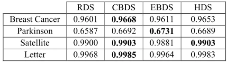
Table 10. Average CRs for the classification problems.

RDS CBDS EBDS HDS

Breast Cancer 0.9601 0.9668 0.9611 0.9653

Parkinson 0.6587 0.6692 0.6731 0.6689

Satellite 0.9900 0.9903 0.9881 0.9903

Letter 0.9968 0.9985 0.9964 0.9983

Table 11.

C(i,j)

/T for Breast Cancer – best and ensemble

RDS 4/14.5 3/25 3/19.5

CBDS 2/14.5 3/22.5 3/23

EBDS 4/25 4/22.5 5/25

HDS 3/19.5 5/23 4/25

In the case of MOGA models, the indication found in Tables 8 and 10 seems to be confirmed, although without statistical validity.

Table 12.

C(i,j)

/T for all SVM models

RDS 20/222.5 16/399.5 20/215

CBDS 8/222.5 9/251.5 9/391

EBDS 16/339.5 23/251.5 21/292

HDS 9/215 10/391.5 9/292

For the SVM models, we can say that, with a level of significance of 5%, CBDS is better than RDS and EBDS, and HDS is better than EBDS, according to the sign test.; based on the Wilcoxon test, HDS and CBDS are better than RDS, and HDS is better than EBDS. Using a level of significance of 10%, we have the union of both cases, with 5% level.

6. CONCLUSIONS

We have compared the performance obtained with MOGA designed models against MLPs (for regression) and SVMs (for classification). It was shown that MOGA models obtain much better performance, despite the much smaller complexity. Another conclusion that can be taken is that the naïve versions of the ensemble of non-dominated MOGA models proposed here, in some cases perform better, while in other cases worse than the selected best model.

In relation with the best data selection methods, we can say that the CBDS and HDS should be used, for SVM and MLP models. For the RBFNN MOGA models, the same conclusion can be taken, although without any statistical validity. This can be explained by the small number of experiments conducted, due to the high computational time, and also to the much better performance obtained by these models, compared with MLPs and SVMs, which reduces the range of differences between the data selection methods. Finally, it is expected that better performance can be achieved by the CBDS and HDS, when applied to the whole data; this is justified by comparing results obtained here with the results shown in (Khosravani, et al., 2016)

REFERENCES

Baker, J. E. (1987). Reducing bias and inefficiency in the selection algorithm. In: Proceedings of the Second International Conference on Genetic Algorithms (pp. 14-21), pp. 14-21.

Cano, J. R., Herrera, F., & Lozano, M. (2003). Using evolutionary algorithms as instance selection for data reduction in KDD: An experimental study. Ieee Transactions on Evolutionary Computation, 7 (6), 561-575.

Ferreira, P., & Ruano, A. (2011). Evolutionary Multiobjective Neural Network Models Identification: Evolving Task-Optimised Models. In: Ruano, A. & Várkonyi-Kóczy, A. (Eds.), New Advances in Intelligent Signal Processing (Vol. 372, pp. 21-53). Springer Berlin / Heidelberg, pp. 21-53.

Ferreira, P. M. (2016). Entropy Based Unsupervised Selection of Data Sets for Improved Model Fitting. In: Proceedings of the 2016 International Joint Conference on Neural Networks (World Congress on Computational Intelligence). IEEE, Vancouver, Canada.

Ferreira, P. M., Ruano, A. E., & Ieee, I. (2000). Exploiting the separability of linear and nonlinear parameters in radial basis function networks. Ieee 2000 Adaptive Systems for Signal Processing, Communications, and Control Symposium - Proceedings, 321-326.

Fonseca, C. M., & Fleming, P. J. (1995). An Overview of Evolutionary Algorithms in Multiobjective Optimization. Evolutionary Computation, 3 (1), 1-16.

Fonseca, C. M., & Fleming, P. J. (1998). Multiobjective optimization and multiple constraint handling with evolutionary algorithms. I. A unified formulation. Systems, Man and Cybernetics, Part A: Systems and Humans, IEEE Transactions on, 28 (1), 26-37.

Frank, A., & Asuncion, A. (2013). UCI Machine Learning Repository. In.

Hart, P. (1968). The condensed nearest neighbor rule (Corresp.). IEEE Transactions on Information Theory, 14 (3), 515-516.

Haykin, S. (1999). Neural Networks: A Comprehensive Foundation (2nd ed.). Prentice Hall.

Khosravani, H. R., Ruano, A. E., & Ferreira, P. M. (2016). A convex hull-based data selection method for data driven models. Applied Soft Computing, 47, 515-533.

Levenberg, K. (1944). A method for the solution of certain problems in least squares. Quart. Applied Math., 2, 164-168.

Olvera-Lopez, J. A., Martinez-Trinidad, J. F., & Carrasco-Ochoa, J. A. (2007). Restricted sequential floating search applied to object selection. Machine Learning and Data Mining in Pattern Recognition, Proceedings, 4571, 694-702.

Paredes, R., & Vidal, E. (2000). Weighting prototypes. A new editing approach. In: 15th International Conference on Pattern Recognition (ICPR-2000) (pp. 25-28), Barcelona, Spain, pp. 25-28.

Ruano, A. E. B., Jones, D. I., & Fleming, P. J. (1991). A New Formulation of the Learning Problem for a Neural Network Controller. In: 30th IEEE Conference on Decision and Control (Vol. 1, pp. 865-866), Brighton, UK, pp. 865-866.