An object-oriented architecture for transmission simulation of image and video with multiple description coding over high-speed optical fibre channels

(1)

An Object-Oriented Architecture for

Transmission Simulation of Image and

Video with Multiple Description Coding

Over High-Speed Optical Fibre

Channels

Rui Pedro Quaresma Braz

Submitted to the University of Beira Interior in candidature for the degree of Master of Science in Computer Science and Engineering

Supervised by Dr. Mário Marques Freire

Co-supervised by Dra. Maria Manuela Areias Costa Pereira de Sousa

Department of Computer Science University of Beira Interior

Covilhã, Portugal http://www.di.ubi.pt

(2)

(3)

Acknowledgements

Completing a thesis is a challenge that is only possible with the support of a lot of people.

First of all, i would like to dedicate this thesis to my parents for their continuous support and strength given.

To my Professors, Mário Freire and Manuela Pereira, for the scientific support, the teaching skills and human character.

The unconditional support that i had from my friends, Gonçalo and all the people from Network and Multimedia Computing Group (NMCG) and RELiablE And SEcure Computation Group (Release) for the cheering and good moments they provided during this long year.

To my family, specially to João Pedro and Joseph, for the time spent and suggestions.

(4)

This work was partially supported by the Portuguese Fundação para a Ciência e a Tecnologia through the project TRAMANET: Traffic and Trust Management in Peerto -Peer Networks, with contracts PTDC/EIA/73072/2006 and FCOMP-01-0124-FEDER-007253.

(5)

Abstract

This dissertation addresses the problem of providing a tool with an object-oriented architecture in order to allow the possibility of simulate the transmission of images and/or videos coded with Multiple Description over high-speed optical fibre channels. In order to solve the problem proposed the choice was a simulator, once the advantage of this solution when compared to a real experiment as several advantages. The solution presented on this dissertation presents several advantages when compared with the solutions already analysed that only allows to analyse some phys-ical phenomena that occur on optphys-ical fibre, not filling the requirements pretended to simulate. The proposed solution was developed using an object-oriented architecture, providing the possibility of increment the number of scenarios possible to simulate.

On this dissertation all of the development process is described, since the structure of the proposed solution, to the classes developed as long as the Graphical User Interface implemented. The simulation results presented were obtained using a Mul-tiple Description Coding algorithm.

(6)

This page was intentionally left blank

(7)

Keywords

Multiple Description Coding, Multiple Description of Image and Video Coding, Sim-ulation of Multichannel Optical Communication Systems, Object-Oriented Architecture for Transmission Simulation, Optical Fibre Communications

(8)

(9)

List of Figures

1.1 High-level diagram of the implemented solution. . . 3

2.1 Typical structure of a common Multiple Description Coding. Adapted from [1]. . . 9

3.1 Simplified Class Diagram of the simulator. . . 15

3.2 Laser Driver Tab of User interface. . . 16

3.3 Error provided when file exceeds Max Bytes value. . . . 18

3.4 Laser Tab of User interface. . . 19

3.5 Laser Result Window (input:1100101001011011). . . 20

3.6 Multiplexer Tab of User interface. . . 21

3.7 Fibre Tab of User Interface. . . 21

3.8 Demultiplexer Tab . . . 22

3.9 Electrical filter tab. . . 23

3.10 Reconstruction Tab of User Interface with all options enabled. . . 24

3.11 Example of an Eye Diagram. . . 24

3.12 Result tab with the reconstructed signal and errors. . . 25

3.13 Simulator classes developed . . . 27

3.14 Simulator classes developed (continuation) . . . 28

3.15 Flowchart of the implemented simulator. . . 29

3.16 Optical communication scheme . . . 29

3.17 Laser driver data examples . . . 31

3.18 Input size control Flowchart . . . 32

(14)

xiv LIST OF FIGURES

3.19 Plots of Laser modelling (input:1100101001011011). . . 34

3.20 Multiplexer example . . . 35

3.21 Fibre attenuation loss. . . 36

3.22 Fibre dispersion phenomenon. . . 37

3.23 Fabri Perot Filter transfer functions. . . 38

3.24 Plot of Signal Filter example. . . 39

3.25 Eye diagram of a 10 Gigabit per second transmission simulation. . . 41

4.1 JPEG 2000 Video coder Scheme . . . 46

4.2 File merge and split flowchart . . . 47

4.3 Simulation results for transmission over 20, 30 and 40 km with 0.0, 0.2 and 1.0 redundancy, respectively. . . 49

(15)

List of Tables

3.1 Laser parameters . . . 34

4.1 Simulation parameters to 20, 30 and 40 km transmission. . . 48 4.2 Simulation results . . . 50

(16)

(17)

Acronyms

API _{Application Programming Interface}

DWDM _{Dense Wavelength Division Multiplexing} FFT _{Fast Fourier Transform}

FSR _{Free Spectral Range}

FWHM _{Full Width at Half Maximum} Gbps Gigabit per second

GOP Group of Pictures

GUI Graphical User Interface

HDTV _{High-Definition TeleVision} IFFT _{Inverse Fast Furrier Transform} IP _{Internet Protocol}

IPTV _{Internet Protocol Television} ISI _{Inter-Symbol Interference}

ITU-T _{Telecommunication Standardization Sector} MD _{Multiple Description}

MDC _{Multiple Description Coding}

MDTC _{Multiple Description Transform Coding}

(18)

xviii 0. Acronyms

MQW _{Multiple Quantum Well}

NMCG Network and Multimedia Computing Group

OO object-oriented

OOP _{object-oriented programming} P2P _{Peer to Peer}

QoE _{Quality of Experience} RC _{Resistor-Capacitor}

Release _{RELiablE And SEcure Computation Group} SCH _{Separate Confinement Heterostructure}

SMF _{Single-Mode Fibre} SNR Signal-to-Noise Ratio

TCP Transmission Control Protocol

UHDV _{Ultra High Definition Video} UI _{User Interface}

UML _{Unified Modelling Language} VoIP _{Voice over IP}

(19)

Chapter 1 Introduction

1.1 Focus and Scope

The transmission of information through light has been done since the ancient times. During those times, the signal bonfires were frequently used to warn other positions, in a visible range, of an attack or invasion. This form of communication was a fast way to spread a message, but the worst disadvantage was that there had to exist a line of sight between the two points of the communication. This was the main problem of this transmission method [2].

During the year of 1870, John Tyndall, a physicist made a public demonstration that light could follow a curved path [3]. Since then, scientists tried to use this possibility to transmit information. Alexander G. Bell

1

was one of the scientists that used this method to transmit information. In 1880 he transmitted sound over a beam of light with the "photophone". The device used solar light that was reflected on a vibrating mirror. The light on the receiver generate a varying resistance in the selenium cells. This device is represented and registered at the U.S. Patents No. 235,496 (Photophone-Transmitter) and 241,909 (Photophonic Receiver).

Scientists tried to develop a material that could guide light through a long distance. The step that allowed this technology to evolve was reported in a paper published by Charles H. Kao and George A. Hockham [4] in 1960s, where they claimed that thin glass fibre could be used to transmit information. The major problem at that time was the attenuation, which had to be less than 20 dB/Km. That value was

1

Alexander Graham Bell was the inventor of the first telephone patented on March 7, 1876

(20)

2 1. Introduction

only archived in 1970 by Corning Glass Works [5]. The improvement of optical fibre manufacturing keep on improving, and the attenuation issue become minor, reaching nowadays values close to 1.67 dB/km [6].

Nowadays, optical fibre is widely used for communications, once it provides a large capacity for data transmission. At the present, the requirements of broadband are growing, and that is caused by the growing use of Internet Protocol (IP) based services, like Internet Protocol Television (IPTV), WEBTV, [7], Peer to Peer (P2P) TV, like LiveStation and TVU Player [8]. These services have a large requirement of data and some have an assured quality of service, like IPTV, leading to the development of solutions to provide a better service, using the least bandwidth.

The use of optical fibre technology is costly, making suitable the usage of simu-lation to investigate the suitability of this technology to support that kind of services. The simulation of real problems is a widely used solution with their own advantages and disadvantages. Nevertheless according to several studies [9, 10, 11, 12], among others, there are more advantages in simulation than disadvantages.

Simulation tries to mimic the reality on a controlled environment, such as a com-puter. According to [12], simulation never resemble the reality, once it is a simplification of reality. Some variables are dismissed to represent reality mathematically, and also to simplify the understanding of the events. On simulation, it is possible to simulate complex physical phenomena changing the configuration easily, avoiding the costs and the time of the production of real models, making possible more experiments in a shorter time [10]. Therefore, this dissertation explores the use of simulation in the research work in order to keep costs as low as possible.

Several video formats are being developed and refined, with very high resolutions, like WHUXGA (7680x4800) for computer devices or 4K (4096x6144 35mm VistaVision) as a Digital Cinema Formats. An example of this kind of formats is 4K New Sony

Projector _{that provides a resolution of 4096x2160 pixel frames, coded at 24 to 30 frames}

per second. This technology is already used on digital cinema, with the problem of the distribution and storage of the data. The JPEG2000 is used to compress the signal, decreasing the requirements of bandwidth from about 6.3 Gbps to 500 Mbps [13]. Even with the bandwidth around 500 Mbps the packet loss caused by the switching of the video stream is inevitable [14]. Higher video resolutions is the next step in video, once several new formats are being developed and tested, as the example of a live transmission of a TV show with a 22.2 sound signal, using 28 Mbps (uncompressed),

(21)

1.2. Problem Definition and Objectives 3

Ultra High Definition Video (UHDV) using 600 Mbps as explained in [15] or the new video format that is being tested by NHK Science & Technical Research Laboratories, with a resolution of 7680x 4320 at 60 frames per second [16], using a optical fibre between London and Amsterdam with a IP packet service [17].

Considering the developments on this area, we can accept that video transmission over optical fibre already is and will continue to be a common scenario, growing the bandwidth needs and the quality assurance in order to give the end-user a multimedia experience with the best Quality of Experience (QoE) [18]. Another motive for that requirement is the High-Definition TeleVision (HDTV) share growing and the displays prices decreasing [19].

The developed simulator has the purpose to allow the simulation of a multichannel transmission through optical fibre of image and video descriptors, with several settable parameters.

1.2 Problem Definition and Objectives

The problem addressed in this research programme was focused on the design and implementation of a simulator based on object-oriented (OO) architecture to mimic a multichannel optical fibre transmission of multiple descriptors of image and videos. Multiple description Multiple Description (MD) is a coding technique that fragments data into several sub-streams, naming each one as descriptors. There are several parameters that have to be taken into account for the simulation of the optical trans-mission system. The model token in consideration is a model that presents results very close to reality, according to the research work reported in [20] and [21]. The proposed solution is described in the high-level diagram shown in Figure 1.1.

(22)

4 1. Introduction

The solution proposed in the dissertation intends to allow the user to simulate certain conditions very similar to the real world ones, giving the opportunity to test algorithms, like the one proposed in [22] with some improvements developed by members of the Network and Multimedia Computing Group (NMCG), namely the ones reported in [23] and [24], among others.

1.3 Organization of the Dissertation

This dissertation is arranged in five chapters. This first chapter describes the frame of the optical fibre communications as well as an historical background of the subject. It also provides a notion of the solution proposed to the simulation of MD images and videos using optical fibre.

On chapter 2 the basic concept of Multiple Description Coding (MDC) is explained in order to also understand the motivation of the use of this technology on the solution proposed. This chapter gives a theoretical introduction to this codification method with the purpose to provide the notions necessary to understand MDC. It also explain in more detail the codification method used on this dissertation.

On chapter 3 the simulator propose is described. As the solution was developed using an OO paradigm, in this chapter all of the classes and components developed are described in detail, as well as the architecture proposed, using class diagrams present this information. In a first part of the chapter the Graphical User Interface (GUI) is described and explained the restrictions defined in each field, if any. On a second part, the simulator architecture is described. On a third part the details of implementation are developed, describing the methods and formulas used in each class and component, including the explanation of some physical phenomena that are simulated.

On chapter 4 the results of simulations are displayed as well as the parameters used to obtain the results showed. The results presented are object of an analysis that is described also in this chapter. In this chapter the results are also presented with frames of the transmitted video, in order to provide a visual perception of the values presented.

On chapter 5 the final conclusions of the work done are presented, analysing the work done considering the results obtained, as well as proposal of future work as a continuation of the work developed. With the analysis of the work done the

(23)

1.4. Main Contributions 5

conclusions taken are used to describe possibilities to use the simulator developed and the difficulties that had to be bypassed in order to complete the work developed.

1.4 Main Contributions

The contribution that this work provides as an advance in this area is to provide a tool that is allows a wide variety of simulation scenarios providing the means to test an optical fibre communication and set the best parameters to the MD coding so the best quality can be obtained with the less redundancy.

This work also provides a simulation set up for optical fibre communications, once it provides a tool to validate algorithms designed for this kind of technology. The solution proposed allows a easily expansion and/or adaptation, once it was based on an OO structure, making possible to complete this solution to a specific problem or to add functionalities. The tool developed also allow to analyse and understand some physical phenomena that occurs on optical fibre signal transmission, such as attenuation and distortion. As several parameters might be configured the result of the system characteristics changes can be analysed, once the tool provides a step-by-step representation of the signal, in order to follow the resultant signal.

(24)

6 1. Introduction

(25)

Chapter 2 Multiple Description of Image and

Video Coding

2.1 Introduction

The transmission of images and videos over networks is very frequent. An example of that are the websites, offrering web-based video services such as youtube [7] or

tudou _{[25], representing the largest part of it.} _{This components, attending to the size,}

take more time to be downloaded by the user. The user experiment become more pleasant with progressive transmission. These approximation bases on the idea of transmitting the content, in this case images and/or videos, with different levels of detail. An initial image with a low detail level is transmitted, transmitting ordered information to detail the image on the consecutive packets as represented at [1]. This method assumes there is no packet loss and the sequence of the packets is important, needing all the due packets in order to complete the image at full detail level. An issue is raised because it is assumed that all packets are received and on the exact order, stalling the detail improvements until the packet needed is received. The system used by Transmission Control Protocol (TCP) to retransmit packets imply a delay, never shorter than the round trip time of the packet. This method presents advantages comparing to the non-progressive method, once an idea of the content can be shown before the complete transmission of the data, but a new problem arises, the packet lost that is impossible to be retransmitted or if retransmitted, with a time delay too high to be acceptable. This scenario become impracticable if we consider that packet loss is frequent during network transmission. This would result in problems during the

(26)

8 2. Multiple Description of Image and Video Coding

loading of multimedia components. This issue is worked out by the transport protocol used for packet transmission, the TCP, but even the lost packets are retransmitted, in some cases, the time of the retransmission, never smaller than the round trip time, is to long when considering specific applications such as real-time applications.

In [1] the authors present a representation of the same image using three different methods. The test was to send the image in ordered packets, delaying the third packet by a period of 20 seconds. In the non-progressive mode, the image is reconstructed as the packets arrive by order, but if one fails, the reconstruction stops until the packet is received. In the progressive mode the first packet has the entire picture, containing the consecutive details to improve the picture quality. If a packet fails or has a delay, the improvement stops, continuing when the missing packet is received. If a packet is lost and the system do not retransmit the packet, the previous modes do not have an alternative, leading to the Multiple Description Coding (MDC) mode that is explained in section 2.2. On MDC the image reconstruction only require some packets to reconstruct the image with a lower quality, detailing the image when the packets arrive, regardless the order.

The MDC coding was developed as a consequence of packet loss and delay, offering a great tolerance to packet loss and delay. The concept of separate the information was initially used by W. S. Boyle [1] to overcome such problems in phone lines, back in 1979. The system developed by Boyle had the purpose of improving reliability of the calls, splitting the signal in two and send each part in separate routes. In the case of failure of one of the links, the communication would continue besides the reduced quality. One of the first practical coder designs for Multiple Description (MD) was developed in 1981 by Jayant and Christensen [26] and [27]. They consider MD coding of differential pulse code modulation speech for combating speech coding degradation due to packet losses. If only even (odd) sample packet are lost, data contained in the odd (even) packet is used to estimate the missing samples using the nearest neighbour interpolation. Nowadays, the MDC process basis are the same, like information separation, but with a more complex process of information splitting.

The most common MDC method works with two channels (C1, C2) and three receivers (Side Decoder 1, Central Decoder and Side Decoder 2) as schematic rep-resented in figure 2.1 [1]. To send the data, MDC codes the Input image into N descriptions, two in case of the figure 2.1, and sent through the channels (CN). When the descriptions are received, one of three scenarios may happen:

(27)

2.2. Multiple Description Coding Details 9

Figure 2.1: _{Typical structure of a common Multiple Description Coding.} _{Adapted from [1].}

• _{Both descriptions are received ⇒ Central decoder reconstructs the image with}

maximum quality;

• _{Only C}1 is received ⇒ Side Decoder 1 reconstructs the image, without the data of description 2, with lower quality;

• _{Only C}2 is received ⇒ Side Decoder 2 reconstructs the image, without the data of description 1, with lower quality.

The details of the model are explained in the following section, detailing the encoder structure.

2.2 Multiple Description Coding Details

MDC presents great advantages when compared to other methods of image and video transmission as analysed in [1]. Besides the advantages, it also brings some problems to the surface because of the encoder. The encoder of MDC is responsible of splitting the input in several channels. The method used to create the descriptions is intimately connected to the type of data coded and the channel characteristics. The influence of the transmission channels is done on the redundancy and data included in each description, i.e., if the packet loss is high, each description needs more information of

(28)

the image, once the probability of receiving only part of the descriptions is high, on the contrary, if there is no packet loss, the need of redundancy is not useful. The type of data also influences the results of the MDC, despite that it can be used for other type of data transmission.

Considering the problems and barriers described, the coders usually have a few components like prediction, to analyse the transmission link so it can decide on the redundancy added and signal splitting according to the conditions and quantization, decorrelating transforms and entropy to input division. The prediction is used only when a dynamic codification is use, i.e., when the transmission is analysed in real time and the descriptions coded according to that information. This issue is widely discussed in several articles, such as [24, 28, 29, 30], continuing the improvements on this area.

2.2.1 Coding Based on Quantization

The quantization is a complex part of the system. This component separates the signal into several N descriptions. The input data can be separated is several ways and the objective is, once the redundancy between descriptions is inevitable, to split data with the minimum of redundancy, but with the information necessary to reconstruct the input data. This also influences the values of the distortion and the the rate of each quantizer [22]. The objective is to separate the information in quantizer with some redundancy in order to be able to reconstruct the data with the minimal errors in case of one of the quantizer is not received. The main goal is to separate the information in order to minimize the redundancy and the distortion in case of a lost quantizer. The method commonly used is to divide the message in intervals, and represent each interval with a quantizer, being the quantizers correlated in order to make possible the predict , recurring to probability, the most value like to be in case of the lost of a descriptor. This method is explained in more detail at [23] and [1].

2.2.2 Coding Based on Transform

New MDC approaches exploit the natural correlation between symbols for recon-struction. The coding based in transform is similar to the square-transform based Multiple Description Transform Coding (MDTC) approach, except that the transform is

(29)

2.3. Multiple Description Coding Used for Transmission Simulation 11

not actively designed. Some recently proposed methods, like in [22], have the possibility of chose the relative importance of the central and side decoders, and separating the input data according to the importance, making it possible to send more important data through a more reliable link and the less important through the other. This method gives a different distortion (quality of the approximation) for each channel, i.e., the values of D1, D2 and D3, as represented in figure 2.1, have different values. This imply that the values of the C1 and C2 bit rates are different. This method is usually applied when the channels have different characteristics. The steps used to code a MDTC are:

- Use a decorrelate transform T1 (e.g. KLT, DCT, ...);

- Quantize the transformed coefficients;

- Transform the quantized vector with an invertible, discrete transform T2 : C n _→ Cm

(m = n i the square transform MDCT methodology and m > n in the frame based MDTC methodology);

- Entropy code the resultant components;

- If the number of vector m is greater than the number of descriptors k , group them to be sent over the k channels.

2.3 Multiple Description Coding Used for Transmission

Simulation

As referred before, MDC can be used in various types of data, as long as the possible loss of data might influence the system. As examples of usage of MDC, we can refer to speech, image and video. The great advantages of this codification is the packet loss tolerance, being useful for systems with a high packet loss. The other usage of MDC is the possibility of different quality (distortion) levels. This is specially useful for streaming video to several users that have different connection speeds, and different quality requirements, adjusting the descriptions sent to each user. There are several studies that analyse and propose different methodologies for the codification, according to the network type like [28, 31, 32]. Since we are only interested on the application of MDC for image/video transmission and due to it’s complexity, MDC is not fully described in the dissertation. Therefore, consider reading the bibliography on this,

(30)

especially the references proposed, namely [22, 1, 28, 33]. Nevertheless the required details, needed for the understanding of the work reported in the dissertation, are provided below.

2.4 Summary

On this chapter an introduction to MDC is given. The MD coding have several approaches, being described on this chapter the one developed by [22, 23] and [30]. The basic about this concept is explained, as long as the codification based on the transform and on the quantization. The interest on this coding method is also target of analyses, once this method allow the transmission of video and/or images over noisy channels, with advantages when compared with the transmission of files coded without MD.

(31)

Chapter 3 Object-Oriented Architecture for

Simulation of Multichannel Optical

Communication Systems

3.1 Introduction

The usage of optical fibre has a short but busy story. The major problems of using optical communication until 1966 was the light source and optical fibres were in a stage of evolution that were impossible to rely on them to long distance communications, once other type of technology offered a more reliable and effective solution. In 1966 the technological barriers were abrogated by Kao and Hockham [4], that proposed the transmission of information using dielectric wave-guides or optical fibre. This was possible due to the the evolution on the attenuation of the fibre, that had values close to 1000 dB/Km at the beginning and was reduced to values close to 5 dB/Km. The other breakthrough was the development of laser as a light source that could be used to modulate the light and with more intensity light. The first lasers developed had a short lifetime, at most a few hours, but in a few years larger lifetimes were accomplished, around 1000 hours in 1973 and 7000 hours in 1977 [34].

After these technological advances, the possibility of communication based on this technology started to become a reality after 1980 [35]. Nowadays, optical fibre communications are widely deployed over the world. The number of connections are growing at fast speeds, according to the needs of users, that demand larger broadband

(32)

14

3. Object-Oriented Architecture for Simulation of Multichannel Optical Communication Systems

for several services, such as Internet Protocol Television (IPTV), WEBTV, Peer to Peer (P2P)TV, Voice over IP (VoIP) among other, that require higher bit rates. Other advantages of optical fibre are the basis of the fast grown of the usage of optical fibre communication. The huge bandwidth, the physics limit is around 12.5 Thz per fibre at 1550 nm window [36], the low transmission loss, the absence of electromagnetic interference, security, reliability and the costs make this technology the most suitable and advanced in the present, resulting in the fast proliferation of optical fibre.

Simulation is widely used to mimic experiments, leading to a reduction on costs and time of work. Knowing that, a solution to simulate single-mode optical fibres was developed. There are a few applications that allows the users to run some tests, but the need of one that was adjusted to our laboratory needs and to apply the results of the research work pursued at Network and Multimedia Computing Group (NMCG) lead to the development of this solution, once the simulation of file sending through optical fibre was not developed yet, only simulation of some of the physical phenomena of the fibre transmission as [11] and [37] or simulate the transmission of an array of bits [21].

Taking into account the scenario described above, we propose a simulator that allows the user to test several configurations, giving a feedback of the parameters used, showing messages of the values that would lead to a bad or impossible configuration. It also provides an optional step by step simulation providing the user a graphical result of the configuration proposed, allowing a more accurate and easy to understand analysis of the results.

There were several options and modules developed on the proposed solution. The main structure of the simulator Graphical User Interface (GUI) is divided in eight tabs, that are the Signal Parameters, Laser, Multiplexer and Demultiplexer, the Fibre, the Signal Filter, the Signal Reconstruction and the Result Tab. All this components are described in detail between section 3.2.1 and section 3.2.8. Some options were taken, according to the conditions and the tools available. Those options will be explained and justified during this chapter.

(33)

3.2. User Interface of the Simulator 15

3.2 User Interface of the Simulator

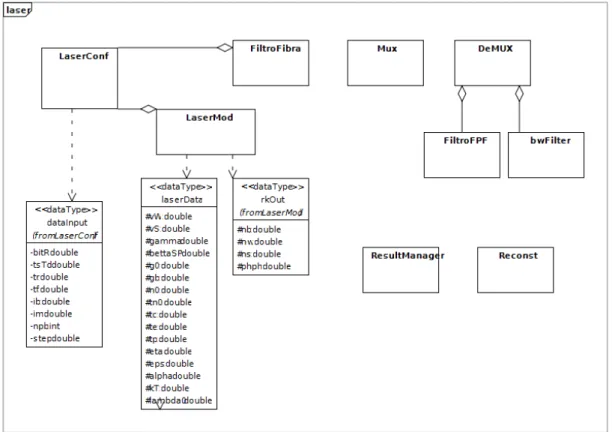
The developed User Interface (UI) is divided in several tabs, each one representing a part of the system allowing the user to configure each component and getting the feedback of the configuration defined. Each tab represents a class that contains the data and pointers to other objects that it depends on. The connections of each class is represented on the class diagram shown in figure 3.1. This dependencies have a logical sequence, once the user needs to configure the components through a certain sequence according to the pretended objective and to the sequence of events that happen in real systems. A namespace with utility methods was also implemented, providing the user several functions, avoiding the implementation of similar methods in each class. The objects implemented and the utility methods will be described and explained in the next sections.

Figure 3.1: Simplified Class Diagram of the simulator.

The UI was developed according to the problem, creating a user interface for data configuration, and three more, one to show the results in a graphical mode, showing

(34)

16

the generated charts, another, similar to the Windows c

Forms 1

MessageBox, once the needs for feedback messages were not fulfilled with the standard MessageBox and another Form that gives a feedback of the progress of the simulation when a file sending is simulated, with a progress bar and a message with the status of the progress. The steps (tabs) are developed in the next pages.

3.2.1 Laser Driver

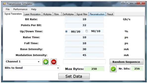
Figure 3.2: Laser Driver Tab of User interface.

The Laser Driver tab allows the user to configure some properties of the signal. On this configuration menu, the user have to provide the bit rate, the number of points per bit of the signal, the up/down time, the signal raise and fall time, the base intensity and the modulation intensity. On this menu, the user also defines the number of bits to transmit for each channel. The bit rate is the number of bits that are transmitted per second. This influences the time needed for data transmission, that can be computed with the formula:

Tsend= 1 BitRate∗ Nbits (3.1) 1 Windows c

(35)

The number of points per bit, is the number of points used to numerically represent, within the bit time, the signal associated with a given bit. The higher this value is,the more detailed is the output signal. This value is restricted to values that can be represented as 2

n

. Considering performance issues, this value is recommended to be less then or equal to 128 once values greater than this generate arrays to long, compromising the performance of the simulator. These two parameters, bit rate and number points per bit, are parameters that are not exclusive of the Laser Driver, once this values are parameters of the system and common to other elements of the simulator. The fall and raise times of the electrical signal are the time (in percentage) of the signal transition from 1 to 0 or from 0 to 1, respectively. The user has two options, being possible the choice of the raise of the signal between 20 and 80% or between 10 and 90% of the value of the signal corresponding to a bit 1 in steady state (assuming positive logic). This option will shape the signal according to the formulas on the appendix A.3. The predefined values were set as 10 ps. This value is acceptable once it was tested on article [20], where the values were tested for a 60 Gigabit per second (Gbps) bit rate. This field has no restriction.

The Base Intensity and Modular Intensity are the values of the current injected. The base intensity is the lower intensity, and the modular is the intensity of the step, leading to a maximum current intensity injected on the laser of Imax =Ibase+Imod. The input values have several options and might have several channels. When adding channels, a verification of the maximum number of channels is made according to the formula 3.3. For each channel a different kind of input can be selected. The user can use the pseudo-random bit generator, that generates a sequence of bits with the size selected on the number of bits field. The user can also select a file with the bit sequence to send, or select a file to send. The field Max Bytes limits the size of the input. In case a file has more elements than the Max Bytes field, the message represented in figure 3.3 is presented, allowing the user to cancel, to send only a part of the file with the size of Max Bytes, or to send the all parts of the file. This last option gives the user the possibility of define all parameters of all the steps, and the simulator separates the file or files to send in several pieces, according to the Max

(36)

18

Figure 3.3: _{Error provided when file exceeds Max Bytes value.}

The Signal Parameters Tab is the most restrained part, concerning to the data limits and restrictions. The restrictions on this option are at:

• Bit Rate

• _{Base Intensity and Modulation Intensity} • _{Max Bytes}

• _{Number of bits} • _{Number of Channels}

The bit rate parameter has a maximum value of 100 Gbps. This restriction was set based on the studies developed by [21], that was used as a reference during the simulator. The tested parameters were validated on that thesis, deciding not to allow higher values than 100 Gbps before deep tests. The Base and Modulation Intensity value has a restriction to avoid possible errors: Ib > 0and Im > 0.

The value of Max Bytes is restricted according to M ax Byt es ⇐ 1500 Bytes. This restrictions make sense on performance matters, limiting the resources needed to allocate all data and the time to execute the simulations, and on logical matters, once this value was defined taking in concern the Transmission Control Protocol (TCP) packet maximum size, once the algorithm of Multiple Description Coding (MDC) use a packet base transmission method.

The Number of Bits is restricted to a value of 12000 bits (1500 Bytes) with the same reasons of the Max Bytes restriction. The value is 1500 bytes according to TCP maximum payload.

(37)

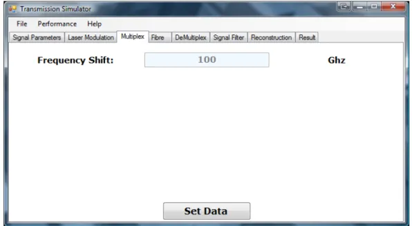
The Number of channels is validated according to the equation 3.3. The dividend returns the maximum frequency of the signal. To get the maximum number of channels that can be fitted on the signal, the maximum frequency is divided by the frequency deviation of each channel. According to the Telecommunication Standardization Sector (ITU-T) standard [38], the value of Dense Wavelength Division Multiplexing (DWDM) shift between each channel is 100 Ghz, simplifying the formula in 3.2, resulting in the formula presented in 3.3. Nchannels= BitRate ∗ Nppb ∆λ (3.2) Nchannels= BitRate ∗ Nppb 100∗ 10(9) (3.3)

3.2.2 Laser

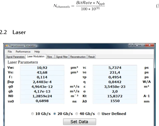
Figure 3.4: _{Laser Tab of User interface.}

The Laser tab allow the user to input the values of the laser configuration, allowing the user to insert the model of the laser needed for the experiment. The configurable parameters are represented at appendix A in section A.2 and showed in figure 3.4. The user can choose a laser configuration based on parameters estimated on [20] and on chapter 3 of [21]. There are three previously defined different configurations according

(38)

20

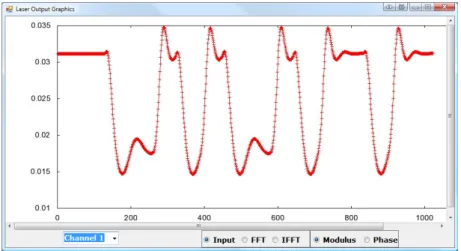
to the maximum speed the laser can support. The laser parameters can be input by the user or a model parameters can be selected. The configured models that can be selected are the models estimated in [21] to a maximum bit rate of 10 Gbps, 20 Gbps or 40 Gbps, with a comparative graph in [21] that shows the similarity of the parameters with real fibre. The user can also define a model based on the parameters of the values already defined clicking on the ’User Defined’ Radio Button, allowing the modification of the model values. The ’Set Data’ button induce the execution of the simulation code of the laser, explained with more detail at section 3.4.2. As a result, if the option is selected, the result of the operation is shown in a plot, using the ImageDisplay class, giving the user three plots, one with the result of the equation presented in the appendix A in section A.17 (modulus and phase in separated plots), the result of the Fast Fourier Transform (FFT) (the real part and the imaginary in separate), and the result of the Inverse Fast Furrier Transform (IFFT), having this last one a purpose of user analyses, once it have no use on the simulation.

Figure 3.5: Laser Result Window (input:1100101001011011).

An example of the result presentation of this module is represented in figure 3.5.

3.2.3 Multiplexer

The multiplexer tab, as figure 3.6 shows, has only one field. On this version of the simulator the modification of this value is not possible as a result of the value specified is a ITU-T standard [38]. The execution of the multiplexer is made without the perception of the user of the data manipulation, returning as a feedback to the

(39)

user, if the option selected, plots of the result of the operation, similar to figure 3.20. The implementation details of this feature are developed on section 3.4.5.

Figure 3.6: _{Multiplexer Tab of User interface.}

3.2.4 Fibre

(40)

22

The Fibre tab is where the user input the parameters to the fibre modelling, according to the formulas in the appendix A in section A.3. The UI of this module is represented in figure 3.7. On this module,the user has to set the fibre length (in Km), the first (1

st

) Order Dispersion. The dispersion is explained in more detail at section 3.4.4. The attenuation is another physic phenomenon that represents the reduction of the transmitted energy over the light carrying medium. This phenomenon is developed in section 3.4.4.

3.2.5 Demultiplexer

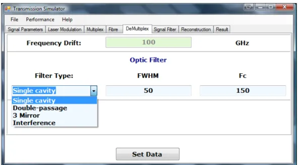
Figure 3.8: _{Demultiplexer Tab of User Interface.}

The Demultiplexer tab, as represented in figure 3.8, requires more parameters than the multiplexer, as a result of the elimination of part of the interference caused by the transmission of the signal and the filter requirements resulting in a more reliable and usable signal. The structure of this component is described in section 3.4.5. In result of the requirements to demultiplex the signal the user has to input the parameters of an optic filter. The optic filter can be chosen between a single cavity, double-passage, three (3) mirror and interference. For each one the value of Full Width at Half Maximum (FWHM), that is a parameter frequently used to characterize the with on a curve, that gives the distance between the points of the curve at which the curve reaches half of it’s maximum value. The Fc parameter is the filter fineness that is

(41)

used to compute the Free Spectral Range (FSR) described in the formula A.21 given in appendix A. The formulas and the implementation details are described in section 3.4.5. The restriction of this tab are the range of values of each box. The Frequency

Drift _{field is just an information field, once it was previously defined at the multiplexer}

tab, assuming the same value. The other fields have restrictions on the value, allowing only v alues > 0 and with 4 decimals.

3.2.6 Electrical Filter

Figure 3.9: _{Electrical filter tab.}

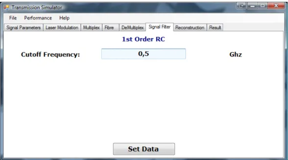
The electrical filter tab filters the signal resulting from the Demultiplexer tab or from the Fibre tab, if only one channel is defined. The operation done on this step is the application of an electronic filter, and Resistor-Capacitor (RC) filter. The purpose of the filter is to remove the interference caused by the multiplexing of the signal, and aliasing the signal removing the very high frequencies noise, smoothing the signal. The parameter necessary to the execution of the filter is the cut-off frequency of the filter. The default value of the filled is the value inserted in the Bit Rate inserted on

the Signal Parameters tab, being possible changed by the user to allow a more narrow or wide filtering, according to the user requirements. The implementation details of this step, as well as an explanation of the RC filter is developed in section

(42)

24

3.2.7 Signal Reconstruction

Figure 3.10: Reconstruction Tab of User Interface with all options enabled.

Figure 3.11: _{Example of an Eye Diagram.}

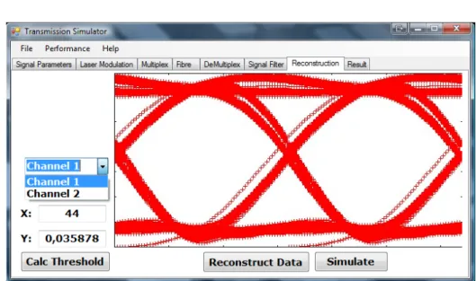
The reconstruction tab, as showed in figure 3.10, allows the user to reconstruct the signal, setting the values of the threshold. During this step the signal from the Demultiplexer (or the Fibre, depending on the number of channels)is analysed, and using the trheshol computed based on the eye diagram reconstructs the signal. The reconstruction of the signal is done considering the value defined by the user or computed and generates the signal, as explained in section 3.4.7. This tab can be shown to the user in two different ways, according to the type of simulation in execution. In case of the scenario is an array of bits transmission, or a file that have no need to

(43)

be splitted, the GUI presented is similar to the one presented in figure 3.10, without the button Simulate. If the input is a split file, only the Simulate button is showed, disabling all the other options, the channel selection and the x and y field. If the file to send is not split or a bit array is sent, the user have to define the threshold on this step clicking on the eye diagram or with the button Calc Threshold, that computes the value using the method described in section 3.4.7, to all channels defined or an error is shown. If the simulation is continuous, i.e., the transmission of several file parts, this step is computed with the same method, avoiding the user to intervene in the simulation.

The Eye Diagram is a useful way to analyse the quality of a signal, providing informations of the system performance, giving also information of the signal-to-noise, clock timing, Inter-Symbol Interference (ISI) among other information. The diagram is a oscilloscope display of the digital signal, with the repeated representation of the signal, as represented in figure 3.11. The eye diagram, in a purely digital system, gives the necessary information to test the integrity of the transmission system. The information that is possible to extract from this tool is very useful, since the ones described above, as long as information in order to compute the optimal sampling value to reconstruct the signal. More details of this subject can be found in [39] and [40].

3.2.8 Result

(44)

26

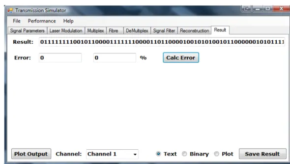
The Result tab presents the result of the simulation to the user. This step is only available in the case of a simulation of a bit array or a file part since the results of a continuous simulation is saved in a file as well as a file with the error information of each part. This part of the GUI, as represented in figure 3.12, gives the user to analyse the result of the simulation, as long as the possibility of the number of errors of the transmission, in absolute value and in percentage (%). The file containing the information of the simulation have the information:

- Number of bits transmitted

- Number of bit errors

- Number of burst errors

- Errors in percentage (%) of the resultant signal (comparing with the input)

The simulator also allows the user to save the result in a file, text or binary, or simply plot the data in a window or save the plot.

3.3 Object Oriented Architecture of the Simulator

The object-oriented programming (OOP) paradigm is widely used nowadays. This paradigm had a great disclosure, once it provides an approximation, when comparing to the procedural programming, to the real world, once in the real world the system is composed by objects. This paradigm also provides the developers an easier and faster way of code re-use, since each class models a part of the problem and is encapsulated, becoming easy the reuse of the code, and the expansion of the same, once it is not in the middle of a program. Besides those advantages, the code resulted is more structured once the functions of each object are well defined. This paradigm also has it downsides, the code generated using OOP is not so fast than the result of a procedural based program.

(45)

3.3. Object Oriented Architecture of the Simulator 27

Figure 3.13: Scheme of the developed Simulator classes.

When comparing the downsides and upsides, OOP is a good solution for develop-ment once the hardware used today are more than enough for the general applications developed, and the development time required is less, justified by the code reusing and the available library’s with developed classes. In a OOP paradigm, the objects are created by classes trading messages between them to get, set or trade some information or results.

For OOP projects modelling is very important, once, usually the projects developed with OOP are complex projects, with several classes, each one with even more attributes and methods, creating a complex development task and leading to results that cannot be the expected and/or the coordination and the messages traded between the objects malformed. To simplify this task, the Unified Modelling Language (UML) surges. The UML, as a language to model the application to develop, presents a standard

(46)

28

to characterize an application. Modelling the pretended solution, it avoids coding errors, and simplifies the task pf the development of the solution by a large team, once the specifications are defined. Concerning to the UML, there are several types of diagrams like the Class, Package, Use Case, Sequence among others, being those the most commonly used. The class diagrams describes the static structure of a system. With this diagrams the structure of the application is defined, representing the several classes, the connection/dependencies between them, and the data structures defined to solve the problem.

Figure 3.14: Scheme of the developed Simulator classes (continuation).

In figure 3.1 a simplified representation of the class diagram is showed. On this representation the data structures are defined, and the relation of each structure with the classes. The Utils namespace and the methods implemented on it are also represented in figures 3.13 - 3.14. This subject is developed with more detail in [41].

(47)

3.3. Object Oriented Architecture of the Simulator 29

Figure 3.15: _{Flowchart of the implemented simulator.}

The structure was designed as represented in figure 3.13 - 3.14 and defined after analysing the problem proposed to be solved. Once in real-world optic transmission has a structure/components as the represented in figure 3.16, the architecture of the simulator was defined as represented in figures 3.13 - 3.14. The system implemented consists in nine classes, three data structures, and a namespace of utility functions. The GUI was implemented using Visual Studio

c

2008 and Matlab. Visual Studio c

uses a wusiwug W hat U S eeI sW hat U G et method, generating the code of the UI. The classes and objects are instantiated in the main file, controlling the messages between the object and validating results. The Matlab software was used in the signal filtering, as explained at section 3.4.6.

(48)

30

3.4 Implementation Details

The simulator was developed using the object-oriented (OO) paradigm. Several mod-ules were developed, each one representing a component of the optical communication system. A simplified class diagram of the modules developed is shown in figure 3.13 and in figure 3.14. A simplified diagram is shown in figure 3.1.

Each module is described in this chapter, justifying the choices made for each one. The Multiple Quantum Well (MQW) laser may be modelled by a set of differential equations, equations A.4-A.7, which are provided in [21]. This model was chosen once it represents a close representation of reality, as represented in chapter 3 of [21].

The implementation of the interface was done using the Windows c

Forms, and the objects were implemented using C + +. The usage of C + + was a requirement of the project, once this language brings advantage on the high runtime efficiency as verified in [42]. The choice of Windows

c

Forms was made in consideration of the used language for codification (C++) and the integration of the language with the UI, providing an easy integration of both. The UI was developed using Microsoft

c Visual Studio c 2008, once this is a powerful tool do develop applications on the used language. During the development other choices where made with the purpose of improve the user experience and the application reliability. The implementation of the formulas and filters was a complex task due to the application and system requirements. This implementations are explained during this section.

3.4.1 Laser Driver

The laser driver is a component where the current intensity is modulated to send to the laser. The ideal scenario would be the one represented in figure 3.17(a), but in real world, the signal (in time domain) has a certain time to change state, as represented in figure 3.17(b).

(49)

3.4. Implementation Details 31

(a) Laser driver input (binary)

(b) Laser driver output

Figure 3.17: _{Input and Output data examples of the laser driver (input:1100101001011011).}

The signal parameters tab of the UI led to the implementation of utility methods, like the pseudo-random bit generator. This method was implemented applying the

rand() method of the st dlib library. This method is used to generate bit sequences to be sent by one channel when the option ’Bits to Send’ is selected. A feature of this component is the control of the size of the input signals, whether sequences or file parts. The size is controlled according to the first channel defined and/or by the

Max Bytes _value. _{In case the first channel is larger than the maximum value defined,}

a truncation or a continuous simulation is mandatory. When defining others channels, the size is controlled by the size of the first channel. If the channel to define is larger than the first one, the user can truncate the input of the channel or to extend the other channels already defined with a pseudo-random sequence that is ignored in the reconstruction feature. This feature is described in figure 3.18.

(50)

32

Figure 3.18: _{Input size control Flowchart.}

The user also have the option of select a certain part of the file, considering the max number of bits and the part the user wants to select. This is done using a auxiliary method that opens the file, shift the number of bytes necessary to start reading the data on the pretended position. When a file is transmitted, the reading is done byte-by-byte, decomposing each one in bits, shifting the byte-by-byte, getting the bit pretended. The solution used to set each channel was to set and validate each one step by step while it is defined, once this prevents the agglomeration of errors, becoming more user friendly the task of creating an error free configuration. The input is validated according to the size using: Nelements = 2

n_{, n ∈ N}

, once FFT has a better performance with arrays that meet this requirement. In the continuous simulation, the max Size is a unrestricted value, leading to a array with a size that does not fulfil the 2

n

requirement most of the times. The solution to this issue was to fill in the array until the size fulfil the requirements. The fill is done adding half of the bits at the beginning and the rest at the end. The number of elements added is kept in order to cut them out in the signal reconstruction.

(51)

When the button ’Set Data’ is pressed, the procedure that simulates the laser command circuit starts with fields validation, according to the restrictions explained at section 3.2.1, and set the objects with the parameters defined, generating, if the option is selected, the plots using files with the data to plot. The tool used to create the plots is Gnuplot [43]. The simulation of the command circuit is done based on the formulas A.1 - A.3 developed on appendix A.

3.4.2 Laser

The laser modelling models the behaviour of the MQW. The equations of the model described between section A.4 and A.7, were develop by Nagarajan et al. on [44] and by Ribeiro et al.. The formulas are used to get the derivative, applying the fourth (4

th ) order Runge-Kutta method, obtaining the results as a complex number in polar form, as a result of function described on section A.17. In detail, when the user click the ’Set Data’ the set and validation of parameters is performed, i.e. the conversion of the Strings inserted into numbers, returning am error message in case of error. The

LaserMod _{object instanced is set with the inserted values, or with a model selected}

with the values of table 3.1. When the parameters are defined and the object fields set, the laser modelling starts, applying the formula, applying the fourth (4

th

) order Runge-Kutta. This method was implemented using a base of the Numerical Recipes [45] method. Once the modelling is complete and the array of the pP(t) (modulus), and φ(t ) (phase), the FFT is performed, performing a transition from time domain to the frequency domain. To note that the FFT implemented performs the transform using arithmetic coordinates, forcing to convert the coordinates, using the formulas 3.4-3.5. The parameters of the models provided to 10, 20 and 40 Gbps are presented in table 3.1. The models used were proposed by [21].

P(t) = |Z | =px2₊_y2_,

(3.4)

φ = arg(Z ) = ±arctany

x, (3.5)

where Z is the Cartesian representation ( Z = x + iy ).

The result of the laser modelling is two arrays, one with the result of the equations described in section A.17, labelled as input once is the input of the FFT, and a second array with the result of the FFT as represented in figure 3.19(a) and 3.19(b).

(52)

34

(a) Plot of the Output power of the laser (b) Plot of the spectra at the output of the laser

Figure 3.19: _{Plots of Laser modelling (input:1100101001011011).}

10 Gb/s 20 Gb/s 40 Gb/s

Vw (Quantum Well Volume) ₁₈ 10.92 _23.425 µm

3

Vs (SCH Volume) ₇₂ _43.68 _93.7 µm

3 Γ(Optical Confinement Factor) _0.093 _0.114 _0.18715

βsp (Spontaneous Emission Factor) 10

−4 ₂_{.4403 ∗ 10}−4 ₉_{.8067 ∗ 10}−4

g0 (Linear Coefficient of Optical Gain) 4∗ 10

−12 ₄_{.9643 ∗ 10}−12 ₉_{.22 ∗ 10}−12 _m3_/s

gb (SCH Coefficient) 4.17 ∗ 10

−13 ₄_{.17 ∗ 10}−13 ₄_{.17 ∗ 10}−13 _m3_/s

N0 (Transparency Density) 1∗ −10

24 ₁_{.2859 ∗ 10}24 ₁_{.12348 ∗ 10}24 _{m − 3}

τn0 (Bimolecular Recombination Lifetime) 0.718 0.6898 _0.569935 ns

τc (Transport Time through SCH) 56.8 _5.7374 _7.4334 ps

τe (Thermionic Emission Time) 225 _231.4 _48.238779 ps

τp (Photon LifeTime) 3.95 _0.4954 _0.925391 ps

η (Face Quantic Differential Efficiency) 0.0442 _0.0442 _0.11 W /A

ε(Gain Compression Factor) 2.33 ∗ 10

−23 ₃_{.5450 ∗ 10}−23 ₁_{.808 ∗ 10}−23 _m3

α (Spectral Dilatation Factor) 3.22 ₂ ₂

Kt (Thermal Constant) 15.9 _15.8372 _10.468154 A

−1

λ0 (Emission Wavelength) 1532 ₁₅₅₀ ₁₅₇₅ nm

(53)

3.4.3 Multiplexer

(a) Channel 1 (b) Channel 2 (c) Channel 3 (d) Multiplexed signal

Figure 3.20: Spectra at the output of the Multiplexer with three (3) channels.

The multiplexer is a component that merges several inputs/channels into a single fibre, using different wavelengths. This operation brings a bandwidth expansion, for example, if 8 channels at 10 Gbps are merged in the wavelength dimension, a final net bandwidth of 80 Gbps is obtained. The optical multiplexer simulation is done according to the scheme showed in figure 3.20. The formula 3.6 describes the implementation of this module: σ = ( (n/2) ∗ Np, n = 2k k ∈ N −((n + 1)/2) ∗ Np, n = 2k + 1 k ∈ N (3.6)

(54)

36

where σ represents the number of elements to shift the signal, Np represents the number of elements to shift on the array. The number of elements is calculated using

Np = fmax_N_e , where Ne is the number of elements of the array and fmax is the maximum frequency of the signal, that is obtained using fmax =

FS

2 , where FS represents the sample frequency. This formulas are explained at [46].

3.4.4 Fibre

The fibre is the component that, in real world, is the mean used to transmit the optical signal with low losses. The fibre affects the signal with physical phenomenon, as an example of the attenuation and dispersion. There are other some phenomenon that can be ignore, once the effects of them are not significant, and ignoring them make possible the modelling of the Single-Mode Fibre (SMF). The validation of a model ignoring this phenomenon is develop by [21] on chapter 3.4. Considering this, the model implemented ignores the non-linear effects and the birefringence, as explained in [21]. This phenomenons are develop at [11], [47], [48], among others. The type of fibre considered on this model was a SMF, in consequence of the complexity of the multi-mode fibres phenomenons and consequent model complexity.

(a) Optical Loss according to window wavelength

(b) Attenuation propagation along the fibre

Figure 3.21: Fibre attenuation loss.

The attenuation is the reduction in the transmitted power [48]. This was the major problem on the optical communications during several years, once the first fibres produced presented a very high attenuation, around 1000 dB/Km, making the

(55)

transmission impossible. Nowadays, there are considerate three main wavelengths that are used with low optical levels that are represented in figure 3.21(a). The attenuation happens because of the absorption of the light signal through the fibre (and connections), and is caused by the impurity of the fibres and/or by the possible imperfections of the fibre. This phenomenon is represented in figure 3.21(b).

The attenuation is modelled in application according to the formula described in section A.19, getting as parameters the values configured at the UI.

On optics, the dispersion is the spreading of the pulse along the fibre. The bases of this phenomenon are explained at [47], but the importance for this dissertation is the consequences of it on optical transmission. The dispersion is caused because of the different speeds that different wavelengths propagates, causing the pulse to spread in consequence of that. The influence of this is schemed in figure 3.22, where is visible the initial pulses losing the intensity and spreading in time.

The dispersion can be inter-modal (or modal), or intra-modal. The first one occur only in multi-mode fibres, considering only the second one on our case, once this type (intra-modal) affects mono-mode and multi-mode fibres. The intra-modal dispersion can have two causes:

• _{Light propagates differently in the core and in the cladding of the fibre;} • _{Different wavelengths travel in wave-guide structures at different speed.}

Figure 3.22: _{Fibre dispersion phenomenon.}

The dispersion is a parameter defined by the user, and computed by the formula described in section A.18 along with the fibre transfer function. This parameter unit is in ps/(K m.nm).

The fibre module also allows the addition of noise to the signal. the noise spectral density is modelled as a noise parameter defined by the user, restricted in a range

(56)

38

between 0 and 1. This value is added to the phase component of the signal, causing the white noise on the channel.

3.4.5 Demultiplexer

The multiplexer allows the separation of the channels multiplexed with 3.4.3. The function of this component is to invert the multiplexer function with filters to select the channel and to reduce the interferences between the neighbour channels. This action is done using an optic filter. The optic filters implemented are Fabry-Perot filters, the single cavity, double-passage, three mirror and interference [21]. An example of each optical filter can be analysed in figure 3.23, where a plot of the transfer functions is represented.

Figure 3.23: _{Fabri Perot Filter transfer functions.}

The Fabri-Perot filter of single cavity was modelled by the formulas described in appendix A, with the formulas described in sections A.20-A.22. The value of the filter fineness considered as default was 150, once this is a value considered suitable in [21]. The double-passage Fabri-Perot filter, as suggested, uses a double passage of a single cavity filter, considering the same filter, i.e., considering the double-passage filter with two equal cavities. Considering this, the value of F W H M has the following

An object-oriented architecture for transmission simulation of image and video with multiple description coding over high-speed optical fibre channels