Dynamics in Hotelling based Models

(1)

Dynamics in Hotelling based Models

Department of Mathematics

Faculty of Sciences of University of Porto

June / 2015

(2)

Jorge Fernando Valentim Soares

Dynamics in Hotelling based Models

Thesis submitted to Faculty of Sciences of University of Porto, as a requisite to obtain the degree Master of Science in Mathematics,

under the supervision of Professor Alberto Adrego Pinto.

Department of Mathematics Faculty of Sciences of University of Porto

(3)

To my parents, for all.

To Professor Alberto Adrego Pinto, for the possibility to work with him, for his insights and support.

To all those who, one way or the other, helped me to become better.

(4)

Abstract

In 1929, Hotelling presented a model for spacial competition between two firms in which they compete in a two-stage game. First, both firms choose their location and after they choose their prices. In this work, we assume that the establishment of prices occurs in a dynamic way instead of a static one. We will use two different dynamics, namely, the Myopic Dynamics and the Best-Response Dynamics. Our main goal, will be to study the stability of the Nash Price Equilibrium. We also study the conditions that make the set of prices, for which every firm has a non-empty market share, a forward invariant set. For last, we will address the extension of the Hotelling model to a network, proposed by A. A. Pinto and T. Parreira. Again, we assume a dynamic establishment of prices and our goal is to study the stability of the Nash Price Equilibrium.

(5)

Em 1929, Hotelling apresentou um modelo de competição espacial entre duas firmas. Neste modelo, as firmas competem num jogo com duas etapas. Em primeiro lugar, as firmas escolhem a sua localização e, em seguida, escolhem o seu preço. Neste trabalho, nós iremos assumir que a escolha de preços ocorre de forma dinâmica. Iremos usar duas dinâmicas distintas, nomeada-mente, Myopic Dynamics e Best-Response Dynamics. O nosso objectivo, é estudar a estabilidade do equilíbrio de Nash em preços. Iremos também estudar as condições que tornam o conjunto de preços, para os quais as firmas partilham o mercado, num conjunto invariante. Por último, iremos estudar a extensão do modelo de Hotelling para uma network, proposto por A. A. Pinto e T. Parreira. De novo, iremos assumir a existência de uma escolha dinâmica de preços. O objectivo, é estudar a estabilidade do equilíbrio de Nash em preços.

(6)

List of Figures

3.1 Hotelling Model Diagram . . . 21

3.2 Duopoly Zone . . . 23

3.3 Shape of the Duopoly Zone in Case 2 . . . 24

3.4 Shape of the Duopoly Zone in Case 3 . . . 24

4.1 Shape of πAin Case A1 . . . 27

4.2 Shape of π_Ain Case A2 . . . 28

4.3 Shape of πAin Case B1 . . . 28

4.4 Shape of πAin Case B2 . . . 29

4.5 Partition of the Price Configurations Set . . . 32

5.1 Myopic Dynamics simulations. . . 45

5.2 Stability along Bh and Bv in Case 1 . . . 47

5.3 Stability along Bv in Case 2 . . . 48

5.4 Stability along Bh in Case 3 . . . 50

6.1 Example of Hotelling Network . . . 54

6.2 Indifferent Consumer in Hotelling Network . . . 55

(9)

Introduction

The model of spacial competition, introduced by Hotelling [6], has become an attractive framework to the study of oligopoly markets (see [5], [2], [13], [8] [1]). Hotelling, in his work, presented a city where the consumers buy a commodity from one of the two firms available. This city is represented by a segment line where the consumers are uniformly distributed. The firms, also located in the segment line, compete in a two-stage game. In first place, both firms choose their location and, afterwards, each one establishes the price for the commodity. In his first approach, Hotelling concluded that the firms would have an incentive to establish themselves in the center of the segment line. However, D`Aspremont et al. [5] showed that Hotelling`s conclusion is invalid. In this work, we will focus in the second stage of the Hotelling model by introducing a dynamical component. We consider that the firms continuously adjust the price of the commodity, instead of fixing the prices. Our goal is to study the stability of the Nash Price Equilibrium and the forward invariance of the Duopoly Zone. In addition, we intend to gain an insight in how the price of the commodity and market share of each firm varies with time. We will study the Hotelling model with different transportation and productions costs for both firms. We will utilize two different dynamics for the second sub game, namely, the Myopic Dynamics and the Best-Response Dynamics [9]. A. A. Pinto and T. Parreira [2], presented a model of an Hotelling town that generalizes the Hotelling model to a network, where the consumers and the firms are located. Like in the original Hotelling model, the consumers buy a single commodity from one of the firms available. In addition, the consumers are uniformly distributed along the edges of the network, also called roads. The firms compete, again, in a two stage game, choosing the location in the first sub game and the price

(10)

FCUP 10 Dynamics in Hotelling based Models

of the commodity in the second sub game. A. A. Pinto and T. Parreira introduced a condition, linking transportation costs, production costs and the topology of the network, that guarantees the existence of a Nash equilibrium in the price sub game.

In the last chapter of this work, we study the stability of the Nash Price Equilibrium in the Hotelling Network, assuming, that every firm adjusts is price accordingly to the principles of the Myopic Dynamics.

(11)

Basics of Game Theory and Dynamics

In this chapter, we will introduce some concepts of Game Theory and Differential Equations, that will be necessary in the rest of the text. Since the results are well known, some of them are presented without proof, but, in such cases, a reference is provided.

We will start by doing a brief introduction to differential equations and qualitative analyses.

2.1 Qualitative Analyses of Differential Equations

A system of differential equations inRnis given by a group of linked differential equations                      dx1 dt = f1(t, x1, . . . , xn) dx2 dt = f2(t, x1, . . . , xn) . . . dxn dt = fn(t, x1, . . . , xn) (2.1)

where each of the functions fi is defined in a open subset U ofRn, fi is real valued and at least

C0. The system 2.1 can be written in the abbreviated form

X` = F (t, X)

where X = (x1, . . . , xn)and F (t, X) = (f1(t, X), . . . , fn(t, X)), commonly referred to as a vector

field. If the system does not depend explicitly of the variable t, then we refer to it as an

(12)

tonomous system. We say that X(t; X_I) is a solution for system 2.1, with initial condition X_I, if

X`(t) = F (t, X) and

X(0; XI) = XI .

It is not guarantee, from the start, that such a solution exists or even if it is unique. An answer for this problem is given by the Theorem of Existence and Uniqueness of Solution (see [10]).

2.1.1 Stability

Definition 1. A point X0 ∈ Rnis an equilibrium point for a system of differential equations if F (t, X0) = 0 .

Now, we introduce a key notion in qualitative theory, that is the stability of an equilibrium point.

Definition 2. Let X0 ∈ Rnbe an equilibrium point for a system of differential equations:

• X0 is stable if

– for all ε > 0 there exists δ > 0 such that, if XI ∈ B(X0; δ)then X(t; XI)∈ B(X0; ε)for all t∈ R+.

• otherwise, X0is unstable.

• X0 is asymptotically stable if X0 his stable and

– there exists δ∗ > 0such that, if XI ∈ B(X0; δ∗)then X(t; Xi)→ X0as t→ +∞.

Informally, an equilibrium point X0 is stable, if a solution for the system that starts close of X0, remains close to X0, for all positive t. The point X0is asymptotically stable if it is stable and if there exists a neighborhood of X0, where the solution of the system converges to X0. A general method for investigating the stability of a fixed point was introduced by Lyapunov.

(13)

Definition 3. Let X₀ be an equilibrium point for a system of differential equations X` _{= F (t, X)} where F : U ⊆ Rn+1 _{→ R}n_{. A function V : D} _{⊆ R}n+1 _{→ R is a Lyapunov function for the above}

system if:

• D is a open subset ofRn+1_{and X}

0∈ D ⊆ U.

• V (X0) = 0and V (X) > 0 for all X ∈ D − {X0}.

• (V (X))` ≤ 0 for all X ∈ D − {X0}.

If the last condition is strict then V is a strict Lyapunov function .

Theorem 1. Let X0 be an equilibrium point for a system of differential equations, X` = F (t, X) where F : U ⊆ Rn+1_{→ R}n_.

• If there exists a Lyapunov function for the system then the equilibrium point is stable.

• If the Lyapunov function is strict then the equilibrium point is asymptotically stable.

A proof of this result can be seen in [10]. In the particular case where the system is autonomous, and all of the functions fi are affine, there exists a more direct way for proving the stability of an

equilibrium point.

Theorem 2. Let X`_{= F (X)}_{be a system of differential equations where F : U} _{⊆ R}n+1_{→ R}n_{is an}

affine vector field and X0 is an equilibrium point. Consider the matrix A that allows the system to be written as Y = AY + R and let{λi : 1 ≤ i ≤ n} be set of eigenvalues of A. If |λi| < 0, for all

1≤ i ≤ n, then X0 is asymptotically stable.

Another notion that will play a key role in this work, is the notion of a forward invariant set.

Definition 4. Let Γ be a subset ofRn_{and X(t; X}

I)a solution of a system of differential equations.

The set Γ is forward invariant if for all t≥ 0 and for all XI ∈ Γ

(14)

2.1.2 Lotka-Voterra Differential Equations

Now, we make an introduction a well-known class of differential equations called Lotka-Volterra. The most common example of a Lotka-Volterra type equation is the predator-prey equation pro-posed by Vito Volterra. This equation is given by

     dx dt = x(a− by) dy dt = y(−c + dx) . (2.2)

This equation models the dynamics of interacting populations of predators y and preys x . The parameters a and c represent the intrinsic growth of the respective species, while the parameters

band d represent the effect that one population has on the other population. We are interested in the generalization of this equation for an arbitrary number of species.

Definition 5. The general Lotka-Volterra type equation, for n populations, is of the form

dxi dt = xi(ri+ n ∑ j=1 aijxj) . (2.3)

The coefficients rirepresent the intrinsic growth of the population i and the parameter aij describe

the impact of the j-th population upon the i-th population. The matrix A = (aij)is often called the

interaction matrix.

This equation has a non-trivial equilibrium point, x∗= (x∗₁, . . . , x∗_n), determined by the linear system

n

∑

j=1

aijxj =−ri. (2.4)

If for all i ∈ {1, . . . , n} the components x∗_i satisfy x∗_i > 0 we call this equilibrium point feasible. Furthermore if A is non-singular then x∗exists and is unique.

Definition 6. Let A be a symmetric matrix of dimension n×n and real entries. A is called negative definite if all of its eigenvalues are negative. Equivalently, symmetric matrix A is negative definite

if

xTAx < 0

(15)

There are a number of results regarding the dynamic behavior of this type of differential equation (see for example [7]). In this work, we concentrate our attention in a result proved in 1977 by Goh [4] regarding the stability of a feasible fixed point of this type of differential equations.

Theorem 3. Assume that the general Lotka-Volterra equation has feasible fixed point x∗ = (x∗₁, . . . , x∗_n). In addition, assume that the interaction matrix A is non-singular. If there exists a constant positive diagonal matrix C, such that, CA + ATC is negative definite then x∗ is asymptotically stable with a Lyapunov function given by

V =

n

∑

n

ci[xi− x∗i − x∗iln(xi/x∗i)] .

Proof. Assume that exists a positive diagonal matrix C = (c1, . . . , cn), such that, CA + ATC is

negative definite. The function

V =

n

∑

i=1

ci[xi− x∗i − x∗iln(xi/x∗i)]

has a global minimum at (x∗₁, . . . , x∗_n).

Using 2.4, the derivative of this function computed along the solutions of equation 2.3 is given by

dV dt(X) = n ∑ i=1 ci(x1− x∗i)( dxi/dt xi ) = n ∑ i=1 ci(xi− x∗i)(ri+ n ∑ j=1 aijxj)by 2.4 = n ∑ i=1 ci(xi− x∗i) n ∑ i=1 aij(xj− x∗j) = 1 2(x− x ∗₎T_{(CA + A}T_C)(x_{− x}∗_{) .}

Since CA + AT_C _{is negative definite then} dV

dt(X)is negative, for all x ̸= x∗, and V is indeed a

Lyapunov function for 2.3 which concludes the proof.

This insights regarding Lotka-Volterra equations will be particularly useful in Chapter 4 and 6. The last result of this section, is a theorem proved by Gershgorin (see [15]) concerning the eigenvalues of an arbitrary matrix.

Theorem 4. Let A be a matrix with dimension n× n. Then all of its eigenvalues lie into, at least,

one of the discs

(16)

where R_i=∑n_j_̸=i|aij|.

In the next section, we introduce some useful concepts of Game Theory.

2.2 Basics in Game Theory

The field of Game Theory started from very sporadic considerations, made by authors like E. Zermelo [16], E. Borel [3] or Steinhaus [14], to a widely considered approach to economic theory. Most of this path was walked by John Von Neuwman and Oskar Morgenstern, a collaboration which ultimately led to the publication of the book entitled Theory of Games and Economic Behavior. Later on, John Nash gives his contribution to the theory of non cooperative games (see [11]). He was awarded with the Nobel Prize in Economics and since then many more have won this prize for their contributions in this area.

Informally a game can be described as a set of players, who are matched, to take some actions, chosen from a given set. An utility function is attached to every player, that determines his utility, given a combination of actions, taken by all the players. The objective of each player is to maximize his utility function.

Definition 7. A game is described by the quadruple

G =< I, M, (Si)i∈I, (πi)i∈I >

where:

1. I ={1, 2, . . . , n} is the set of types of players;

2. M ={m1, m2, . . . , mn} specifies the number of players for type i;

3. for every i∈ I, Si is the closed set of strategies (or actions) for each player type;

Defining mj(i) = mj if j ̸= i and mi(i) = mi− 1 the function

πi:×j∈IS mj(i)

(17)

πi(s−i; si) = πi((s11, . . . , sm11, . . . , s

mn

1 , . . . , s

mn

n ); si)

represents the utility obtained by the player i when he plays si and the other players play the

combination of strategies s_−i.

Keep in mind that a player objective, in any game, is to maximize his utility function, thus the next logical step is to know the strategy or strategies that maximizes the utility function, given the other players strategies.

Definition 8. Given a game G and a vector of strategies s_i,

BRi(s−i) = argmaxsi∈Sπi(s−i; si)

is the set of best response strategies for player i given the combination of actions s_−itaken by the other players.

Let BR(S) = (BR1(s−1), . . . , BRi(s−i), . . .). We note that the set BR() might not define a best

response function, because BR() might be only a correspondence between strategies. Now, we state one of the most important concepts in Game Theory, the Nash Equilibrium.

Definition 9. A strategy vector x∗∈ ×j∈IS mj(i)

j × Si is a Nash Equilibrium if

x∗ ∈ BR(x∗) .

Example 1. A classical example of a game is the so called Prisoner`s Dilema.

Suppose that two members of a criminal gang are caught by the police and that the prosecutors do not have enough evidences to convict the pair on the charges. In order to solve this problem they put the criminals in different rooms, and simultaneously they offer them the following deal:

• Betray the other criminal, by testifying that they have committed the crime. (B) • Stay silent. (S)

Formally, we define this game by having two players{α, β} of the same type with a discrete set of strategies, namely{B, S}. The payoffs are summarized in table 2.1.

(18)

α, β B S

B (1,1) (0,3)

S (0,3) (2,2)

Table 2.1: Utilities for the Prisoner`s Dilemma.

Each pair (i, j), of table 2.1, means that the players α,β will get i and j years in jail, respectively, when they play the corresponding strategies. The Best-Response correspondence is

BRα(B) = S

BRα(S) = S

BRβ(B) = S

BRβ(S) = S

Hence, it follows that the Nash Equilibrium is the pair of strategies (S, S) were each of the criminals gets two years in jail. Interestingly, if the players choose to play (B, B) each of them would only get one year in jail, which is better than what they gain by playing (S, S). This is a canonical example, were pure "rational" behaviors, in the sense that players only try to maximize their utilities, might not lead to the best choices.

Definition 10. Given a game G, we say that the players are choosing their strategies accordingly

to the Best-Response Dynamics if

dsi

dt ∈ BR(s−i)− si (2.6)

where BR(s_−i)denotes the Best-Response Correspondence of player i given the strategies of all the other players.

This Best-Response Dynamics was introduced by Matsui [9]. We note that equation 2.6 does not necessarily define a differential equation since BR() may only be a correspondence and not a function. A big number of results concerning the Best Response Dynamics have been proven for general games. A simple result linking the Best-Response Dynamics to the Nash Equilibrium is the following.

Definition 11. Given a game G =< I, M, (Si)i∈I, (πi)i∈I >then S∗ is a Nash Equilibrium if, and

(19)

In the case of the Hotelling model that we analyze in this thesis, the Best-Response Dynamics thus in fact define a differential equation. Our objective, is to use the tools exposed in the last section to investigate the stability of the Nash Equilibrium. We will also investigate the asymptotically properties of the solutions in order to obtain some economical insight. This field of Game Theory is normally referred to as Evolutionary Game Theory.

(20)

Chapter 3

Hotelling Model

In 1929, H. Hotelling [6] introduced a spacial model of a competition between two firms. In this model firms are located along a segment line of given length l and sell the same commodity at prices pAand pBrespectively. The consumers are uniformly distributed along the line and buy one

unity of product at each unit of time. The price P payed by the consumers is given by the price at which they buy the commodity, pAor pB, plus a transportation cost per unit of distance. We will

consider that this transportation cost can be different, tA or tB, depending of the firm where the

consumer buys the product. We consider that each firm has a unitary production cost cA and cB

corresponding to the price the firms pay per one unity of the commodity. From the point of view of game theory there are two sub games to be considered in this model, first the firms choose their location and afterwards the firms choose their prices. In this work, we will mainly concentrate on the price sub game assuming that the firms are located in the extremes of the line.

3.1 Indifferent Consumer and Profit

In a game the goal of the players is to maximize their utility, with this fact in mind is logic to consider that the firms will try to sell their product at the highest price possible. On the other hand, each consumer will buy at the firm that guaranties him the lowest price P . Now, we introduce the

indifferent consumer that is important to determine the profits of both firms. If both firms have a

non-empty market share the indifferent consumer x is the consumer who pays the same price 20

(21)

for the commodity whether he buys at firm A or firm B, that is

pA+ tAx = pB+ tB(l− x) . (3.1)

If the firm A supplies the whole market then the indifferent consumer is taken to be x = l. On other hand if the firm B supplies the whole market then the indifferent consumer is taken to be x = 0.

Figure 3.1: Hotelling Model Diagram

Lema 1. Given a price configuration (pA, pB)the indifferent consumer is given by

x(pA, pB) =              l if p_B− p_A≥ t_Al pB−pA+tBl tA+tB if − tBl < pB− pA< tAl 0 if pB− pA≤ −tBl . (3.2)

Proof. In the computation of x there are three cases to consider:

1. The firm A supplies the whole market;

2. Both firms have a non-empty market share, that is 0 < x < l; 3. The firm B supplies the whole market;

Suppose that firm A supplies the whole market then the price payed by the consumer located in the end of the line satisfies

pA+ tAl≤ pB.

If firm B supplies the whole market then the consumer located in the beginning of the line satisfies

(22)

If both firm are sharing the market then the indifferent consumer satisfies

pA+ tAx = pB+ tB(l− x) . (3.3)

Solving for x, we obtain

x = pB− pA+ tBl tA+ tB

. (3.4)

In this case x satisfies 0 < x < l and so

−tBl < pB− pA< tAl .

Since we are interested that both firms have a non empty market share, that is 0 < x < l, we introduce the following definition of the Duopoly Property.

Definition 12. A price configuration (pA, pB)satisfies the Duopoly Property if, and only if,

−tBl < pB− pA< tAl . (3.5)

We observe that pA ≥ cA and pB ≥ cB to guarantee have a non-negative profit. The definition

of indifferent consumer allows us to define the profit functions for the Hotelling game. Observe that the indifferent consumer x(pA, pB)represents the numbers of consumers that buy on firm A.

Therefore the profit of a firm A is given by its profit margin pA− cAtimes the number of consumers

x(pA, pB)that buy at firm A. Hence,

πA= πA(pA, pB) =              (pA− cA)l if pA≤ pB− tAl (pA−cA)(pB−pA+tBl) tA+tB if − tBl < pB− pA< tAl 0 if pA≥ pB+ tBl . (3.6)

The reasoning behind the profit of firm B is analogous, however, we need to have in consideration that the number of clients, in this case, is given by l− x(pA, pB). Hence,

πB= πB(pA, pB) =              (pB− cB)l if pB≤ pA− tBl (pB−cB)(pB−pA+tBl) tA+tB if − tBl < pB− pA< tAl 0 if p_B≥ p_A+ tAl . (3.7)

(23)

3.2 The Duopoly Zone

The Duopoly Property in conjunction with pA ≥ cA and pB ≥ cB, allows us to give a geometric

interpretation of the set of price configurations, for which, the firms are sharing the market. From now on, we refer to this set of prices as Duopoly Zone. Hence, figure 3.2 represents one of the

Figure 3.2: Duopoly Zone

possible shapes of the Duopoly Zone. The horizontal and vertical boundaries of the Duopoly Zone are given, respectively, by the sets

Bh ={(pA, cB) : pA≥ cAand (pA, cB)has Duopoly Property} (3.8)

Bv ={(cA, pB) : pB≥ cBand (cA, pB)has Duopoly Property} (3.9)

On other hand, the superior and inferior diagonal boundaries of the Duopoly Zone are represented, respectively by

Bs ={(pA, pB) : pB= pA+ tAland pA> cA} (3.10)

Bi ={(pA, pB) : pB= pA− tBland pB > cB} (3.11)

We note that above the boundary Bs, the firm A supplies the whole market and the indifferent

consumer is x = l. Below the boundary Bi, the firm B supplies the entire market and the indifferent

consumer is x = 0.

(24)

There are three possibilities for the shape of the Duopoly Zone depending upon the following inequalities:

1. −tBl < ∆c < tAl;

2. ∆c≤ −tBl;

3. ∆c≥ t_Al;

In the first case, point (cA, cB)has the Duopoly Property. Hence, the Duopoly Zone has the shape

represented by figure 3.2. In the second case, point (cA, cB)belongs to the boundary Bior is below

the boundary the Bi. Figure 3.3 represents the shape of the Duopoly Zone in case 2. The last

(a) Case ∆c =−tBl (b) Case ∆c <−tBl

Figure 3.3: Shape of the Duopoly Zone in Case 2

case is symmetric to case 2 and point (cA, cB) belongs to the boundary Bs or is above boundary

Bs. Figure 3.4 represents the shape of the Duopoly Zone in the last case.

(a) Case ∆c = tAl (b) Case ∆c > tAl

(25)

We observe that, in cases 2 and 3 one of the firms has an advantage in the competition. In case 2, the firm B can throw firm A out of the market without having to lower its price to values near its production cost. In case 3, the advantage belongs to firm A, who can throw firm B out of the market without having to lower its price near its production cost.

As a final note, we make a remark regarding the lines with slope one located inside the Duopoly Zone. Along these lines, the market share of each firm remains constant. If the firms start, at some point, to collaborate they can raise the prices by the same amount changing their market-shares. From the consumer point of view this is not good, because they can end paying a lot more for the product. So this discussion justifies the introduction of mechanisms to protect the consumer from this possible firm cooperation, specially in markets where the commodity being sold is essential.

(26)

Chapter 4

Best-Response Dynamics

In this chapter, our objective is to find the Best-Response Dynamics for the Hotelling Model. First of all, we need to focus our attention in finding the Best-Response Correspondence of each of the firms. Since the profit functions are similar for both firms, we concentrate in finding the Best-Response Correspondence for firm A.

4.1 Dynamics

We recall that the profit πAis given by

πA= πA(pA, pB) =              (pA− cA)l if pA≤ pB− tAl (pA−cA)(pB−pA+tBl) tA+tB if − tBl < pB− pA< tAl 0 if pA≥ pB+ tBl . (4.1)

The second branch of the profit function is a concave quadratic function in pA, with zeros given by

pA= cAand pA= pB+ tBl. Consequently, admits a maximum point for pA= pB+tB₂l+cA. However,

this point may not be the global optimum for πA. We are going to show that the form and maximum

of πAwill depend on the relative position in the line of the four possible maximum candidates,

cA, pB+ tBl,

pB+ tBl + cA

2 , pB− tAl . (4.2)

Let us suppose, that the smaller value is pB + tBl then, we obtain that pB + tBl ≤ pB − tAl.

This is an absurd, since the transportation costs are positive and not necessarily equally. On the 26

(27)

other hand, consider that the smaller value is pB+tBl+cA

2 then, we obtain that

pB+tBl+cA

2 ≤ cAand

pB+tBl+cA

2 ≤ pB + tBl. This is an absurd since

pB+tBl+cA

2 is the middle point between cA and pB+ tBl. Therefore, there are only two cases:

• Case A, where pB− tBlis the smallest maximum candidate in 4.2.

• Case B, where cAis the smallest maximum candidate in 4.2.

Consider Case A:

There are two hypothesis for the relative position of the maximum candidates in 4.2.

• Case A1 pB− tAl≤ cA≤ pB+ tBl + cA 2 ≤ pB+ tBl . (4.3) • Case A2 pB− tAl≤ pB+ tBl≤ pB+ tBl + cA 2 ≤ cA. (4.4)

In figure 4.1, we show, in Case A1, the graphic representation of πA. From the graphic

represen-Figure 4.1: Shape of πAin Case A1

.

tation of πAin Case A1, is possibly to verify that, given a price pB, the profit of firm A is maximum

when pA= pB+tB₂l+cA, that is

arg max πA(pA; pB) =

pB+ tBl + cA

2 . (4.5)

Consider Case A2:

(28)

be zero independently of the price set by firm A, so the maximum profit is achieved at p_A= cAand

arg max πA(pA; pB) = cA. (4.6)

Figure 4.2: Shape of πAin Case A2

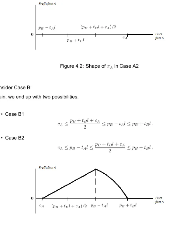
Consider Case B:

Again, we end up with two possibilities.

• Case B1 cA≤ pB+ tBl + cA 2 ≤ pB− tAl≤ pB+ tBl . (4.7) • Case B2 cA≤ pB− tAl≤ pB+ tBl + cA 2 ≤ pB+ tBl . (4.8)

Figure 4.3: Shape of πAin Case B1

Consider Case B1:

(29)

that, given p_B, the profit of firm A is maximum at p_A= pB− tA, that is

arg max πA(pA; pB) = pB− tAl . (4.9)

Consider Case B2:

Figure 4.4: Shape of πAin Case B2

The picture 4.4 shows, that if pB satisfies Case B2, then firm A achieves is maximum profit by

setting is price at pB+tBl+cA

2 and

arg max πA(pA; pB) =

pB+ tBl + cA

2 . (4.10)

The above discussion leaves us in position to compute the Best-Response Correspondence for firm A.

Theorem 5. The Best-Response Correspondence for firm A, BrA(pB), is:

BrA(pB) =              pB− tAl if pB ≥ cA+ tBl + 2tAl pB+cA+tBl 2 if cA− tBl < pB < cA+ tBl + 2tAl cA if pB ≤ cA− tBl .

Proof. Given a price pB, it was already shown that there are four different cases for the shape of

firm`s A profit function. The four cases can be joined, accordingly to the point where the global maximum is achieved. We end up with three groups:

• Case B1 - πAas a global maximum at pA= pB− tAl.

• Case B2 and Case A1 - πAas a global maximum at pA= (pB+ tBl + cA)/2.

(30)

Case B1 is characterized by

cA≤

pB+ tBl + cA

2 ≤ pB− tAl≤ pB+ tBl .

Since pB− tAl≤ pB+ tBland that (pB+ tBl + cA)/2is the middle point between cAand pB+ tBl,

we obtain that Case B1 is also defined by the system of inequalities given by      cA ≤ pB+ tBl pB ≥ cA+ tBl + 2tAl .

Since pB ≥ cA+ tBl + 2tAlimplies cA≤ pB+ tBlthen Case B1 is fully characterized only by the

first inequality. Therefore, if pB≥ cA+ tBl + 2tAlthen arg max πA(pA; pB) = pB− tAl . Case A2 is characterized by pB− tAl≤ pB+ tBl≤ pB+ tBl + cA 2 ≤ cA.

Again, considering that pB−tAl≤ pB+ tBland since, (pB+ tBl + cA)/2is the middle point between

cAand pB+ tBl, we obtain that Case A2 is also fully characterized by

pB+ tBl≤

pB+ tBl + cA

2 .

With some computations, we verify that Case A2 is characterized only by

pB≤ cA− tBl .

Therefore, if pB≤ cA− tBlthen

arg max πA(pA; pB) = cA.

Consider now Case B2 and Case A1 characterized by

cA≤ pB− tAl≤ pB+ tBl + cA 2 ≤ pB+ tBl or pB− tAl≤ cA≤ pB+ tBl + cA 2 ≤ pB+ tBl .

(31)

For the same reasons pointed in the previous cases, we verify that Case B2 and Case A1 are characterized by cA− tBl≤ pB ≤ cA+ tBl + 2tAl . Hence, arg max πA(pA; pB) = pB+ tBl + cA 2 .

By symmetry, we set the Best-Response Correspondence for firm B.

Theorem 6. The Best-Response Correspondence for firm B, BrB(pA), is given by

BrB(pA) =              pA− tBl se pA≥ cB+ 2tBl + tAl pA+cB+tAl 2 cB− tAl < pA< cB+ 2tBl + tAl cB se pA≤ cB− tAl .

Recall the definition of the Best-Response Dynamics given in chapter 1. As a corollary of the last two theorems we set the main result of this section.

Corollary 1. In the Hotelling model, the Best-Response Dynamics is given by

dpA dt =              pB− tAl− pA if pB ≥ cA+ tBl + 2tAl pB−2pA+cA+tBl 2 if cA− tBl < pB< cA+ tBl + 2tAl cA− pA if pB ≤ cA− tBl dpB dt =              pA− tBl− pB if pA≥ cB+ 2tBl + tAl pA−2pB+cB+tAl 2 if cB− tAl < pA< cB+ 2tBl + tAl cB− pB if pA≤ cB− tAl .

The Best-Response Dynamics separates the set of price configurations into nine different regions.

• Region A11given by [0, cB− tAl]× [0, cA− tBl].

• Region A12given by [cB− tAl, cB+ tAl + 2tBl]× [0, cA− tBl].

(32)

• Region A₂₁given by [0, c_B− t_Al]× [cA− tBl, cA+ 2tAl + tBl]. • Region A22given by [cB− tAl, cB+ tAl + 2tBl]× [cA− tBl, cA+ 2tAl + tBl]. • Region A23given by [cB+ tAl + 2tBl, +∞[×[cA− tBl, cA+ 2tAl + tBl]. • Region A31given by [0, cB− tAl]× [cA+ tBl + 2tAl, +∞[. • Region A32given by [cB− tAl, cB+ tAl + 2tBl]× [cA+ tBl + 2tAl, +∞[. • Region A33given by [cB+ tAl + 2tBl, +∞[×[cA+ tBl + 2tAl, +∞[.

Figure 4.5 shows the prices partition in these regions. Recall that the dynamical equilibrium points

Figure 4.5: Partition of the Price Configurations Set

of the Best-Response Dynamics are the Nash equilibrium points. We can find the Nash Price Equilibrium using the above prices partition.

Theorem 7. In the Hotelling model, there exists a Nash Price Equilibrium with Duopoly Property

if, and only if,

−2tBl− tAl < ∆c < 2tAl + tBl .

(33)

Proof. In Region A₁₁the equilibrium point is given by      cA− pA = 0 cB− pB = 0 .

Consequently, (cA, cB)is an equilibrium point for the system. However, this point is not necessarily

located inside Region A11. In fact, (cA, cB)is only located in this zone if, and only if,

cA≤ cB− tAland cB≤ cA− tBl,

which is absurd, hence there are no equilibrium points in this zone. Utilizing similar arguments, we conclude that in Regions A12,A13,A21,A23,A31,A32 and A33there are no equilibrium points for the Best-Response Dynamics.

Consider Region A22. The equilibrium points are given by      pB−2pA+cA+tBl 2 = 0 pA−2pB+cB+tAl 2 = 0 .

Therefore, the equilibrium point is

P∗= ( 2cA+ cB+ 2tBl + tAl 3 , 2cB+ cA+ 2tAl + tBl 3 ) .

This point falls inside Region A22if, and only if,

cB− tAl < 2cA+cB+2t₃ Bl+tAl < tAl + 2tBl + cB

cA− tBl < 2cB+cA+2t₃ Al+tBl < 2tAl + tBl + cA.

Hence, there exits a Nash Price Equilibrium if, and only if,

−2tBl− tAl < ∆c < 2tAl + tBl . (4.11)

We only need to verify, that under the above condition, this Nash Price Equilibrium has Duopoly property. In fact, the indifferent consumer at P∗satisfies

(34)

4.2 Stability of the Nash Price Equilibrium

In this section, we proceed under the assumption that the Nash Price Equilibrium exists. The first question we want to answer, regarding the price evolution under the Best-Response Dynamics is:

• Consider that the initial prices are sufficiently close to the Nash Price Equilibrium, which are the trajectories followed by the prices?

This question is mathematically corresponds to study of the stability of an equilibrium point, pre-sented in chapter 2.

Theorem 8. The only Nash Price Equilibrium point

P∗= ( 2cA+ cB+ 2tBl + tAl 3 , 2cB+ cA+ 2tAl + tBl 3 ) is asymptotically stable.

Proof. Inside Region A22the Best-Response Dynamics can be written as  dpdtA dpB dt   =  −1 12 1 2 −1    pA pB   +  cA+t2Bl cB+tBl 2  

Hence, the Best-Response Dynamics in Region A22is affine. The system matrix has two negative eigenvalues, λ1=−1₂ and λ2=−3₂. This implies that the Nash Price Equilibrium is asymptotically stable.

Theorem 8 does not imply that, for every initial condition inside the Duopoly Zone or even Region

A22, the price trajectory will converge into the equilibrium point. Since the Best-Response Dynam-ics is defined taking into account different zones of the plane, at this point, we can only guarantee that exists an open set of price configurations around the Nash Price Equilibrium, for which the price trajectory will converge to the equilibrium point.

4.3 Invariance of the Duopoly Zone

(35)

• Given a price a configuration in the Duopoly Zone, does any of the firms ends with an empty market share?

Mathematically, we address this question as follows:

• Is the Duopoly Zone a forward invariant set for the Best-Response Dynamics?

First we state a result about the invariance of the set of prices given by [cA, +∞[×[cB, +∞[.

Lema 2. The set of prices, defined by [cA, +∞[×[cB, +∞[, is a forward invariant set for the

Best-Response Dynamics.

Proof. The proof of this result follows directly from the fact that the Best-Response

Correspon-dence never drops bellow cAfor firm A and bellow cB for firm B. The direction of the vector field

along pA= cAis fully characterized by the sign of dpA/dt. This derivative is given by

dpA dt =              pB− tAl− cA if pB≥ cA+ tBl + 2tAl pB−cA+tBl 2 if cA− tBl < pB < cA+ tBl + 2tAl 0 if pB≤ cA− tBl .

Therefore, dpA/dt≥ 0 along the line pA = cA. This implies that a solution of the Best-Response

Dynamics never crosses the line pA= cA. A similar argument allows to prove that a solution of the

Best-Response Dynamics never crosses the line pB = cB. The combination of these two results

proves the claim of the lema.

Lema 2 has a very acceptable and expected economic interpretation. Given any initial price configuration, non of the firms has an advantage in dropping the price bellow their respective production cost.

We also observe, that theorem 2 implies that a solution of the Best-Response Dynamics, with initial condition inside the Duopoly Zone, never leaves this zone by the boundaries B_h and Bv.

The next result determines sufficient conditions for the invariance of the Duopoly Zone under the Best-Response Dynamics.

Theorem 9. If a Nash Price Equilibrium with Duopoly Property exists, then the Duopoly Zone is a

(36)

Proof. To prove this theorem, we only need to prove, that if a Nash Price Equilibrium with Duopoly

Property exists then the Best-Response Dynamics vector field points inwards, along the boundaries

Bs and Bi of the Duopoly Zone. Now, by Corollary 1 the components of the vector field along Bs

are given by dpA dt =              0 if pA≥ cA+ tBl + tAl −pA+cA+tBl+tAl 2 if cA− tBl− tAl < pA< cA+ tBl + tAl cA− pA if pA≤ cA− tBl− tAl and dpB dt =              −tBl− tAl if pA≥ cB+ 2tBl + tAl −pA+cB−tAl 2 if cB− tAl < pA< cB+ 2tBl + tAl cB− pA− tAl if pA≤ cB− tAl .

We will study, separately, three different cases:

1. −t_Bl < ∆c < tAl.

2. −2tBl− tAl < ∆c≤ −tBl.

3. tAl≤ ∆c < 2tAl + tBl.

Consider that−tBl < ∆c < tAl. The following relation of order is satisfied

cA− tBl− tAl≤ cB− tAl≤ cA≤ tBl + tAl + cA≤ tAl + 2tBl + cB .

The last inequality divides the line p_B= pA+ tAlin six segments, where different branches of the

Best-Response Dynamics are valid. The vector field along those segments is given by:

1. if pA∈] − ∞, cA− tBl− tAl]then      dpA dt = cA− pA dpB dt = cB− pA− tAl . 2. if p_A∈]c_A− t_Bl− tAl, cB− tAl]then      dpA dt = −p A+cA+tAl+tBl 2 dpB dt = cB− pA− tAl .

(37)

3. if p_A∈]c_B− t_Al, cA]then _     dpA dt = −p A+cA+tAl+tBl 2 dpB dt = −pA+cB−tAl 2 . 4. if pA∈]cA, cA+ tBl + tAl]then      dpA dt = −p A+cA+tAl+tBl 2 dpB dt = −p A+cB−tAl 2 . 5. if pA∈]cA+ tBl + tAl, tAl + 2tBl + cB]then      dpA dt = 0 dpB dt = −p A+cB−tAl 2 . 6. if pA∈]tAl + 2tBl + cB, +∞[ then      dpA dt = 0 dpB dt = −p A+cB−tAl 2 .

Considering that Bs is limited by pA = cA, we only need to consider the last three cases. If pA ∈

]tAl + 2tBl + cB, +∞[ or pA∈]cA+ tBl + tAl, tAl + 2tBl + cB], the first component of the vector field is

zero, therefore the vector field point inwards if, and only if, dpB/dt≤ 0. If pA∈]tAl + 2tBl + cB, +∞[

we obtain

dpB

dt =−(tA+ tB)l < 0 ,

and the vector field points inwards. If pA∈]cA+ tBl + tAl, tAl + 2tBl + cB]and since pA≥ cA, we

obtain dpB dt = −pA+ cB− tAl 2 ⇒ dpB dt ≤ ∆c− tAl 2 .

Therefore, under the condition−tBl < ∆c < tAl, we obtain that dpB/dt < 0and the vector field

points inwards.

Finally, consider that pA∈]cA, cA+ tBl + tAl]. Under the condition−tBl < ∆c < tAlwe obtain

dpB dt = −pA+ cB− tAl 2 ⇒ dpB dt ≤ ∆c− tAl 2 .

(38)

If p_Ais between c_Aand c_A+ tAl + tBlwe obtain

dpA dt = −pA+ cA+ tAl + tBl 2 ⇒ dpA dt ≥ 0 .

This implies that Best-Response Dynamics vector field points inwards along the boundary Bs.

A similar argument, allows to prove that the Best-Response Dynamics vector field, also points inwards in the case where−2tBl− tAl < ∆c ≤ −tBland tAl ≤ ∆c < 2tAl + tBl. By symmetry,

the Best-Response Dynamics vector field, also points towards the interior of the Duopoly Zone along the boundary B_i. Since, a solution of the Best-Response Dynamics never crosses the lines

pA= cAand pB = cB, the prove follows.

The fact that the Duopoly Zone is a forward invariant set for the Best-Response Dynamics brings very interesting consequences from the economic point view. First of all, if a Nash Price Equilibrium with Duopoly Property exists, non of the firms has an incentive to supply the whole market. This behavior makes the market very resistant to fluctuations resulting from outside factors. Facing an unexpected fluctuation in the market share a firm never drops out the market as long it keeps a tiny number of customers.

In the last discussion, we were assuming that the difference between production costs allows the existence of a Nash Price Equilibrium with Duopoly Property. It is also interesting to investigate the firm interaction in the case where such an equilibrium does not exist. From Theorem 7, we know that the Nash Price Equilibrium with Duopoly Property does not exist if, and only if,

∆c≥ 2tAl + tBlor ∆c≤ −2tBl− tAl .

Lema 3. Consider that ∆c≥ 2tAl + tBl. Then the Duopoly Zone only intersects the Regions A32 and A33. If ∆c≤ −2tBl− tAl, then the Duopoly Zone only intersects the Regions A23and A33.

Proof. Let ∆c≥ 2tAl + tBl. Then the boundary Bh is empty and the Duopoly Zone is limited by

the boundary B_h. Under the considered condition, we obtain that

cB ≥ cA+ 2tAl + tBl .

Therefore, the Duopoly Zone can only intersect the Regions A31, A32 and A33. Consider the intersection point between the boundary pA = cB− tAlof the Region A31 and the boundary Bs

(39)

of the Duopoly Zone. This point is given by (c_B− t_Al, cB). Hence, (cB− tAl, cB)is the only point

of Region A31 that could belong to to the Duopoly Zone. However, (cB− tAl, cB) does not have

Duopoly Property and (c_B− t_Al, cB)does not belong to the Duopoly Zone.

By symmetry the second part of the lema follows.

The above lema, allows us to search for equilibrium points of the Best-Response Dynamics under the considered conditions.

Theorem 10. Let ∆c≥ 2tAl + tBl. There exists a Boundary Nash Price Equilibrium given by

P₁∗ = (cB− tAl, cB)

that belongs to the common boundary between the Regions A31and A32. Let ∆c≤ −2tBl− tAl. There exists a Boundary Nash Price Equilibrium given by

P₂∗ = (cAl, cA− tBl)

that belongs to the common boundary between the Regions A13and A23.

Proof. Consider ∆c ≥ 2tAl + tBl. By lema 3 the Duopoly Zone only intersects the Regions A32 and A33. The intersection point PI = (pIA, cB)between the boundaries Bh and Bsof the Duopoly

Zone is given by the equation

cB= pIA+ tAl .

Hence,

PI = P₁∗= (cB− tAl, cB) .

This implies that P₁∗ lies in the common boundary between the Regions A31 and A32. Since the Response Dynamics vector field is continuous we can use the expression of the Best-Response Dynamics in the Region A32 to show that P1∗ is an equilibrium point. We obtain that in P₁∗ the components dpA/dtand dpB/dtof the Best-Response Dynamics are zero and P1∗ is an equilibrium point. The second part of the theorem follows by a symmetrical argument.

We note that neither P₁∗ or P₂∗ have Duopoly Property. In the price configuration P₁∗ the firm A is supplying the entire market. On the other hand, in the price configuration P₂∗ the firm B is the firm who supplies the entire market.

(40)

Theorem 11. The equilibrium points P₁∗and P₂∗of the Best-Response Dynamics are asymptotically stable. Furthermore,

• P₁∗ attracts every solution of the Best-Response Dynamics with initial conditions inside the Region A32

• P₂∗ attracts every solution of the Best-Response Dynamics with initial conditions inside the Region A23.

Proof. Let P₁∗be an equilibrium point for the Best-Response Dynamics. By lema 3 and having into account that the Best-Response Dynamics vector field is continuous, the matrix of the system is given by A =  −1 1 1 2 −1   . (4.12)

Computing the eigenvalues of A, we obtain that λ1 =−1−1/ √

2and λ2 =−1+1/ √

2. Hence, both eigenvalues of A are negative and P₁∗ is asymptotically stable. In fact, since the Best-Response Dynamics is affine the point P₁∗ attracts every solutions of the vector field with initial conditions inside the Region A32. A symmetrical allows to prove the claims of the theorem regarding P2∗.

Theorem 12. The equilibrium points P₁∗and P₂∗of the Best-Response Dynamics are global attrac-tors within the Duopoly Zone. Furthermore, the solutions of the Best-Response Dynamics never leave the Duopoly Zone in finite time.

Proof. Consider that P₁∗ exists. The theorem 11 shows that P₁∗attracts every solution of the Best-Response Dynamics with initial conditions inside the region A32. To prove that P1∗ is a global attractor within the Duopoly Zone is only necessary to show that the solution of the Best-Response Dynamics, with initial condition inside the Region A33, enters in the Region A32 at some point. Consider the Best-Response Dynamics in the Region A33. Consider the inner product given by

(dpA

dt , dpB

dt ).(−1, −1) . (4.13)

With some computations, we obtain that the above inner product is constant an equal to

(41)

Hence, the inner product in equation 4.13 is always positive. Therefore, the Best-Response Dynamics solutions, with initial conditions in the Region A33, enter the Region A32for some positive t. We recall, that by theorem 2 a solution of the Best-Response Dynamics never drops below the line pB = cB. Therefore, P1∗ is a global attractor within the Duopoly Zone.

To conclude the prove of the theorem it is necessary to show that the solutions of the Best-Response Dynamics, with initial conditions inside the Regions A32 or A33, don`t cross the bound-aries Bsand Bi of the Duopoly Zone. This can be done by computing the inner product between

the vector (−1, 1) and the Best-Response Dynamics vector field along the boundaries Bsand Bi

in the Regions A32and A33. Region A32:

The inner product between the vector (−1, 1) and the Best-Response Dynamics vector field along

Bs is given by

(0,−pB+ cB

2 ) =

−pB+ cB

2 . (4.15)

Hence, the above inner product is equal to zero when pB = cB and below zero otherwise.

There-fore, the Best-Response Dynamics vector field point towards the inside of the Duopoly Zone. The inner product between the vector (−1, 1) and the Best-Response Dynamics vector field along Bi

is given by (−(tA+ tB)l,−pB + cB+ tAl + tBl 2 ) = −pB+ cB+ 3tAl + 3tBl 2 . (4.16)

The maximum value of pB in Region A32is cA+ 2tAl + tBl. Therefore, the minimum of the above

inner product is

∆c + 2tBl + tAl .

If P₁∗exists, then ∆c≥ 2tAl + tBl. Hence, the inner product, given by equation 4.16 is greater than

zero and the Best-Response Dynamics vector field points towards the inside of the Duopoly Zone. Region A33:

The inner product between the vector (−1, 1) and the Best-Response Dynamics vector field along

Bs is given by

(0,−(tA+ tB)l).(−1, 1)) = −(tA+ tB)l . (4.17)

Hence, the Best-Response Dynamics vector field points towards the inside of the Duopoly Zone. The inner product between the vector (−1, 1) and the Best-Response Dynamics vector field along

Bi is given by

(42)

Hence, the Best-Response Dynamics vector field points towards the inside of the Duopoly Zone. The above discussion shows that a solution of the Best-Response Dynamics, with initial conditions inside the Duopoly Zone, converges to P₁∗and never leaves in finite time the Duopoly Zone.

The above discussion shows, that when a interior Nash Price Equilibrium does not exist, then one of the firms ends supplying the entire market.

In the next chapter, we will introduce a different dynamics in the second sub game of the Hotelling model. Our goal, is to see, into what extend, the conclusions draw for the Best-Response Dynamics hold for a new dynamics.

(43)

Myopic Dynamics

In this chapter we introduce a dynamics called Myopic Dynamics, given by      dpA dt = (pA− cA) ∂πA ∂pA dpB dt = (pB− cB) ∂πB ∂pB . (5.1)

The idea behind this dynamics is fairly simple. In first place, a firm never has the incentive to drop below their respective production costs. With this in mind, we introduce the components (pA−cA),

(pB− cB) in equation 5.1. The terms ∂πA/∂pAand ∂πB/∂pB have the function of characterizing

the impact, on the firm`s profit, caused by their own prices. The idea is the following: if a positive fluctuation in the price causes a decrease in the profit of a firm then the firm lowers its price in an attempt to increase market share; On other hand, if a positive fluctuation in the prices leads to an increase in the profit of the firm then the firm raises its price, not minding with the loss of market share.

We call this dynamics Myopic Dynamics, in the sense that, a firm only looks to the instantaneous variation of its profit. In the Hotelling model, we consider the Myopic Dynamics to be valid in the closure of the Duopoly Zone.

In chapter 3 we introduced the Duopoly Property Condition,

−2tBl− tAl < ∆c < 2tAl + tBl .

Under the Duopoly Property Condition the indifferent consumer is located inside the Duopoly Zone so the firms are sharing the market. In addition, we prove in the last chapter, that under this

(44)

condition, the Nash Price Equilibrium exists and it is given by (p∗_A, p∗_B) = 1

3(2cA+ cB+ (tA+ 2tB)l, cA+ 2cB+ (2tA+ tB)l) . (5.2) The next proposition links the Myopic Dynamics and the equilibrium point in equation 5.2.

Proposition 1. Under Duopoly Property Condition, the Myopic Dynamics has the following

equi-librium points:

• a corner equilibrium point (cA, cB).

• two boundary equilibrium points (cA,cA+cB₂+tAl)and (cA+cB₂+tBl, cB).

• an interior equilibrium point that is the Nash Price Equilibrium.

Proof. Solving for the fixed points (dpA

dt , dpB dt ) = (0, 0), we obtain (pA− cA) = 0∨ pB− 2pA+ cA+ tBl tA+ tB = 0 and (pB− cB) = 0∨ pA− 2pB+ cB+ tAl tA+ tB = 0 .

Therefore, the differential equation has three equilibrium points located on the edges of the duopoly zone. Namely, (cA, cB), (cA,cA+c₂B+tAl)and (cA+cB₂+tBl, cB). The interior equilibrium point is given

by _     pB−2pA+cA+tBl tA+tB = 0 pA−2pB+cB+tAl tA+tB = 0 .

Solving the system we obtain (p∗_A, p∗_B) = 1

3(2cA+ cB+ (tA+ 2tB)l, cA+ 2cB+ (2tA+ tB)l) .

There are two economical questions that we want to answer:

• Is the Nash Price Equilibrium asymptotically stable?

• Can a firm, under the Myopic Dynamics, lose its market share ?

We present two simulations for the price evolution with two different set`s of parameters. In both cases, shown in figure 5.1, the price trajectory converges to the Nash Price Equilibrium.

(45)

0 5 10 15 12 13 14 15 16 17 18 19 Price dynamics Time Prices Price firm A Price firm B

(a) Symmetric Hotelling

0 5 10 15 13 14 15 16 17 18 19 Price dynamics Time Prices Price firm A Price firm B (b) Non-Symmetric Hotelling

Figure 5.1: Myopic Dynamics simulations.

5.1 Stability of the Nash Price Equilibrium

We are going to show that the Nash Price Equilibrium is asymptotically stable using a Lyapunov function. We note, however, that the asymptotically stability, could be shown, by computing the eigenvalues of the linearization of system 5.1, in a neighborhood of the Nash Price Equilibrium. We opted by the traditional method to be consistent with the exposition made in chapter 6, in which, we apply this method to a more complex problem. Consider the change of coordinates given by the transformation

(x, y) = (pA− cA, pB− cB) . (5.3)

Remembering that cB − cA is represented by ∆c, we write equation 5.1 in the new coordinate

system,        dx dt = x( y−2x+tBl+∆c tA+tB ) dy dt = y( x−2y+tAl−∆c tA+tB ) . (5.4)

In chapter 2, we introduced a special class of differential equations called Lotka-Volterra type equations. For two populations and an interaction matrix given by A = (aij), the general form

of this equations is given by        dx1 dt = x1(r1+ a11x1+ a12x2) dx2 dt = x2(r2+ a21x1+ a22x2) . (5.5)

(46)

Hence, equation 5.4 is a Lotka-Volterra differential equation with an interaction matrix A given by

A =  tA−2+tB 1 tA+tB 1 tA+tB −2 tA+tB   . (5.6)

This identification allow us to use the result, presented in chapter 2, regarding this type of equations.

Theorem 13. The Nash Price Equilibrium is an asymptotically stable equilibrium point for the

Myopic Dynamics.

Proof. According with, theorem 3 [4] from chapter 2, if exists a positive diagonal matrix C such

that CA + AT_C_{is negative definite, then the feasible equilibrium point of a Lotka-Volterra equation}

with interaction matrix A is asymptotically stable. After the appropriated coordinate change and under the Duopoly Property Condition, the Nash Price Equilibrium is feasible since all of entries are positive. Consider the positive diagonal matrix C given by

C =  1 0 0 1   . Computing CA + AT_C_{, we obtain} CA + ATC = 2A =  tA−4+tB 2 tA+tB 2 tA+tB −4 tA+tB  

The above matrix has two negative eigenvalues, namely, λ1 = _t_A−2_+t_B and λ2 = _t_A−6_+t_B. Therefore is negative definite. This concludes the prove and the Nash Price Equilibrium is asymptotically stable.

5.2 Invariance of the Duopoly Zone

At this point, we know that there are a set of initial prices in a neighborhood of the Nash Price Equilibrium, such that, the price trajectories converge towards the Nash equilibrium point. The second question we want to answer is, considering a initial price configuration inside the Duopoly Zone, will any of the firms have an incentive to cut off the other firm and supply the whole market? This question will be answered, by finding under which conditions, in terms of the production costs

(47)

and the transportation costs, is the duopoly zone a forward invariant set. As a first approach to this question, we address the dynamic behavior of the Myopic Dynamics along the boundaries Bh

and B_v of the Duopoly Zone. Having into account the considerations made in chapter 2, we note that Bh and Bv can be empty sets. Therefore, there are three cases that we must address:

• Case 1: where−tBl < ∆c < tAl, which implies that both Bvand Bhare non-empty.

• Case 2: where ∆c≤ −tBl, which implies that Bh is empty.

• Case 3: where t_Al≤ ∆c, which implies that Bvis empty.

The next theorem addresses Case 1.

Theorem 14. If−tBl < ∆c < tAl, the solutions of Myopic Dynamics with initial conditions inside

the sets Bv− (cA, cB)and Bh− (cA, cB)converge, respectively, to the following equilibrium points:

1. P₁∗= (cA,cA+cB₂+tAl)and the stable manifold is Bv.

2. P₂∗= (cA+cB+tBl

2 , cB)and the stable manifold is Bh.

The figure 5.2 shows a graphic representation of the claims made in the above theorem.

Figure 5.2: Stability along Bhand Bv in Case 1

Proof. If−tBl < ∆c < tAl, the sets Bh−(cA, cB)and Bv−(cA, cB)are both non empty. Computing

the Myopic Dynamics along the boundary Bv, we obtain

     dpA dt = 0 dpB dt = (pB− cB) cA−2pB+cB+tAl tA+tB . (5.7)

(48)

We note that, because dp_A/dtis null, the solutions of the Myopic Dynamics with initial conditions on the line pA= cAdo not leave this line. The derivative dpB/dtis a concave parabola with zeros

pB = cB and pB= cA+cB₂+tAl. Since, we are assuming that ∆c < tAland having into account that

α = (cA, cA+ tAl)is the interception point between the boundaries Bv and Bs, we obtain that

cB <

cA+ cB+ tAl

2 < cA+ tAl . (5.8) Hence, dpB/dthas:

• positive sign in the segment ]c_B,cA+cB+tAl

2 [.

• negative sign in the segment ]cA+cB+tAl

2 , cA+ tAl].

Therefore, the solution of the Myopic Dynamics converges to P₁∗. Applying a similar argument regarding the boundary Bh, we obtain that the solution of the Myopic Dynamics converges to

P₂∗.

We now move to Case 2. In this case the set Bhis empty, therefore we only address the behavior

of the Myopic Dynamics for initial conditions on the boundary Bv.

(a) For−2tBl− tAl < ∆c≤ −tBl (b) For ∆c <−2tBl− tAl

Figure 5.3: Stability along Bv in Case 2

Theorem 15. If−2tBl− tAl < ∆c≤ −tBl, the solutions of Myopic Dynamics, with initial conditions

inside the set Bv, converge to the equilibrium point

P₁∗= (cA,

cA+ cB+ tAl

(49)

and the stable manifold is B_v. If ∆c < −2t_Bl− tAl, the solutions of the Myopic Dynamics, with

initial conditions in the set Bv, leave the Duopoly Zone.

The figure 5.3 shows a graphic scheme of the claims made in the last theorem.

Proof. First suppose that ∆c <−2tBl− tAl. From the computation of the Myopic Dynamics along

the line p_A = cA, we know that P1∗ and (cA, cB) are the only two possible equilibrium points, to

which a solution, with initial condition in Bvcan converge. To prove the claim made in the theorem

it is only necessary to note that neither P₁∗or (cA, cB)has Duopoly Property.

Now, suppose that −2tBl− tAl < ∆c ≤ −tBl. Consider the point β∗ = (cA, cA − tBl), that is

the intersection point between pA= cA and the boundary Bi. Again, from the computation of the

Myopic Dynamics along the line pA = cA we know that dpB/dtis a concave parabola with zeros

pB = cB and pB= cA+cB₂+tAl. Under the assumed condition we obtain

cB≤ cA− tBl <

cA+ cB+ tAl

2 < cA+ tAl . (5.9) Hence, dpB

dt has:

• positive sign in the segment [cA− tBl,cA+cB₂+tAl[.

• negative sign in the segment ]cA+cB+tAl

2 , cA+ tAl].

Therefore, in this case, the solution of the Myopic Dynamics converges to P₁∗.

We observe, that if ∆c <−2tBl−tAl, then the solutions of Myopic Dynamics can leave the Duopoly

Zone. This shows, that in general, the Duopoly Zone is not a forward invariant set for the Myopic Dynamics. In Case 3, we have a symmetric result to theorem 15.

Theorem 16. If tAl≤ ∆c < 2tAl + tBl, the solutions of the Myopic Dynamics, with initial conditions

inside the set Bh, converge to the equilibrium point

P₂∗ = (cA+ cB+ tBl 2 , cB) ,

and the stable manifold is Bh. If ∆c > 2tAl + tBl, the solutions of Myopic the Dynamics, with initial