AUTOMATIC HUMAN MOVEMENT ASSESSMENT WITH SWITCHING LINEAR DYNAMIC SYSTEM:
MOTION SEGMENTATION AND MOTOR PERFORMANCE
ROBERTO DE SOUZA BAPTISTA
TESE DE DOUTORADO EM ENGENHARIA DE SISTEMAS ELETRÔNICOS E DE AUTOMAÇÃO
DEPARTAMENTO DE ENGENHARIA ELÉTRICA
FACULDADE DE TECNOLOGIA
- r:
UNIVERSIDADE DE BRASíLlA
FACULDADE DE TECNOLOGIA
DEPARTAMENTO DE ENGENHARIA ELETRICA
AUTOMATIC HUMAN MOVEMENT ASSESSMENT WITH
SWITCHING LINEAR DYNAMIC SYSTEM: MOTION
SEGMENTATION AND MOTOR PERFORMACE
ROBERTO DE SOUZA BAPTISTA
TESE DE DOUTORADO SUBMETIDA AO DEPARTAMENTO DE ENGENHARIA ELÉTRICA DA FACULDADE DE TECNOLOGIA DA UNIVERSIDADE DE BRASíLlA, COMO PARTE DOS REQUISITOS NECESSÁRIOS PARA A OBTENÇÃO DO GRAU DE DOUTOR.
APROVADA POR:
~~0L.-~
ANTÔNIO PADILHA LANARI BÓ, Dr., ENE/UNB (PRESIDENTE)
GEOVANY A~ÚJ=GES, Dr., ENE/UNB
__________ ·~~---A~~Nr~-E-~:--X~~-Z-E-RA-R-N~-:-:-:-~-:-~-)U-F-E-S---(EXAMINADOR E~ERNO)
'AR~LHO DO CARMO, Dr., FEF/UNB (EXAMINADOR INTERNO)
Brasília, 07 de Novembro de 2016.
FICHA CATALOGRÁFICA
BAPTISTA, ROBERTO DE SOUZA
Automatic Human Movement Assessment with Switching Linear Dynamic System: Motion Segmentation and Motor Performance [Distrito Federal] 2016.
xi, 87p., 210 x 297 mm (ENE/FT/UnB, Doutor, Engenharia de Sistemas Eletrônicos e de Automação, 2016).
TESE DE DOUTORADO – Universidade de Brasília, Faculdade de Tecnologia. Departamento de Engenharia Elétrica
1. Movement Analysis 2. Pattern Recognition
3. Dynamic Bayesian Networks 4. Rehabilitation
I. ENE/FT/UnB II. Título (série)
REFERÊNCIA BIBLIOGRÁFICA
BAPTISTA, R.S. (2016). Automatic Human Movement Assessment with Switching Linear Dynamic System: Motion Segmentation and Motor Performance, TESE DE
DOUTORADO em Engenharia de Sistemas Eletrônicos e de Automação, Publicação PGEAENE.TD-113/2016, Departamento de Engenharia Elétrica, Universidade de Brasília, Brasília, DF, 87p.
CESSÃO DE DIREITOS
AUTOR: Roberto de Souza Baptista
TÍTULO: Automatic Human Movement Assessment with Switching Linear Dynamic System: Motion Segmentation and Motor Performance.
GRAU: Doutor ANO: 2016
É concedida à Universidade de Brasília permissão para reproduzir cópias desta tese de doutorado e para emprestar ou vender tais cópias somente para propósitos acadêmicos e científicos. O autor reserva outros direitos de publicação e nenhuma parte dessa tese de doutorado pode ser reproduzida sem autorização por escrito do autor.
Roberto de Souza Baptista
Departamento de Eng. Elétrica (ENE) - FT Universidade de Brasília (UnB)
Campus Darcy Ribeiro
"Most advances in science come when a person for one reason or another is forced to change fields. Vi-ewing a new field with fresh eyes, and bringing prior knowledge, results in creativity- Peter Borden
i "It was the best of times, it was the worst of times,..., it was the spring of hope, it was the winter of despair"-Charles Dickens. It would have been impossible to complete this thesis without the support of my advisor, my co-advisor, colleagues, family and friends. Motivation comes easy when everything is going as planned, but it requires a helping hand when all seems to be sinking. I am thankful to everyone who gave me any encouragement, even just one kind word at the right moment.
First, I want to thank my advisor Dr. Antonio Bó for providing me the opportunity to pursue my PhD. His guidance was the right balance between freedom, commitment, stimu-lation and demand. He let me feel confident about my ideas and my ability to turn them into scientific results. Besides, he is a long time friend. Second, I must thank my co-advisor Dr. Mitsuhiro Hayashibe who welcomed me at INRIA, France, and gave me key insights and advices that where fundamental to achieve these results. I would also like to thanks all the team from INRIA, specially Dr. Christine Azevedo, Alejandro Gonzales, Saugat Bhat-tacharyya, Marion Vincent, Baptiste Colombine, Wafa Tigra, Vinicius Mariano and Benoit Sijobert, who helped me through my experiments.
I thank my lab colleagues who make LARA a motivating, collaborative and fun environ-ment. From the ones who accompanied me from the time I wrote my master’s thesis, Luis Felipe Figueredo, Henrique Menegaz and Mariana Bernardes, to those who joined along my PhD, Claudia Ochoa, David Fiorillo and Lucas Fonseca, and everyone I didn’t mention to keep this list bearable. Also, all my colleagues from the physiotherapy department at FCE/UnB.
At the first year of my PhD, I had the chance to work at the University of Kaiserslau-tern, Germany, under the supervision of Dr. Karsten Berns. There I experienced a focused, methodical and balanced working team from which I learned a lot. Also, at this period I envisioned what would become the framework presented in this thesis. I would like to thank my colleagues there Jie Zhao, with whom I published my first work during my PhD and Michael Arnt for the great hospitality.
Outside the lab, I owe special thanks to my family and Raquel for their unconditional support and comprehension. Thanks for your kindness and for helping me maintain my sanity.
Finally I acknowledge this PhD was partially funded by CAPES with grants 13887/122, 14947/137 and CNPQ with grants 382886/20135 under the project 550025/20120 -Tecnologias avançadas de próteses para amputados do membro inferior and 382059/2015-8 under the project 458671/2013-4 - Rede de estudos para o desenvolvimento de pesquisa e inovação em tecnologia assistiva.
RESUMO
AUTOMATIC HUMAN MOVEMENT ASSESSMENT WITH SWITCHING LINEAR DYNAMIC SYSTEM: MOTION SEGMENTATION AND MOTOR PERFORMANCE Autor: Roberto de Souza Baptista
Orientador: Prof. Dr. Antônio Padilha Lanari Bó, ENE/UnB
Programa de Pós-graduação em Engenharia de Sistemas Eletrônicos e de Automação Brasília, 7 de novembro de 2016
Palavras chave: Análise Automática do Movimento Humano, Avaliação do Movimento Humano, Sistema Linear Dinâmico Chaveado.
Desenvolvimentos recentes na tecnologia de sensores portáteis estão trazendo disposi-tivos de medição de movimento humano para atividades cotidianas. Esses sensores fornecem aos usuários finais e profissionais de biomecânica uma quantidade de dados sem precedentes. Além disso, eles proporcionam o desenvolvimento de novas tecnologias em próteses in-teligentes e sistemas de interação homem-máquina. No entanto, há uma falta de técnicas para extrair automaticamente as medições indiretas - tais como duração do movimento, am-plitude ou coordenação motora - a partir desses dados. Medidas indiretas são necessárias para o reconhecimento, avaliação e análise do movimento humano, e são geralmente extraí-das manualmente por meio de inspeção visual por um profissional de biomecânica. Esta tese propõe um novo método para a avaliação automática de movimentos humanos que executa segmentação e extração de parâmetros de desempenho motor (isto é, medições indiretas) em séries temporais de medições de uma seqüência de movimentos humanos. Utilizamos os elementos de um modelo de Sistema Dinâmico Linear Chaveado como blocos de con-strução para traduzir definições e procedimentos formais da análise tradicional do movi-mento humano. Nossa abordagem fornece um método para os usuários sem experiência em processamento de sinal para criar modelos para movimentos usando conjunto de dados ro-tulado e mais tarde empregá-lo para a avaliação automática. Validamos nossa estrutura de testes preliminares envolvendo seis sujeitos adultos saudáveis que executaram movimentos comuns em testes funcionais e sessões de exercícios de reabilitação, como sentar-se-levantar e elevação lateral dos braços, e cinco sujeitos idosos, dois com mobilidade limitada, que exe-cutaram o movimento de levantar-se da posição sentada. O método proposto foi aplicado em sequências de movimento aleatório para o duplo propósito de segmentação de movimento (precisão de 72-100%) e avaliação de desempenho motor (erro médio de 0-12%).
ABSTRACT
Author: Roberto de Souza Baptista
Supervisor: Prof. Dr. Antônio Padilha Lanari Bó, ENE/UnB
Electronic and Automation Systems Engineering Graduation Program Brasília, 7th November 2016
Keywords: Automatic Human Movement Analysis, Human Movement Assessment, Switch-ing Linear Dynamic Systems.
Recent developments in portable sensor technology are bringing human movement mea-surement devices to everyday activities. These sensors provide end users and biomechanists with unprecedented amount of data. Besides, they allow novel technologies in intelligent prosthesis and human-machine interaction systems to emerge. However, there is a lack of techniques to automatically extract indirect measurements - such as movement duration, am-plitude or motor coordination - from these data. Indirect measures are necessary for recog-nition, assessment and analysis of human movement, and are usually extracted manually through visual inspection by a biomechanist. This thesis proposes a novel framework for automatic human movement assessment that executes segmentation and motor performance parameter extraction (i.e. indirect measurements) in time-series of measurements from a sequence of human movements. We use the elements of a Switching Linear Dynamic Sys-tem model as building blocks to translate formal definitions and procedures from traditional human movement analysis. Our approach provides a method for users with no expertise in signal processing to create models for movements using labeled dataset and later employ it for automatic assessment. We validated our framework on preliminary tests involving six healthy adult subjects that executed common movements in functional tests and rehabilita-tion exercise sessions, such as sit-to-stand and lateral elevarehabilita-tion of the arms, and five elderly subjects, two of which with limited mobility, that executed the sit- to-stand movement. The proposed method worked on random motion sequences for the dual purpose of movement segmentation (accuracy of 72-100%) and motor performance assessment (mean error of 0-12%).
CONTENTS
1 INTRODUCTION . . . 1
2 THEORETICAL BACKGROUND . . . 5
2.1 IMPORTANCE OFHUMAN MOVEMENTANALYSIS ... 5
2.2 HUMAN MOVEMENTMEASUREMENTS... 7
2.3 ASSESSMENT OFKINEMATIC AND KINETIC DATA ... 10
2.4 MATHEMATICAL BACKGROUND ... 13
2.4.1 STATE-SPACE MODELS ... 15
2.4.2 ESTIMATION TASKS INSTATE-SPACE MODELS... 17
2.4.3 HMM ... 19
2.4.3.1 MODEL ... 19
2.4.3.2 INFERENCE WITH FORWARDS-BACKWARDS ... 20
2.4.3.3 INFERENCE WITH VITERBI ... 22
2.4.4 LINEARDYNAMIC SYSTEMS ... 23
2.4.4.1 MODEL ... 23
2.4.4.2 INFERENCE WITH KALMAN FILTER ANDRTS SMOOTHING .... 24
2.4.5 SWITCHINGLINEARDYNAMIC SYSTEMS ... 25
2.4.5.1 MODEL ... 26
2.4.5.2 INFERENCE WITH APPROXIMATE VITERBI... 28
2.4.5.3 INFERENCE ONLINEFORWARDS-BACKWARDS... 29
3 STATE OF THE ART IN AUTOMATIC HUMAN MOVEMENT ANALY-SIS . . . 32
3.1 AUTOMATIC SEGMENTATION OF HUMANMOVEMENT... 33
3.2 AUTOMATIC MOTOR PERFORMANCE PARAMETER EXTRACTION FROM HUMAN MOVEMENT... 36
4 SLDS FOR AUTOMATIC HUMAN MOVEMENT ANALYSIS . . . 38
4.1 TRANSLATINGSTANDARDDEFINITIONS TO SLDSELEMENTS ... 38
4.1.1 SCALARSLDS MODEL FORMOTORPERFORMANCEPARAMETERS EXTRACTION ... 38
4.1.2 MULTIDIMENSIONALSLDS MODEL FORSEGMENTATION... 41
4.2 SLDS MODELPARAMETRIZATION ... 42
CONTENTS vii
4.2.2 CONSTANT VELOCITY PARAMETERS ... 44
4.2.3 TRANSITION MATRICES⇧ ... 44
4.3 SEGMENTATION ANDMOTORPERFORMANCEPARAMETERSEXTRACTION. 45 4.3.1 SEGMENTATION ... 46
4.3.2 MOVEMENT TYPE RECOGNITION ... 46
4.3.3 MOTOR PARAMETER EXTRACTION ... 46
5 UNIVARIATE MOVEMENT CYCLE DIAGRAM . . . 48
5.1 EXPERIMENTS ... 48
5.2 SETUP ANDPROTOCOL... 50
5.3 RESULTS... 50
5.4 DISCUSSION... 52
6 MULTIVARIATE SEGMENTATION AND MOTOR PERFORMANCE PA-RAMETERS EXTRACTION . . . 54
6.1 EXPERIMENTS ... 54
6.2 SETUP ANDPROTOCOL... 55
6.3 RESULTS... 56
6.3.1 SEGMENTATION ANDMOVEMENT TYPE IDENTIFICATION ... 56
6.3.2 MOTORPERFORMANCEPARAMETERSEXTRACTION ... 57
6.4 DISCUSSION... 57
6.4.1 SEGMENTATION ANDMOVEMENT TYPE RECOGNITION... 59
6.4.2 MOTORPERFORMANCEPARAMETERSEXTRACTION ... 60
6.4.3 FURTHERDISCUSSION ... 61
7 ONLINE SEGMENTATION AND MOTOR PERFORMANCE PARAM-ETERS EXTRACTION . . . 64
7.1 EXPERIMENTS ... 64
7.2 SETUP ANDPROTOCOL... 65
7.3 RESULTS... 65
7.4 DISCUSSION ... 66
8 ELDERLY SUBJECTS PERFORMANCE . . . 69
8.1 EXPERIMENTS ... 69
8.2 SETUP ANDPROTOCOL... 69
8.3 RESULTS ... 70
8.4 DISCUSSION... 71
CONTENTS viii
9.1 FINAL REMARKS ... 73
9.2 FUTURE WORKS... 74
PUBLICATIONS . . . 76
BIBLIOGRAPHY . . . 77
List of Figures
1.1 Evolution of human movement measurement devices... 2
2.1 Descriptions of movements. ... 6
2.2 Different MOCAP Devices... 9
2.3 Time-series of knee angle measurements from a subject walking on a tread-mill and the indication of changes in slope. Adapted from [1]. ... 11
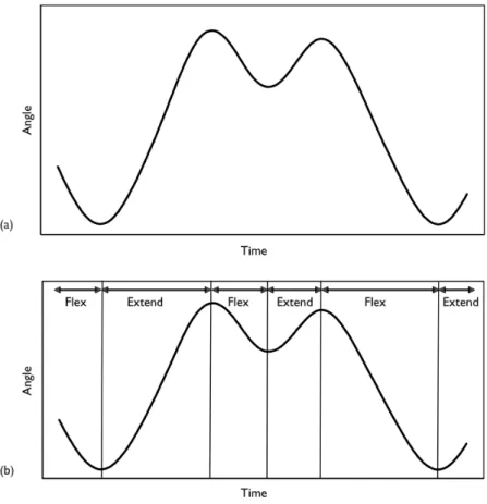
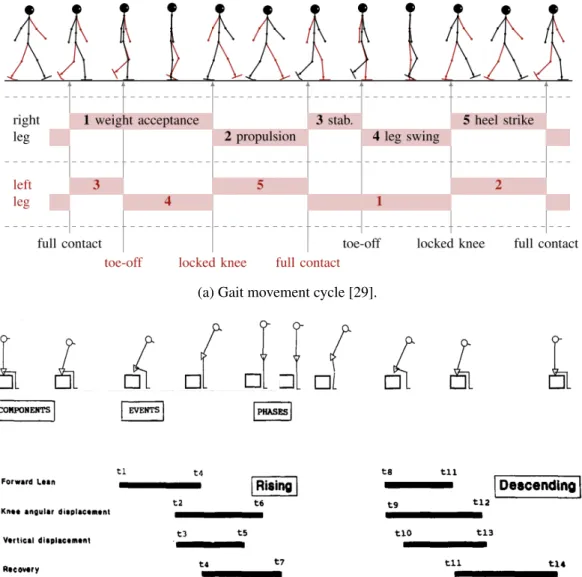
2.4 Examples of movement cycle diagrams... 12
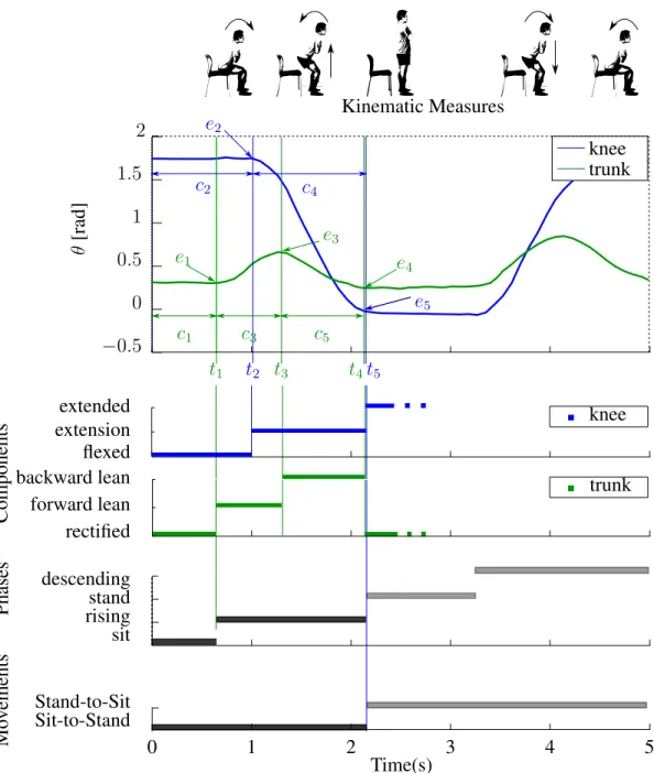
2.5 Movement description according to the definitions of events, components phases and movements. Each event (e) instant is marked with an arrow. For the knee angle there are two events (e2, e5): beginning and end of knee extension, which are also marked at t2 and t5. The interval between two events are the components (c) which are marked by double arrows. Events e2 and e5 form the component c4. The events and components for the trunk tilt angle are defined analogously: there are three events e1, e3 and e4 which are marked with arrows at t1, t3 and t4, forming three components c1, c3and c5. Rising phase starts at with e1and ends with e5. Sit phase and rising phase makes the sit-to-stand movement. ... 14
2.6 Estimation tasks... 17
2.7 Graphical representation of a Hidden Markov Model. ... 20
2.8 Graphical representation of a Linear Dynamic Systems. ... 24
2.9 Graphical representation of a Switching Linear Dynamic System. ... 27
3.1 Workflow of measurement systems and feature extraction. ... 32
3.2 Example of the segmentation and the motor performance parameters extrac-tion tasks. (a) Segmentaextrac-tion task: to determine the beginning and end of each movement (movement period) of a Sequence of Mixed Movements: Sit-to-Stand, Arm Raise, Squat, Bow and Stand-to-Sit. If the sequence is not predefined, there is the additional sub-task of determining each movement type. This segmentation result was obtained with the proposed method. (b) Motor performance parameters extraction (peak trunk tilt, knee extension period and rising phase period) for the Sit-to-Stand movement. ... 34
LIST OF FIGURES x 4.1 SLDS model. One event and component are marked in the scalar model (sj1
t ). One movement, and one multidimensional symbol ( t) and its corresponding scalar symbols are also indicated. The result in this figure was obtained with the proposed method... 39 4.2 Block diagram illustrating the complete method. Particularly, data flow of
variables and important algorithms steps for the proposed approach are de-picted. ... 43 5.1 Training data set consisting of one execution of the Sit-Stand-Sit movement
cycle. Events (ei), components (ci) and the rising and descending phases are identified using black arrows and red vertical lines. ✓ and ˙✓ indicates angle and angular velocity... 49 5.2 Movement cycle extraction validation with the Switching Linear Dynamic
System (SLDS) model and the Finite State Machine with thresholds (FSM) model using datasets containing one movement execution with different ve-locities: Normal, Fast and Slow. Red vertical lines represent the beginning of each component in the hand segmented dataset (used as ground truth)... 51 5.3 Cross validation for the movement cycle extraction with the Switching
Lin-ear Dynamic System (SLDS) model and the Finite State Machine with thresh-olds (FSM) model using datasets containing a sequence of 5 Sit-Stand-Sit movements executed with normal velocity. Red vertical lines represent the beginning of each component in the hand segmented dataset (used as ground truth). ... 52 5.4 Cross validation for the movement cycle extraction with the Switching
Lin-ear Dynamic System(SLDS) model and the Finite State Machine with thresh-olds (FSM) model using datasets containing a sequence of 5 Sit-Stand-Sit movements executed with varied velocity. Red vertical lines represent the beginning of each component in the hand segmented dataset (used as ground truth). ... 53 8.1 Data for case study of elderly experiment. Each colored curve represents a
distinct execution. Examples from healthy elderly subjects used for param-eterization respectively for (a) trunk and (b) knee angle. Data from elderly subjects with limited mobility used for validation is shown respectively for (c) trunk and (d) knee angle... 70 9.1 Descrições de movimento. ... 83 9.2 Descrição de movimento de acordo com as definições de eventos (e),
LIST OF FIGURES xi 9.3 Diagrama de blocos do método proposto. ... 86
List of Tables
3.1 Comparison Between Previous Works and Proposed approach ... 35 6.1 Segmentation Results for the 5 times Sit-to-Stand(5STS) and Mixed Whole
Body Movements (MWB) data sets in intra and inter-subject validation. Re-sults are presented as a percentage (%) of correct movement type recognition (MT), correct transition detection(C), false negatives (FN) and false positives (FP), within an error bound (terror) ... 57 6.2 Motor Performance Parameters Extraction results for the proposed
algo-rithm. Three parameters ( maximum knee angular velocity, peak trunk tilt and rising phase duration) relevant to the Sit-to-Stand movement are ex-tracted for each subject both using a intrasubject and inter-subject model validation. The mean and std for each parameter are presented, as well as the estimation mean error and std in percentage. ... 58 7.1 Comparison of offline and online estimation of the trunk tilt angle during the
Sit-to-Stand movement. Results shown for each subject in the intra-subject validation. The mean and standard deviation (std) for the trunk tilt is pre-sented, as well as the estimation mean error and standard deviation (std) in percentage. The cases where there was a delay in the detection are also indi-cated. ... 66 7.2 Comparison of online and offline segmentation for the 5 times Sit-to-Stand
(5STS) and Mixed Whole Body Movements (MWB) data sets in intrasubject validation. Results are presented as a percentage (%) of correct transition detection (C), false negatives (FN) and false positives (FP), within an error bound (terror < 0.3s). ... 67 8.1 Motor Performance Parameters Extraction results for the proposed algorithm
to the Elderly Experiment (subjects with limited mobility, LM) of STS move-ment in validation. ... 71
Notation and Abbreviations
MOCAP - Motion Capture System IMU - Inertial Measurement Unit DTW - Dynamic Time Warping TUG - Timmed Up and Go (test) HMM - Hidden Markov Model ZVC - Zero Velocity Crossing LDS - Linear Dynamic Model DBN - Dynamic Bayesian Network FB - Forwards-Backwards
RTS - Rauch-Tung-Striebel
SLDS - Switching Linear Dynamic System ABI - Acquired Brain Injury
VE - Virtual Environment FSM - Finite State Machine FP - False Positive
FN - False Negative MT - Movement Type
CPG - Central Pattern Generator GUI - Graphic User Interface
List of Symbols
i.i.d. - Independent with identical probability distribution e- event
c- component p- phase m- movement
s- switching variable (scalar SLDS) S - set of symbols for s
S - family of sets of S
- switching variable (multidimensional SLDS) D - set of symbols for
D - family of sets of D
x- hidden state in state-space model (scalar)
x- hidden state in state-space model (multidimensional) A- state transition matrix (state-space model)
r - hidden state noise
Q- covariance of hidden state noise
y- observed measurement in state-space model (scalar)
y- observed measurement in state-space model (multidimensional) C - observation matrix state-space model
w- measurement noise
⇧- state transition matrix (HMM model)
↵- forward operator (forwards-backwards algorithm) - backwards operator (forwards-backwards algorithm) - combined operator (forwards-backwards algorithm) v - constant velocity parameter
xv ⌃- variance
J - smoother gain matrix RTS
J - set of joints/kinematic variables j '- mapping function S ! D
P - set of ordered pairs with movement period T - set of movement types ⌧
E - set of symbols s associated with end of movement C - cost function in the SLDS-Viterbi
T - period or time-series length L - lag in fixed lag smoother
1 INTRODUCTION
Human movement science is on the verge of a revolution. Portable, low-cost sensors are quickly making their way in everyday activities, providing measurements of human motion which were previously reserved to cumbersome laboratory equipments and procedures. The amount and availability of quantitative data on human movement will directly impact in many areas such as: sports, rehabilitation and human-machine interaction.
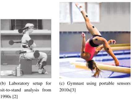
Human movement science, specifically biomechanics, has evolved alongside measure-ment devices, as illustrated in Figure1.1. Starting from the early works of photographic studies of Etienne-Jules Marey and Eadweard Muybridge in the 1880s, where sequences of photographs enabled qualitative understanding, description and assessment of human move-ments [4], passing on to the development of optical and wearable sensors in the 1980s and 1990s, which enabled quantitative measurements and therefore objective description, as-sessment and quantitative analysis [2]. But cumbersome setups limited the measurement of human movement to research settings. Today, the widespread of portable low-cost sensors have the potential to provide biomechanist and end users an unprecedented amount of quan-titative data of human movement [5, 6]. The interpretation and usage of these measurements are still an emerging field of study. Nonetheless, the deep understanding and advance us-age of these measurements are the cornerstone to unfold new techniques and procedures for human movement assessment.
It is a consent that feedback on movement execution from a qualified professional is ef-fective in performance improvement [7]. Moreover, during either in sports or rehabilitation sessions, incorrect execution of movements may lead to injuries or, at least, make the training session ineffective. Kinesiologists observe key features in movement execution and they rely on their knowledge to assess the quality of the execution of the movement. Based on this assessment and their experience they provide feedback to the subject with the goal of im-proving performance. Furthermore, the trainer is responsible for monitoring the evolution of the subject over time - based either on qualitative observations or quantitative measurements - to inspect the effectiveness of training.
Expertise in biomechanics is nowadays built on quantitative data and objective descrip-tions to gain scientific knowledge of how and why a movement is executed in a certain way [4]. In everyday practice, however, the kinesiologist will look at the movement executed by a subject and mentally execute a few tasks in order to assess the movement. First, even in a controlled environment, a movement is rarely executed alone, rather it is often part of a sequence of movements. The kinesiologist must mentally segment the sequence of
move-(a) Sequence of photographs from Etienne-Jules Marey circa 1880s
(b) Laboratory setup for sit-to-stand analysis from 1990s [2]
(c) Gymnast using portable sensors 2010s[3]
Figure 1.1: Evolution of human movement measurement devices.
ments to focus on the movement to be assessed. Second, inherent to segmentation, he must recognize which movement was executed. Next, once he is observing the desired movement, he will recognize critical attributes to evaluate the movement, for example: has a gymnast raised his arm high enough at the takeoff of a somersault? Has a patient leaned his trunk excessively forward during a sit to stand movement? Finally, the kinesiologist must monitor these critical attributes over many executions and training session to check for improvement. Portable sensors enhance observation, but assessment and monitoring are still carried out by the kinesiologist [8, 5].
The areas of augmented biofeedback and, more recently, telerehabilitation have gained much attention in the past few years because the literature shows that intensive practice schedules benefit acquisition and recovery and motor function [9, 10]. However, intensive practice schedules should be associated with supervised training for assessment, feedback and medium to long term monitoring, with the risk of running the session ineffective or event lead to injury. Professionally intensive supervised motor training sessions is not a realistic outlook in today’s scenario. The number of athletes or patients greatly outnumbers the number of qualified professionals. As a result, restricted time is spent in supervised training scenarios. Motion tracking combined with automatic assessment technology can assess and provide feedback to the user to correct the movement execution and monitor the progress over time. The advent of this technology can decrease the workload of trainers and offer the possibility of supervised personalized training sessions for a larger audience as well as releasing trainers to perform additional higher level evaluations and procedures.
Another area with potential application of automatic human movement assessment is the development of intelligent prosthesis. These electro-mechanical devices interpret the human movement and act to restore impaired functions of the body. Although some attention has been given to automatic human movement segmentation and assessment they are usually simple computational solutions developed specifically for each device and function restored [11].
Furthermore, the techniques presented in this thesis could also be applied to human-machine interactions. As more appliances are equipped with motion sensors, the area of multimodal interaction, i.e. interacting with machines through touch, speech and gesture, become more tangible. Multimodal interaction offers not only comfort and flexibility, but may open possibilities of human-machine interactions for individuals with impairments [12]. To summarize, much attention has been given to evidence-based objective movement description, motor control learning with augmented feedback and telerehabilitation. Like-wise much attention has been given to portable and low-cost sensor technology for human movement measurements. In contrast, little attention has been given to automatic movement assessment. The reason is that automatizing tasks seemly easy for humans - such as recog-nizing movements, determining the start and end of a movement and observe key features of the movement to judge its quality - requires from one side deep understanding of human nature of the tasks to be automatized and from another side advanced mathematical mod-els and complex machine learning techniques. In this thesis we automatize the process of segmentation, movement type recognition, and assessment.
The main contributions from this thesis can be summarized as:
1. Unified mathematical approach for automatic segmentation, movement type recog-nition and motor performance parameters extraction: different from previous works in the literature, we use the same mathematical modeling and estimation procedures to solve the required tasks for automatization of human assessment. This simplifies software implementation, model parametrization and application of the method to any type of movement described by kinematic parameters.
2. Parametrization procedures that require no background in signal processing: our proposed method uses manually labeled data sets to automatically parametrize the mathematical models. Therefore professionals with no background in signal process-ing may directly use our proposed framework without the need to understand the un-derlying mathematics.
3. Implementation and validation on diverse experiments: we implemented our method and tested under different conditions with varied population to showcase performance
and applicability.
This manuscript is organized as follows: Chapter 2 provides the reader with the neces-sary theoretical background from both human movement analysis and stochastic modeling and estimation to understand the framework proposed in this thesis. Next, in Chapter 3, the recent developments in automatic human movement segmentation and assessment are presented. Then, in Chapter 4, the proposed framework for using switching linear dynamic system modeling for automatic human movement segmentation and assessment is presented. Following, four case studies are presented to showcase the features of the proposed frame-work. In Chapter 5 a movement cycle diagram is obtained with the proposed framework and compared with an heuristics approach. In Chapter 6 a multivariate case is used to accomplish segmentation, movement type recognition and motor performance parameters extraction, the processing is done offline. In Chapter 7 an online variation of the proposed framework is used for online segmentation and motor performance parameters extraction. To conclude the case studies, in Chapter 8 the framework is used to extract motor performance parameters from a database collected from elderly subjects. Finally overall conclusions and outlooks are presented in Chapter 9.
2 THEORETICAL BACKGROUND
2.1 IMPORTANCE OF HUMAN MOVEMENT ANALYSIS
Kinesiology is the science of human movement. Biomechanics is a sub-discipline of kinesiology that involves precise description of human movements and the study of the me-chanics that causes the movement [7].
The study of biomechanics is relevant to professional practice in many kinesiology pro-fessions. In everyday practice an athletic trainer or rehabilitation therapist rely on mea-surements or visual observations to analyze the movement execution. They count on their experience (on biomechanics) to pay attention to certain aspects of the movement at particu-lar moments. Based on these observations and background knowledge the coach or therapist may infer the causes of this poor execution due to lack of technique or impairment.
The role of most kinesiology professionals is to prescribe technique changes and give instructions that allow a person to improve performance. Either for athletes to advance their technique or patient to enhance or restore movement capability.
The reason of any assessment is to enable a positive decision about a physical movement. An athletic trainer might check if a variation of a technique will minimize the mechanical energy required for a certain movement. An orthopedic surgeon may wish to observe im-provements in knee strength of a patient a month after surgery. A basic researcher may wish to interpret the motor changes due to controlled perturbation to verify or negate different neural control theories [4].
Human movement assessment falls on a continuum between qualitative and quantitative. Quantitative analysis requires the measurements of biomechanics variables and usually re-quires electronic sensors and computer processing. Even short movements may result in thousands of samples of data to be collected, scaled and numerically processed. On the contrary, qualitative analysis is defined by [7] as: "systematic observation and introspective judgment of the quality of human movement for the purpose of providing the most appropri-ate intervention to improve performance".
Numerical measurement systems enable precise observations of what may escape the eyes. The advantages of quantitative over qualitative assessment are: accuracy, consistency and precision. Besides, it provides a mean for objective comparison. Moreover, the use of numerical measurement systems allows the establishment of baseline values for variables associated to different movements.
(a) Stick figure of the sit to stand movement [15]. (b) Plot of time-series of angle joint in a gym-nastics movement [16].
Figure 2.1: Descriptions of movements.
These advantages comes at cost and complexity, as a result most quantitative biome-chanics analysis is performed in research settings. However, in recent years there has been an increase in low-cost, commercially available and easy to use devices to measure biome-chanics variables [13, 14, 7].
As strongly emphasize by [4], "the scientific approach to biomechanics has been charac-terized by a fair amount of confusion". It is common to find misused terms in the literature when reporting studies. Descriptions of human movement are often referred to assessment and studies containing only measurements have been falsely passed on as analysis, to cite two recurring examples. Consequently, these terms must be clearly defined.
Measurements are the quantities provided by the sensors (although post-processing may be required) for each biomechanics variable.
Descriptions are forms of representing measurements to facilitate assessment. They can take the graphical form such as: time-series plots, movement cycle diagrams or stick-diagrams such as depicted in Figure 9.1. Or they can be a mathematical formula that results in an outcome measure such as: gait velocity or maximum heigh of a jump. Throughout this thesis outcome measures will be referred to as motor performance parameters.
Assessment is the act of evaluating, i.e. estimating or judging the value of a variable. To monitor means to perceive changes over time. A coach may monitor the improvement of technique from an athlete, while a therapist may monitor the rehabilitation of a patient. Monitoring, however, does not inform why improvement (or lack of) happened, it merely documents changes over time.
To analyze is to examine the movement carefully and in detail so as to identify causes, key factors and possible outcomes.
Baseline valuesand descriptions are important tools for assessment and analysis of human movements in sports and healthcare.
In sports, for example, [16] investigates the ideal timing and angle variability in a com-plex gymnastics whole body movement with the goal of achieving consistent performance. Measurements are described using a movement cycle diagram to compare the differences between successful and unsuccessful executions. As another example, [17] monitors certain motor performance parameters of the rowing movement during a low intensity high volume training session to check if decline in the technique over this period.
In healthcare, for example, in [18], the authors investigate the gait pattern of patients suffering from Parkinson’s disease and compare it to gait patterns of a healthy control group. Another study, [19], compares the gait pattern in Parkinson’s disease patients on an off med-ication to establish the benefits of treatment.
The same type of analysis has gained attention in the last decades for the Sit-to-Stand movement. Early works on definitions and normative data presentation, such as [20, 21], provided the basis for studies on the deviations of this movement influenced by various con-ditions. For example, the work in [22] uses the Sit-toStand movement to investigate motor control and stability limitations on hemiplegic patients. Another study, [23], investigates the changes in strategies to execute the Sit-to-Stand due to obesity. Deviations of kinemat-ics in frail elderly subjects when compared to healthy subjects make it possible to detect frailty and monitor the success of a rehabilitation program [24]. The success of a rehabilita-tion program for patients recovering from total knee arthroplasty can also be assessed using kinematic measurements during the Sit-toStand movement, such an example is presented in [25].
These are just a few examples from a vast literature on the recent developments using standardized and uniform descriptions for human movement measurements. Furthermore it indicates the relevance of studies in automatic human movement analysis and its potential applications.
2.2 HUMAN MOVEMENT MEASUREMENTS
Human movement measurement is a form of observation, through the use of devices, to describe phenomena in terms of variables to be analyzed. Data acquired from measurement
systems may elucidate motor impairments after trauma or elucidate effects of controlled external intervention [26]. They are used to describe, characterize, measure the impact of external factors and analyze human movement. Kinematic and kinetic data may be combined and analyzed to explain movement features. Besides merely describing the movement, this process helps explain why a movement is executed in a particular way.
Along with the quality of the measurements, an important factor to consider in the choice of measurement devices for clinical application is the complexity in the measurement setup. Aspect such as: will the patient need to undress, are there markers to be placed, has the mea-surement device limited area coverage, among others need to be weighted when choosing a measuring device or setup[26].
In human movement studies there are mainly three types of measurement variables: time, kinematic and kinetic. Time may be used alone to measure the duration of a certain move-ment, but it provides more information when associated with a kinematic or kinetic variable. Kinematic variables describe the movement of the body, they are either linear (displacement, velocity and acceleration) or angular (displacement, velocity and acceleration). Kinetic vari-ables are either the force or force moment that generates the movement[26].
The devices considered gold standard for both linear and angular kinematic measure-ments are the infra-red marker-based multi-camera motion capture systems (MOCAP) from manufactures such as Vicon1or Qualisys2. Electronic goniometers, such as Biometrics3, are also gold standard measurement devices for only angular kinematic variables.
In recent years, there has been a constant development in low cost portable measurement devices for human movement. These devices are expected to make their way into clinics and homes to monitor movements from recovering patients during treatment or athletes in sport sessions [5] [27] [6][28].
Kinematic measures can be obtained with markerless optical-based MOCAP, such as the Microsoft Kinect 4 or Asus Xtion 5. Coupled with dedicated software, they provide measurements in space representing the joints of a skeleton model for the human body. With these coordinates, it is possible to reconstruct the pose in terms of the linear and angular kinematic variables at each time frame. These vision-based devices have the advantage that no device needs to be attached to the user. But on the downside, they have a relative small coverage area, which limits the range of linear displacement. Also the software is made for
1http://www.vicon.com/System/Bonita 2http://www.qualisys.com
3http://www.biometricsltd.com/gonio.htm 4https://dev.windows.com/en-us/kinect
(a) Qualisys Marker-based Multi-camera MOCAP.
(b) Delsys Trigno IMU System. (c) Microsoft Kinect Markerless Optical MO-CAP.
Figure 2.2: Different MOCAP Devices. stand up poses, movements with hip flexion are not well measured.
Another type of low cost MOCAP devices are the ones based on multiple inertial mea-surement units (IMU), such as Delsys6, Yei7or XSens8. IMUs provide the angular orienta-tion in reference to an absolute coordinate system. The reconstrucorienta-tion of angular kinematic data is done using a skeleton model of the human body. The advantage of IMU based mea-surement systems (compared to optical based) is the larger coverage area, which provides the user with more linear displacement. Although it is possible to estimate linear kinematic variables, the result is usually very inaccurate and degenerates with time. Therefore this type of MOCAP system is used to obtain only angular kinematic measurements. Another
6http://www.delsys.com/products/wireless-emg/
7
https://www.yostlabs.com/yost-labs-3-space-sensors-low-latency-inertial-motion-capture-suits-and-sensors
disadvantage is the need to place multiple sensors in various body parts. Figure 2.2 shows examples of MOCAP devices.
As for kinetic variables, the most popular gold standard device is the force platform, such as Bertec9. Although stand alone force transducers also provide accurate and precise measurements, they require a dedicated physical structure to be mounted on, which limits their flexibility for different movement types.
A low cost option to obtain kinetic data is the Nintendo Wii Board10. This device uses sensors to estimate the resultant force applied in the board and its center of pressure, but not the orientation, as in the gold standard force platform.
Finally electromiography (EMG) signals are not kinematic or kinectic measurements, but they measure the muscle activity that causes human movement and are usually associated to kinematic or kinetic data in human movement analysis. Deslsys Trigno system is also able to provide EMG measurements, along with IMU data. Although not dealt with in this thesis, kinetic and EMG could be processed with the framework presented herein.
2.3 ASSESSMENT OF KINEMATIC AND KINETIC DATA
When kinematic or kinetic data is indexed with time, the result is a time-series of kine-matic or kinetic measurements. The most common tool to analyze these time-series are the resulting graphs [1], because it is easier to visualize the movement pattern. The slope and curvature of the time-series graph indicate key features of a movement execution and pro-vide a powerful tool for movement analysis. Figure 2.3 shows the angular displacement of the knee during one gait cycle on a treadmill. Analyzing the slopes and inflection points, it is possible to determine the beginning and end of each flexion or extension for this particular joint.
An extension of kinematic time-series graphs are the movement cycle diagrams [20]. Starting from the premiss that the same movement executed by different individuals will have a similar pattern and based on standardized and uniform definitions, time-series mea-surements of kinematic and kinetic data can be annotated for quantitative performance infor-mation extraction. Gait cycle diagrams are one of the most common example. Gait analysis is a well established field of study, mainly due to the use of the gait cycle diagram as a tool to describe, report and compare gait performance across different research findings (also due to the importance of gait movement). Because of the success of the gait cycle diagram,
re-9http://bertec.com/products/force-plates/ 10http://wiifit.com
Figure 2.3: Time-series of knee angle measurements from a subject walking on a treadmill and the indication of changes in slope. Adapted from [1].
searchers have also proposed standardized descriptions for other movement types, such as the Sit-Stand-Sit movement [20] and also sport activities [1]. Figure 2.4 shows the move-ment cycle diagrams for gait and sit-to-stand-to-sit movemove-ments. Different kinetic and kine-matic variables are used to determine the key moments used to describe each phase of the movement, so the generation of the movement cycle diagram usually requires multivariate measurement time-series.
In this section, we present the concepts and formal definitions from human movement analysis that are used to generate a movement cycle diagram and are the basis of our pro-posed method in Chapter 4. This includes definitions of what is considered a single move-ment entity and how we describe each movemove-ment in order to extract relevant spatiotemporal quantitative information in the scope of our study.
We delimit our study to a class of movements defined by [31, 32] as discrete movements. It is defined by [32] as: “a movement that has an unambiguously identifiable start and stop; discrete movements are bounded by distinct postures”. An example of a discrete movement is standing from a chair: the start is marked by the siting posture and the stop is marked
(a) Gait movement cycle [29].
(b) Sit-Stand-Sit movement cycle (adapted from [20, 30]).
Figure 2.4: Examples of movement cycle diagrams.
by the standing posture. The movements used in the related works [33, 34] strictly fall in this class of movements. Throughout our work, the reference to one movement will refer to the motion executed between two postures. This distinction is made at this stage to restrict the scope of our work and avoid comparisons with methods that require a cyclic movement, such as the algorithms presented in the review [35]. But since our proposed method is in-spired in the generation of the movement cycle diagrams, it can be used also to describe cyclic movements. However, we do not make any assumption about the cyclic nature of the movement.
One way to systematically describe one movement is to break it down into elements according to the change in the slope of kinematic and/or kinetic time-series, such as flexion and extension, of each body joint and its effects in posture changes.
We take the following definitions used by [20] to systematically describe discrete move-ments:
• Events (e) is a single identifiable occurrence of a change in the trend of the recorded movement pattern for each kinematic or kinetic variable.
• Components (c) are defined as those constituent parts of the movement, that are bounded by events within the same variable.
• Phases (p) are build from components and are also bounded by events, but the bound-aries can be established using events from different variables.
• Movement (m) is a sequence of one occurrence of all phases between two distinct postures..
To clarify the meaning of these definitions, we take for example a sequence of two dis-crete movements: sit-to-stand and stand-to-sit shown in Figure 9.2. The kinematic mea-surements used to describe these movements are the knee angle and trunk tilt angle. The sit-to-stand movement is described in detail.
A movement cycle diagram displays the duration of each component of both the knee an-gle and the trunk tilt anan-gle. The rising phase, as defined by [20], starts with the forward lean of the trunk and ends either with the full knee extension or full trunk extension, whichever occurs first. In our work the sit-to-stand movement is described with two phases: quiet siting and rising phase. The movement ends when the person reaches a full upright position. In a similar matter, the phases for the stand-to-sit movement are defined. The duration of each phase for both the sit-to-stand and the stand-to-sit movements are shown in a diagram in Figure 9.2, as well as the duration of each movement.
2.4 MATHEMATICAL BACKGROUND
This section provides the reader the basic concepts and a brief theoretical background on the mathematical representation and the estimation theory to be addressed in this thesis. We begin by recalling basic stochastic system concepts using state-space models and most common algorithms associated to filtering, smoothing and prediction. Particularly, we are interested in introducing the reader the concepts regarding switching linear dynamic systems. For readers unfamiliar with stochastic systems or estimation theory, the general idea behind switching linear dynamics systems (SLDS) follows from combination of hidden Markov models with Kalman filtering for linear systems.
Time(s) 0 1 2 3 4 5 ✓ [rad] e1 e2 e5 c3 c5 c4 Kinematic Measures 0.5 0 0.5 1 1.5 2 e4 e3 t3 t4 t2 t5 c2 c1 Mo vements Phases Components knee trunk sit risingstand descending Sit-to-Stand Stand-to-Sit rectified forward lean backward lean flexed extensionextended t1 knee trunk
Figure 2.5: Movement description according to the definitions of events, components phases and movements. Each event (e) instant is marked with an arrow. For the knee angle there are two events (e2, e5): beginning and end of knee extension, which are also marked at t2and t5. The interval between two events are the components (c) which are marked by double arrows. Events e2 and e5 form the component c4. The events and components for the trunk tilt angle are defined analogously: there are three events e1, e3and e4which are marked with arrows at t1, t3 and t4, forming three components c1, c3 and c5. Rising phase starts at with e1and ends with e5. Sit phase and rising phase makes the sit-to-stand movement.
Using hidden Markov models (HMMs), we are able to decode a sequence of discrete states—usually, discrete and finite—but we are unable to track the continuous values be-tween the states. Think of it as a sequence of photographs, where we can estimate the sequence of poses that generated that sequence of photographs but we are unable to describe the movements between poses using a simple HMM. In contrast, the Kalman filter (KF) suc-cessfully tracks continuous linear movements over time—for instance, the KF can be used to track a particular body motion. We can think of an observer following the movement in a recorded film. However, only one model is used to represent the movement and this model is linear—consequently the Kalman filter can only track one simple and limited movement at a time. Moreover, since it is based on a single model, the technique is not suitable to segment a sequence of movements.
A switching linear dynamic system (SLDS), in essence, combines a hidden Markov model with Kalman filtering. So we can think of the basic elements of the SLDS as short movie of simple movements between two poses. By combining the sequence of these basic elements, we can represent a considerably more complex and complete movement. Since we know which set of basic elements are used to represent each movement, we can also use it to segment and recognize a sequence of movements in a given film and breakdown each movement to analyze critical poses or transitions.
In the light of this discussion—and, in contrast to the characteristic of existing movement analysis techniques—this thesis addresses and exploits the SLDS modeling in the develop-ment of the novel framework for movedevelop-ment analysis. In this sense, the mathematical de-velopments presented in this section concerning SLDS provide the necessary background to fully understand the ideas and results that follows throughout the thesis and how the SLDS model fitting is employed in the context of movement analysis. Hence, readers are encour-aged to read the whole section, even if they are already familiar to the notions and concepts presented herein.
2.4.1 State-Space Models
The state-space framework is a mathematical model used to represent a dynamic physical system based on a set of input, output and state variables related by first-order differential or difference equations. To abstract from the number of inputs, outputs and states, these variables are expressed as vectors which evolves over a time t based on a function f(·). The output of the system can be the state itself or a function of the state and input variables, that
is,
˙x(t) = f (t, x(t), u(t)), y(t) = h(t, x(t), u(t)),
where x, y, and u denote the state, output and input vectors, and x(0) defines the initial condition of the system. In the particular case where the dynamic system can be described by linear finite-dimensional invariant equations, the differential equation can be described in matrix form by
˙x(t) = Ax(t) + Bu(t), y(t) = Cx(t) + Du(t),
where the matrices A, B, C, D are known constant matrices that defines the dynamics of the system. In addition, throughout this manuscript, the dynamic system is assumed to be a sampled-based system where data is acquired at fixed intervals—sample time T . The evolution of a causal11linear state-space system can therefore be described by
xk+1 , x (T(k + 1)) = Axk+ Buk, yk = Cxk+ Duk,
where xk, yk and ukdenote the state, output, and input vectors of the system at instant kT . It is important to highlight that in more realistic scenarios, this model may not be per-fectly accurate since the system dynamics is usually influenced by random noises and model uncertainties. Indeed, in practical applications, not only the dynamics of the system may be influenced by uncertainties and noises but the measurement process itself is liable to sensor errors and inaccuracies. To improve the estimation, tracking and control of the desired vari-ables of interest, it is essential to address the disturbances as neglecting their influence would most likely lead to poor performance. In this case, the state and output variables xk and yk become random variables [36] and the system description becomes
xk+1 = Axk+ Buk+ rk, yk= Cxk+ Duk+ wk,
where rk and wkdescribe the system dynamics noise and the measurement noise. Through-out this thesis, we will assume that both noises are defined as Gaussian white noise, that is, they can be regarded as a sequence of uncorrelated Gaussian distributed random vari-ables with zero mean and finite variance where the samples are independent with identical probability distribution (i.i.d.) [36].
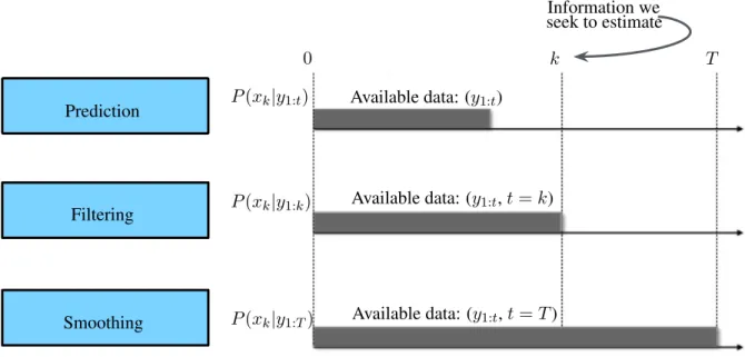
Prediction Filtering Smoothing P (xk|y1:t) P (xk|y1:k) P (xk|y1:T) 0 k T Information we seek to estimate Available data: (y1:t) Available data: (y1:t, t = k) Available data: (y1:t, t = T )
Figure 2.6: Estimation tasks.
In this thesis, we are particularly interested in analyzing a time-series of human move-ments measuremove-ments. This analysis can be done online where a new estimation is performed at each interaction—as soon as a new data is available—or offline where the analysis is performed only after the whole dataset is available.
The main advantages of the state space representation over related methods are: they can easily represent multivariate systems, they can easily incorporate prior knowledge and they do not suffer from finite window effect (frequency based models, such as the Fourier transform, are sensitive to sampling window during discretization) [37].
2.4.2 Estimation tasks in State-Space Models
To properly describe and estimate human movement, we are mainly interested in three estimation tasks based on a sequence of readings: prediction, filtering and smoothing, as illustrated in Figure 2.6. Additionally, in case that the state space is discrete—that is, con-sidering only a discrete and usually finite set of data—there is also the task of estimating the most likely sequence of x that generated the observations y.
• Prediction: estimation of a future state, that is, to calculate the posterior probabil-ity distribution for a future state k, given all the observations up to the moment t: p(xk|y1:t), 0 < t < k.12
12Throughout the manuscript the notation y
• Filtering: estimation of the current state, that is, to calculate the posterior probability distribution for the present state k, given all the observations up to the moment k: p(xk|y1:k).
• Smoothing: estimation of a past state, that is, to calculate the posterior probability distribution of an earlier state k, given all observations up to the moment T : p(xk|y1:T), 0 < k < T.
• Viterbi Decoding: estimation of the most likely sequence of states that generated the sequence of observations: argmaxx1:kP (x1:k|y1:k).
It is important to highlight that the above estimation tasks—as described—depend on whole available dataset. Hence, a large enough number of readings yields in soaring com-putational costs. Indeed, as k ! 1, the estimation costs becomes unfeasible. To avoid soaring expenses, most estimation algorithms are based on stochastic process satisfying the Markov property. A stochastic process has the Markov property if the conditional probabil-ity distribution of future states of the process depends only upon the present state, not on the sequence of events that preceded it [38].
If the unknown—herein, we can also called hidden—state variable x is continuous—for instance, if x 2 R—we have a stochastic linear dynamic system (LDS). On the contrary, if x can assume solely a discrete set of values, we have a hidden Markov model (HMM) [39],[40],[41].
Filtering and Prediction The most common inference problem in online analysis is to recursively estimate the belief current state using Bayes’ rule (see [42] for further informa-tion): P (Xt|y1:t)/ P (yt|Xt, y1:t 1)P (Xt|y1:t 1) = P (yt|Xt) " X xt 1 P (Xt|xt 1)P (xt 1|y1:t 1) #
Using the Markov property, the problem can be considerably simplified by replacing P (yt|Xt, y1:t 1)with P (yt|Xt). Similarly, the one-step ahead prediction, P (Xt|y1:t 1), can be computed from the prior belief state, P (Xt 1|y1:t 1), because of the Markov assumption on Xt.
Therefore, based on the Markov assumption and its implications, recursive estimation consists of two main steps: predict and update. The predict step regards the estimation of
P (Xt|y1:t 1), sometimes written as ˆXt|t 1. Updating the expected mean value yields on com-puting P (Xt|y1:t), sometimes written as ˆXt|t. Once we have computed the prediction step, we can disregard the previous belief state: this operation is often called "rollup". Hence, the overall procedure takes constant space and time—which in turn implies time indepen-dence —per time step. This task is traditionally called "filtering", because we are filtering out the noise from the observations. However, in some cases the term tracking might also be employed when considering the dynamic filtering of a given variable.
Smoothing In opposite to the prediction and filtering, the smoothing task takes the whole dataset—that is all the information up to the current time T—to estimate a given state of the past, that is, compute P (Xt l|y1:T), where l > 0 is the lag variable that defines the size of the smoothing variable and l < t < T . This is traditionally called fixed-lag smoothing. Considering offline estimation, we can also consider all data up to the time t. This is called fixed-interval smoothing and corresponds to computing P (Xt|y1:T)for all 1 t T .
Viterbi Decoding Within Viterbi decoding (or computing the "most probable explana-tion"), the goal is to compute the most likely sequence of hidden states given the data, that is x⇤
1:t = argmaxx1:tP (x1:t|y1:t). Note that this is a different task than smoothing where only
the most likely (marginal) state is estimated at each time t, as will be made clear in Section 2.4.3.3.
2.4.3 HMM 2.4.3.1 Model
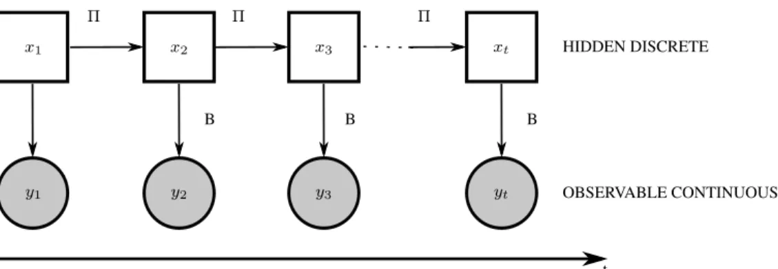
A Hidden Markov Model (HMM) is a random variable automaton [41]. The discrete hidden state x(t) (the random variable Xt ) belongs to a discrete (usually finite) set Xt 2 {1, . . . , S}. The observation y(t) (the random variable Yt) may also belong to a discrete (usually finite) set Yt 2 {1, . . . , L}, or it may be a continuous Gaussian distribution. The HMM model contains: a distribution for the initial state ⇡t=0(s) = P (X0 = s); a transition model ⇧, where ⇧ is a stochastic matrix, which means that each element (i, j) represents the probability of transition from state i to state j at the instant t, i.e. ⇧(i, j) = P (Xt = j|Xt 1 = i); and an observation model, which can also be a stochastic matrix B(y, i) = P (Yt = y|Xt = i), in the case that Yt is discrete. In the case that Yt is continuous, the observation model will be a set of Gaussians P (Yt = y|Xt = i) = N (y; µi, ⌃i), where µi represents the mean and ⌃i variance..
In an equivalent form, the HMM model can be written as
P (xt|xt 1) = xTt⇧xt 1, with (2.1) yt = B(yt, xt)
P (x0) = ⇡0
where xt is a 1 ⇥ S unit vector that indicates the index of the value xt from the set Xt 2 {1, . . . , S}. Figure 2.7 is a graphical representation of the evolution of a HMM in (2.1).
⇧ x1 x2 y1 y2 B x3 y3 xt yt t HIDDEN DISCRETE OBSERVABLE CONTINUOUS ⇧ ⇧ B B
Figure 2.7: Graphical representation of a Hidden Markov Model.
The two most common tasks when using a HMMs are smoothing, which is usually done by the forward-backward algorithm, and estimation of the most likely sequence, which is done by the Viterbi algorithm [41].
HMMs are also widely used in many applications, such as speech recognition and sensor fault detection. In speech recognition Viterbi decoding is used to infer the sequence of letters of the spoken word from pre-processed audio measurements [43]. In fault sensor detection smoothing or filtering is used to check if the sensor readings are coherent with its expected behavior and operation limits [41].
2.4.3.2 Inference with Forwards-Backwards
Offline smoothing can be performed in an HMM using the well-known forwards-backwards algorithm (FB) [43]. In smoothing the whole observation dataset yt, t = 1 : T is available. Similar to filtering, the forwards-backwards algorithm uses prediction and update to estimate xtbased on yt. However, it first predicts and updates xtwith the observations yt, t = 1 : T in the forwards pass. Next it refines the estimates of xtgoing back in the observation dataset yt, t = T : 1in the backwards pass. Finally both the forward and backwards estimates are combined to get the estimates of each xt based on the whole available observation dataset yt...
The basic computation of the FB algorithm is to first recursively calculate, in the forwards pass from t = 1 : T , the forwards operator ↵t(i)defined as:
↵t(i), P(Xt= i|y1:t)
Next, in the backwards pass from t = T : 1, the backwards operator t(i), defined as: t(i), P(yt+1:T|Xt= i)
is recursively calculated. Finally they are both combined to produce the combined operator t, defined as:
t(i), P(Xt= i|y1:T) to calculate the final estimate of each xt.
The term t(i), P(Xt = i|y1:T)can be expanded using Bayes rule, which results in: P (Xt= i|y1:T) =
1 P (y1:T)
P (yt+1:T|Xt= i)P (Xt= i|y1:t) but ↵t(i), P(Xt = i|y1:t)and t(i), P(yt+1:T|Xt = i), therefore:
t/ ↵t.⇤ t
where .⇤ denotes element wise product, i.e. t(i) / ↵t(i) t(i). In Sections 2.4.3.2 and 2.4.3.2 we will explain how to compute ↵tand t.
The forward pass To compute ↵trecursively in the forward pass, first we must elaborate the following equations: starting from the definition
↵t(j), P(Xt = j|y1:t) = 1 ct P (Xt = j, yt|y1:t 1) where P (Xt= j, yt|y1:t 1) = " X i P (Xt= j|Xt 1= i)P (Xt 1= i|y1:t 1) # P (yt|Xt = j) and ct= P (yt|y1:t 1) = X j P (Xt= j, yt|y1:t 1)
what ctrepresents is the probability of the sequence of observations. In most cases it is just considered equal to one because the observations are taken as true.
Since the computation starts at t = 1, the equations are reduced to ↵1(j) = P (X1 = j|y1) =
1 ct
or in the vector-matrix notation, this becomes
↵1 / B⇡0
where B comes from the HMM model, and ⇡0 is given. For each next time step, from t = 2 : T, ↵tcan be calculated as:
↵t / B⇧T↵t 1
where ⇧T denotes the transpose of ⇧ (from the HMM model).
The backwards pass To compute tin the backwards pass, we start at the end of the ob-servation dataset, t = T . Since we have reached the end, P r(yT +1:T|XT = i) = P r(;|XT = i) = 1and therefore:
T(i) = 1 The recursive step is then:
P (yt+1:T|XT = i) = X j P (yt+2:T, Xt+1= j, yt+1|Xt= i) = X j P (yt+2:T|Xt+1 = j, yt+1, Xt= i)P (Xt+1= j, yt+1|Xt= i) = X j P (yt+2:T|Xt+1 = j)P (yt+1|Xt+1= j)P (Xt+1 = j|Xt= i) or using the vector-matrix notation:
t= ⇧B t+1 2.4.3.3 Inference with Viterbi
The target of Viterbi decoding (or computing the "most probable explanation"), is to find the most likely sequence of hidden states given the observation data:
x⇤1:t = argmaxx1:tP (x1:t|y1:t)
By the Bellman’s principle of optimality, the most likely path to reach xt consists of the most likely path to some state at t 1, followed by a transition to xt. Hence we can compute the overall most likely path as follows. Similarly to the forwards-backwards algorithm, we introduce an operator, t, for recursive computation:
In the forward pass, starting from the first observation and moving towards t = T , we compute
t(j) = P (yt|Xt= j)maxiP (Xt= j|Xt 1 = 1) t=1(i).
This is analogous to the forwards pass of filtering, except we replace the sum with the cor-responding maximum value. In addition we keep track of the identity of the most likely predecessor to each state:
t(j) = argmaxiP (Xt= j|Xt 1 = i) t 1(i)
In the backwards pass, we can compute the identity of the most likely path recursively as follows:
x⇤t = t+1(x⇤t+1).
Viterbi decoding is different from forwards-backwards algorithm because it maximizes all the transitions xt 1 ! xtin the sequence resulting in the most likely path x⇤t=1:T, whereas forwards-backwards finds only the most likely (marginal) state xtat each time t.
2.4.4 Linear Dynamic Systems 2.4.4.1 Model
In a Linear Dynamic System (without inputs) we assume that the random variables Xt2 RNx, Y
t 2 RNy and that the transition of the hidden state xtand observation ytat each time interval are linear Gaussian in the form:
P (Xt= xt|Xt 1= xt 1) = N (xt; Axt 1+ µX, Q) (2.2) P (Yt= yt|Xt= xt) = N (yt; Cxt 1+ µY, R)
Equations (2.2) can be written in the vector-matrix form, which is more recurrent in the literature:
xt+1 = Axt+ rt+1 (2.3)
yt = Cxt+ wt
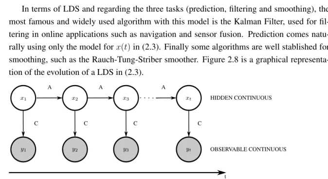
where xt 2 RN is the hidden state of the state-space model, rt (r ⇠ N(0, Q) is the state noise, yt 2 RM is the observed measurement of the system, wt (w ⇠ N(0, R) is the measurement noise. A is the state transition matrix and C is the observation matrix. The form in (2.3) is widely used in estimation and control theory.
In terms of LDS and regarding the three tasks (prediction, filtering and smoothing), the most famous and widely used algorithm with this model is the Kalman Filter, used for fil-tering in online applications such as navigation and sensor fusion. Prediction comes natu-rally using only the model for x(t) in (2.3). Finally some algorithms are well stablished for smoothing, such as the Rauch-Tung-Striber smoother. Figure 2.8 is a graphical representa-tion of the evolurepresenta-tion of a LDS in (2.3).
A x1 x2 y1 y2 C A x3 y3 A xt yt C C t HIDDEN CONTINUOUS OBSERVABLE CONTINUOUS C
Figure 2.8: Graphical representation of a Linear Dynamic Systems.
2.4.4.2 Inference with Kalman Filter and RTS Smoothing
The equations for Kalman filtering / smoothing can be derived in an analogous manner to the equations for HMMs, except the algebra is somewhat heavier.
Forwards pass (Kalman Filter) Let us denote the mean and covariance of the belief state P (Xt|y1:t)by (xt|t, ⌃t|t). The forward operator,
(xt|t, ⌃t|t, Lt) = F wd(xt 1|t 1, ⌃t 1|t 1, yt; At, Ct, Qt, Rt) is defined as follows. First, we compute the predicted mean and variance
xt|t 1 = Axt 1|t 1
⌃t|t 1 = AVt 1|t 1A0+ Q
Then we compute the error in our prediction (the innovation) et, the variance of the error St, the Kalman gain matrix Kt, and the conditional log-likelihood of this observation Lt:
et = yt Cxt|t 1 St = C⌃t|t 1C0+ R Kt = Vt|t 1C0St1
Finally, we update our estimates of the mean xt|tand variance ⌃t|t: xt|t = xt|t 1 + Ktet
⌃t|t = (I KtC)Vt|t 1 = Vt|t 1 KtStKt0
These equations are more intuitive than they may seem. For example, our expected belief about xt is equal to our prediction, xt|t 1, plus a weighted term, Ktet, where the weight Kt= ⌃t|t 1C0St 1, depends on the ratio of our prior uncertainty, ⌃t|t 1, to the uncertainty in our error measurements St.
Backwards pass (RTS Smoothing) The backwards operator is defined as follows: (xt|T, ⌃t|T, ⌃t 1,t|T) = Back(xt+1|T, ⌃t+1|T, xt|t, ⌃t|t; At+1, Qt+1)
this is the analog of the recursion in Section 2.4.3.2. First we compute the following predicted quantities (or we could pass them in from the filtering stage):
xt+|t = At+1xt|t
⌃t+1|t = At+1⌃t|tA0t+1+ Qt+1 then we compute the smoother gain matrix
Jt = ⌃t|tA0t+1⌃t+11|t
Finally, we can compute our estimates of the mean, variance, and cross variance ⌃t,t 1|T = Cov[Xt 1, Xt|y1:T]
xt|T = xt|t+ Jt(xt+1|T xt+1|t) ⌃t|T = ⌃t|t+ Jt(⌃t+1|T ⌃t+1|t)Jt0 ⌃t 1|T = Jt 1⌃t|T
these equations are known as the Rauch-Tung-Striebel (RTS) equations or RTS Smoother.
2.4.5 Switching Linear Dynamic Systems
A more recent development in State Space representation and estimation theory are the Dynamic Bayesian Networks (DBN) [37]. In this work we will focus on a specific type of DBN: the Switching Linear Dynamic System (SLDS). The main advantage of SLDS to our application is the fact that it combines both discrete and continuous hidden variables to model and extract information from a set of observations.
Switching Linear Dynamic System (SLDS) - also called in the literature Switching State-Space Models, Switching Kalman Filter Models or Jump-Markov Model - is a technique used to represent complex, non-linear systems through a combination of simpler linear state-space models [44], such as in (2.3). In this work we will give an overview of the main aspects of a SLDS, readers familiar with estimation theory who seek a better comprehension of SLDS should refer to [44, 37].
2.4.5.1 Model
A SLDS is composed of a set of linear state-space models, as presented in (2.3) in Section 2.4.4, associated to a switching variable st2 S := {s1, s2, . . . , sS}(S is finite and discrete). These linear state-space models can be written in the form:
xt+1= A(st+1)xt+ rt+1(st+1) (2.4) yt= Cxt+ wt, with
x0 = r0(s0)
where xt 2 RN is the hidden state of the state-space model, rt (r(st) ⇠ N(0, Q(st))is the state noise, yt2 RM is the observed measurement of the system, wt(w(st)⇠ N(0, R(st))is the measurement noise. A(st)is the state transition matrix and C is the observation matrix, as in a conventional LDS.
The state transition matrix A(st) and the measurement noise r(st) ⇠ N(0, Q(st)) in ((2.4)) are associated with a switching variable st, that indicates which model (A(st), Q(st)) is used at each time t.
Additionally, the switching variable, st, evolves in time according to the model:
P (st+1|st) = sTt+1⇧st, with (2.5) P (s0) = ⇡0
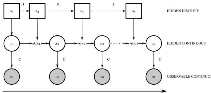
where stis a 1 ⇥ S unit vector that indicates the index of stin the set S. The state transition matrix ⇧, whose elements are ⇧(a, b) = P (st+1 = sa|st = sb), represents the probability of st+1 = sa, given that st = sb. Figure 2.9 is a graphical representation of the evolution of a SLDS in (2.4) and (2.5).
The SLDS approach develops the stochastic algorithms for learning the parameters of the models (2.4) and (2.5) (specially A(sa), Q(sa), ⇧) and estimating st, xt from the observed measurements in a time-series, combining two well known probabilistic approaches: LDS (Kalman Filter) and HMM (forward-backward and Viterbi algorithms). The complexity of
y1 t OBSERVABLE CONTINUOUS ⇧ s1 s2 HIDDEN DISCRETE A(s1) x1 x2 HIDDEN CONTINUOUS C y2 s2 A(s2) x2 y3 s3 A(s3) x3 yt st A(st) xt ⇧ ⇧ C C C
Figure 2.9: Graphical representation of a Switching Linear Dynamic System.
the estimation tasks (filtering, smoothing or finding the most likely sequence) in SLDS com-pared to either LDS or HMM lies on the need to estimate two hidden variables, i.e. st, xt, simultaneously.
The evolution of the time-series in each interval [t, t + 1] is tracked with a linear state-space model as in Equation (2.4); i.e the values of A(st+1)and rt+1(st+1)are associated with the value of s 2 S. Tracking a given time-series with SLDS will yield a sequence of symbols stthat best represent the time-series trends.
Working with SLDS models, it is possible to execute the usual tasks involved in state space representations: prediction, filtering, smoothing and finding the most likely sequence of discrete events.
In order to estimate the most likely sequence based on observed time-series, [44] pro-poses an adaptation of the Viterbi algorithm, commonly used in HMM, for the SLDS case. This algorithm relies on a cost function (C) that considers both the tracking error of the lin-ear state-space variable xtin ((2.4)) and the cost of the transitions for the discrete switching variable stin (2.5).
The method that will be presented in Chapter 4 relies mainly in the algorithm proposed by [44] and henceforth, we will refer to this algorithm as SLDS-Viterbi.