1
Assessing and improving management practices when planning packaging waste
collection systems
Abstract
Packaging waste collection systems are responsible to collect, within a geographic area, three types of packaging materials (paper, glass and plastic/metal) that are disposed by the final consumer into special bins. Those systems are often characterized by having a network with multiple depots that act as transfer and sorting stations, and where the vehicle fleet is based. However, each depot is often managed independently and not as a part of a unique system. In this work, four current tactical/operational practices that contribute to the independent management of each depot are analysed. The change of such practices is investigated and their impact assessed on the total collection cost. A solution methodology based on mathematical formulations is developed to plan service areas, vehicle routes and vehicle schedules taken into account new alternative solutions in managing the system as a whole. Such methodology is applied to a real case study of a company responsible for the collection of the packaging waste in 7 municipalities in mainland Portugal. New service areas, collection routes and vehicle schedules are defined and significant savings are obtained in terms of the total distance travelled as well as in terms of the number of vehicles required, resulting in a decreasing of the total system cost.
Keywords: Collection routes, Service areas, Routes scheduling, Recycling, Waste Management,
Vehicle Routing
1. Introduction
Recycling of packaging materials was imposed by the European Union (EU) to the Members States through the European Community Directive 94/62/EC, which has set targets for recovery and recycling of packaging waste. To meet those targets, a large investment in waste management was made in Portugal since until then all the produced waste was dumped without any kind of treatment. A new collection system - the selective collection – had to be developed given that the traditional routes defined for undifferentiated waste did not fit the particularities of the recycling materials: different vehicles, different collection rates and different bin locations.
The Green Dot System was created in 1996 to promote selective collection, sorting, recovery and recycling of packaging waste in Portugal in order to accomplish the targets set by EU. This system is funded by packers/manufactures who are responsible for products final disposal (according to the Extended Producer Responsibility principle) and had transferred such responsibility to an entity duly licensed for this activity (the Sociedade Ponto Verde (SPV) which manages the Green Dot System). The packers pay a “green dot fee” for each package sent to the market according to its weight and materials used. With the revenues from the green dot fees, SPV supports the selective collection and sorting costs. The selective collection and sorting operations are performed by municipal and multi-municipal waste collection
companies that are paid according to the weight and type of material delivered to SPV. This financial support value, predetermined by the latter, intends to cover only the costs incurred with collection and sorting operations for the packaging waste materials, deducting the costs avoided with undifferentiated collection and landfill disposal. Therefore, it is crucial that waste collection companies operate their collection and sorting systems in an efficient way, otherwise excessive costs are incurred that won´t be refunded. To get more insights on the Green Dot System and on the efficiency of the waste collection companies, please see Marques et al. (2012).
To increase efficiency in the recyclable waste collection systems, an optimized solution in terms of service areas, vehicle routes and vehicle schedules should be pursuit in order to minimize the total collection cost. In packaging waste collection systems operating in Portugal, collection costs represent about 66% to 69%, while sorting costs represent about 11% to 30% of the total costs (APA, 2008). Thus, savings in the collection costs are of great impact on the total costs.
The aim of this work is to build new solutions so as to reduce the collection costs by optimizing the service areas, vehicle routes and vehicle schedules under alternative network management scenarios. The majority of the recyclable collection systems have more than one depot in the network and it is a current practice to manage each depot independently. Therefore, service areas are defined by depot, vehicles are fixed to a depot and only closed routes are allowed (routes starting and ending at the same depot). This work intends to assess and improve four management practices, commonly used by the packaging waste collection systems operating in Portugal, that involve the following assumptions: 1) respect the municipalities boundaries to define service areas; 2) the service areas are defined by depot; 3) the vehicles are fixed to a depot and can only perform routes starting and ending at that depot; and 4) only closed routes are allowed. To achieve this goal the next questions are raised and consequently analysed: if the systems responsible for the collection and sorting of packaging waste are multi-municipal, why should the geographic boundaries of the municipalities define the service area of each depot? If multiple materials are collected in independent routes, why not having service areas by recyclable material? If the system has multiple depots and all vehicles belong to the company, why not sharing the resources (vehicles) among depots? If the system has multiple depots, why not allow routes to start at a depot and to end at a different one? The main contribution of the current work is then on assessing the impact of breaking up with the current tactical/operational practices that consider that depots are managed independently and not in an integrated way. For that we proposed a unified solution methodology that is capable to plan the collection systems exploring more efficient practices. The solution methodology is applied to a real packaging waste collection system and the results are compared with the current solution where the four practices are used.
The remainder of the paper is structured as follows. Section 2 briefly reviews the literature on routing problems. Section 3 describes the main features of the case study. In Section 4 the solution methodology is described and the results of the application to the case study are presented at Section 5. Finally, Section 6 concludes the paper and draws some future research directions.
3
2. Literature Review
Recycling has several environmental and economic benefits such as mitigating resource scarcity, decreasing demand for landfill space and involving savings in energy consumption (Craighill and Powell, 1996). However, the activity of recyclable waste collecting has also several environmental and economic costs since it is basically a transportation activity. To diminish such costs, collection routes should be defined in order to minimize the total distance travelled or the total routing cost. The problem of defining the optimal collection routes is known in the literature as the Vehicle Routing Problem (VRP). This problem is widely studied and several methods were proposed to solve it in the last decades (see the recent surveys of Golden et al. (2008) and Laporte (2009)). However, the routing problem that appears in the packaging waste collection systems goes far beyond the classical VRP. The vehicle fleet is based at multiple depots, multiple products have to be collected and different collection frequencies are observed for each product and site. Therefore, the routing problem arising in the packaging waste collection systems is the Multi-Product, Multi-Depot Periodic Vehicle Routing Problem (MP-MDPVRP), where it has to be decided from which depot the multiple products at each site should be collected, in which day of the planning horizon each site should be visited and what should be the collection visit sequence in order to minimize the total routing cost. Parthanadee and Logendran (2006) presented a mathematical model for the MP-MDPVRP and three tabu search heuristics are developed to solve it. However, the authors had called the problem “multi-product” since several products have to be delivered to customers, but the same customer can be visited by vehicles from different depots. In our case, “multi-product” refers to the fact that the three packaging materials in each site have to be collected from the same depot.
Considering only one product, the MDPVRP has been studied by Hadjiconstantinou and Baldacci (1998) and recently by Vidal et al. (2012). In the former work a heuristic approach based on tabu search has been developed. The heuristic algorithm is applied to a real case of a utility company that provides preventive maintenance services to a set of customers. This company has 17 vehicles, based on 9 depots, to serve 162 customers with a frequency that can vary from once a day to once every four weeks. The large scale problem motivated the authors to apply a heuristic algorithm instead of an exact one. In the latter work, the authors proposed a hybrid genetic algorithm with adaptive diversity control to solve several classes of multi-depot and periodic vehicle routing problems, including the MDPVRP, and applied it to several test instances.
Considering only one depot, several heuristics approaches have been developed for the PVRP where a planning horizon of several days is considered since customers have different visiting frequencies. Beltrami and Bodin (1974), Russel and Igo (1979) and Teixeira et al. (2004) developed heuristic algorithms for the PVRP which were applied to waste collection problems. Mourgaya and Vanderbeck (2007) presented a column generation procedure followed by a rounding heuristic to solve a PVRP with two objectives: minimizing total distance travelled and balance workload among vehicles. Other heuristic applications to PVRP can be found in Christofides and Beasley (1984), Gaudioso and Paletta (1992), Chao et al. (1995), Cordeau et al. (1997) or Alonso et al. (2008), to name a few.
4 Considering a single time unit planning horizon with multiple depots, several works have been published to tackle the MDVRP. Golden et al. (1977), Salhi and Sari (1997), Cordeau et al. (1997), Thangiah and Salhi (2001), Lim and Wang (2005), Lau et al. (2010) are some works where heuristics and meta-heuristics approaches were developed. Laporte et al. (1984; 1988) and Baldacci and Mingozzi (2009) have proposed exact methods to solve the MDVRP. Among the works on multi-depot problems, we highlight one where inter-depot routes are considered. Crevier et al. (2007) study an extension of the MDVRP in which vehicles may be replenished at intermediate depots along their route (Multi-Depot Vehicle Routing Problem with Inter-Depots Routes). The authors propose a heuristic combining the adaptative memory principle and a tabu search method for the generation of a set of routes, and an integer programming model in the execution of a set partitioning algorithm for the determination of the least cost feasible rotations (the authors define rotation as the set of routes assigned to a vehicle).
In waste collection problems there is another critical aspect to address: the estimation of the waste amount to collect at each bin. The majority of works uses deterministic input data. However, recent works like Johansson (2006), Faccio et al. (2011) and Anghinolfi et al. (2013) have approached dynamic routing in waste collection problems, where modern traceability devices, like volumetric sensors, identification RFID (Radio Frequency Identification) systems, GPRS (General Packet Radio Service) and GPS (Global Positioning System) technology, permit to obtain data in real time, which is fundamental to implement an efficient routing plan. The basic idea is that, if the real time position and replenishment level of each vehicle are known, as well as the real time waste level at each bin and which bins have been visited, it is possible to decide which bins should be emptied and which can be avoided at a certain time. This allows an optimization of the route plan and to minimize covered distance and number of vehicles needed, which, as a consequence, would minimize travel time, number of load– unload stops, exhaust emissions, noise and traffic congestion (Faccio et al., 2011).
3. Case Study - a real packaging waste collection system
In Portugal there are 31 recyclable collection systems (SPV, 2011), each one responsible for a certain number of municipalities (Portugal has a total of 308 municipalities). Our case study focuses on the company responsible for the recyclable collection system covering seven rural municipalities with a total area of 6400 km2. This company operates five depots where the collection vehicles are based. One of the depots operates also as a sorting station (depot 235, see Figure 1). The remaining four are only transfer stations where the packaging waste is consolidated and afterwards transferred to the sorting station. Given such logistics network configuration, two types of transportation flows need to be considered, namely, the inbound flow from the collection sites to the depots and the outbound flow from the depots to the sorting station. The collection is performed by a vehicle fleet with no compartments, so each packaging material has to be collected in separated routes. There are 651 Glass bins, 513 Paper bins and 458 Plastic/Metal bins spread over 230 localities (see Figure 1). It is assumed that a collection site corresponds to a locality instead of an individual container in order to reduce the problem size. Due to the proximity of the containers within a locality (an average distance of 650 meters is observed) it is practicable to treat the containers to collect within a
5 locality as a single node. Therefore, a collection site aggregates one or more containers of one or more recyclable materials, meaning that the distance travelled and the time spent within a collection site have to be considered.
All the collection routes start at a depot, visit several localities collecting a single type of material, and return to a depot to unload. Collection is performed five-days a week, eight hours per day, during daytime. It is assumed that the collection sites can be collected at any time of the day within the working period, i.e., between 10 a.m. to 19 p.m. (with a lunch break of an hour). For each site no time windows are considered.
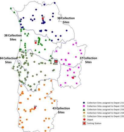
The three recyclable materials have different collection frequencies. Glass has to be collected once a month, Plastic/Metal every two weeks and Paper every week. Therefore, each route has to be scheduled in a four-week planning horizon that is to be repeated every four weeks. Due to vehicle volume capacity constraints and taking into account each material’s density, vehicles can load a maximum of 4500 kg of Glass, 3400 kg of Paper and 600 kg of Plastic/Metal. For the outbound transportation, i.e., from the depots to the sorting station, larger vehicles are used where weight capacities are increased to 12000 kg for Glass, 4000 kg for Paper and 2000 kg for Plastic/Metal. Furthermore, one of the company policies is that each depot is responsible for a fixed set of containers, thus there is a need of defining the depots service areas. Nowadays, the company operates service areas considering the municipalities’ boundaries. Moreover, all recyclable materials at each collection site have to be collected from the same depot, meaning that each depot has only one service area common to all recyclable materials. The current service areas are depicted in Figure 1, which together with the current vehicle routing plan imply an average of 28000 km driven per month (four weeks) and a vehicle fleet of 9 vehicles.
Figure 1. Depot’s location and current service areas
231 233 235 232 234 38 Collection Sites 27 Collection Sites 84 Collection Sites 38 Collection Sites 43 Collection Sites
Collection Sites assigned to Depot 231 Collection Sites assigned to Depot 232 Collection Sites assigned to Depot 233 Collection Sites assigned to Depot 234 Collection Sites assigned to Depot 235 Depot
Given the current solution’s cost, the company envisages the restructure of their service areas and vehicle routes plan in order to decrease such value. An optimized plan is pursued where service areas, vehicle routes and route scheduling can be redefined in a breakthrough scenario, i.e., where service areas do not have to respect municipalities boundaries, can be defined by packaging material, resources can be shared among the depots and open routes between depots are allowed.
4. Solution Methodology
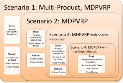
Accordingly to the four practices used by the packaging waste collection systems operating in mainland Portugal, four scenarios will be study wherein each practice is broken cumulatively until the breakthrough scenario is reached (see Figure 2). The first scenario breaks with the practice “respect municipalities boundaries” and maintains the remaining three. In this case, the problem to be solved is the Multi-Product, Multi-Depot Periodic Vehicle Routing Problem (MP-MDPVRP). The second scenario breaks with two practices, “respect municipalities boundaries” and “service areas by depot”, and maintains the remaining two. In this case each packaging material is solved independently. Therefore, a Multi-Depot Periodic Vehicle Routing Problem (MDPVRP) for each packaging material has to be solved. The third scenario breaks with an additional practice, “vehicles are fixed to a depot” while maintaining the “closed routes” practice. Here a MDPVRP with Shared Resources is solved, where the vehicle based at one depot can perform collection routes starting and ending at a different depot. In this scenario, only one relocation movement is allowed per vehicle, i.e., a vehicle based at depot i can travel to depot j to perform closed routes from depot j and then returns to home depot i. It is not allowed two or more relocation movements, such as: a vehicle based at depot i travelling to depot j and then to depot h and returning to depot i. Finally, in the fourth scenario, the breakthrough scenario, the four practices are broken and a MDPRVP with Inter-Depot Routes is solved. At this point open routes between depots are allowed but, at the end of a working day, the vehicles have to return to their home depot.
Figure 2. Scenario’s description
To solve the above scenarios we proposed a solution methodology to define service areas, vehicle routes and schedules. This approach involves four main modules, as it is shown in Figure 3. The first module defines service areas by recyclable material, the second module
Scenario 1: Multi-Product, MDPVRP
Break - Respect Municipalities Boundaries Mantain - Service Areas by Depot - Fixed Vehicles - Closed RoutesScenario 2: MDPVRP
Break - Respect Municipalities Boundaries - Service Areas by Depot Maintain - Fixed Vehicles - Closed RoutesScenario 3: MDPVRP with Shared Resources Break - Respect Municipalities Boundaries - Service Areas by Depot - Fixed Vehicles Break - Respect Municipalities Boundaries - Service Areas by Depot
- Fixed Vehicles - Closed Routes Maintain - Closed Routes Scenario 4: MDPVRP with Inter-Depot Routes
7 defines service areas by depot, the third module defines the final collection routes and the fourth module defines vehicle schedules according to the characteristics of each scenario. This solution methodology is an extension of the method proposed in Ramos et al. (2013b) where only service areas and vehicle routes are defined for the MP-MDVRP. The periodic issue (routes scheduling), shared resources and open routes are not tackled in the mentioned work.
Figure 3. Solution methodology main modules
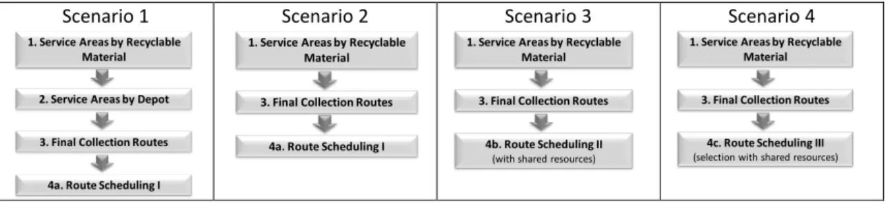
For scenario 1, where a MP-MDPVRP is solved, modules 1, 2, 3 define the service areas and the final vehicle routes for each depot and module 4a schedules, within the planning horizon, the routes generated by module 3 (see Figure 4). For scenario 2, where a MDPVRP is solved, module 1 defines the service areas for each packaging material, module 3 defines the final collection routes and module 4a schedules the routes. For scenarios 3 and 4, only the scheduling module differs from scenario 2. At scenario 3, the scheduling module (module 4b) takes into account that the vehicles can be shared among depots. At scenario 4, besides taking into account a shared-resources solution, the scheduling module (module 4c) considers also all the vehicle routes defined along the solution procedure (open and closed routes defined by module 1) together with the vehicle routes defined at module 3.
Scenario 1 Scenario 2 Scenario 3 Scenario 4
Figure 4. Solution methodology for each scenario
Each module of the solution methodology involves mathematical formulations. Each module will be detailed in the following section.
4.1 Modules description
4.1.1 Module 1: Service Areas by Recyclable Material
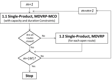
To define service areas by recyclable material, a MDVRP has to be solved for each material. Since mathematical programming solvers cannot solve large size instances of the MDVRP, we adopted the solution method developed in the work of Ramos et al. (2013b) as shown in Figure 5. Notice that m represents the packaging materials, and |M| the total number of materials to be collected.
1. Service Areas by Recyclable Material
2. Service Areas by Depot
3. Final Collection Routes
4. Route Scheduling
4a. Route Scheduling I 4b. Route Scheduling II 4c. Route Scheduling III
1. Service Areas by Recyclable Material
2. Service Areas by Depot
3. Final Collection Routes
4a. Route Scheduling I
1. Service Areas by Recyclable Material
3. Final Collection Routes
4a. Route Scheduling I
1. Service Areas by Recyclable Material
3. Final Collection Routes
4b. Route Scheduling II (with shared resources)
1. Service Areas by Recyclable Material
3. Final Collection Routes
4c. Route Scheduling III
Figure 5. Solution method to solve the MDVRP
Firstly, it is solved a Single-Product, MDVRP with Mixed Closed and Open Routes. This problem involves the definition of the optimal routes to collect one single product, considering a network with multiple depots and allows closed and open routes between depots. As input data, this module requires the distance between each node (collection sites and depots), the weight to be collected and the service time at each collection site (considering only one recyclable material), the vehicle capacity and the maximum time allowed for a working day. The output will be a set of collection routes, where some routes start and end at the same depot (closed routes) while others start and end at different depots (open routes). Since this formulation allows closed and open routes between depots, it should be guarantee that the number of vehicle routes starting and ending at each depot is the same. Note that the number of vehicle routes is not constrained since the vehicle fleet size is one of the model’s outputs. For further details see Ramos et al. (2013a).
If open routes are produced, a MDVRP is solved to close them so that service areas are defined. An open route links two different depots, meaning that collection sites within such route are assigned to two depots instead of just one. By solving a MDVRP to the collection sites that integrate each open route, closed routes are obtained.
Considering the packaging material set M , this solution method have to be run for all materials included in set M .
4.1.2 Module 2: Service Areas by Depot
If service areas by depot are required, module 2 is executed (this will only be of use in scenario 1). Service areas by depot imply that all packaging materials at each collection site are collected from the same depot. Comparing the service areas defined for each packaging material in the previous module, some sites may not respect that rule. Such sites are named as “unclear sites” since there is no agreement among the packaging materials concerning their depot assignment. For those sites, a Multi-Product, MDVRP is solved, where a constraint ensures that all materials at each collection site are allocated to the same depot. This formulation is detailed in Ramos et al. (2013b).
m=1
1.1 Single-Product, MDVRP-MCO
(with capacity and duration Constraints)
Are all routes closed?
1.2 Single-Product, MDVRP
(for each open route)
m=|M|? Stop No Yes m=m+1 Yes No
9 The mathematical formulation for the Multi-Product, MDVRP is only capable of solving small instances, i.e., problems with a small number of unclear sites (lower than 30 unclear sites, according to preliminary tests). Therefore, one way to reduce the problem size is to consider the number of unclear sites between each pair of depot rather than considering all unclear sites at once. For example, a site is “unclear” if it is collected from depot 1 for material Glass and from depot 2 for materials Paper and Plastic/Metal. Therefore, this site is unclear between depots 1 and 2. Since this lack of “clearance” concerns at least two depots, such partition of the unclear sites set would be a natural way to do so. If, with such decomposition, the number of unclear sites for each pair of depots is still above 30, a heuristic assignment rule has to be defined. In this case, the unclear sites are placed according to the assignment made by the material with the highest collection frequency. Some effectiveness tests performed in the work of Ramos et al. (2013b) support such heuristic rule.
4.1.3 Module 3: Final Collection Routes
After defining the service areas (by depot or by recyclable material), module 3 is executed to set the final vehicle routes for each depot and each packaging material. Along with modules 1 and 2 vehicle routes are defined, but the aim of those modules is to establish service areas through the definition of the vehicle routes. Therefore, the defined routes can be improved once the final service areas are set, and this is what module 3 is designed for. The CVRP formulation proposed by Baldacci et al. (2004) is extended to deal with duration constraints. 4.1.4 Module 4: Route Scheduling
Finally, the scheduling module defines for each day of the planning horizon which route should be performed, ensuring that the collection frequency over the planning horizon is fulfilled and a minimum and a maximum time interval between consecutive collections is observed in order to prevent containers overflow. Moreover, it is desirable that the same route is performed by the same vehicle/driver.
Each route k K (defined in the previous module) is characterized by (1) distance dk; (2)
duration bk, which includes travel, service and unloading times; and (3) load Lk. Km is the
routes subset for material m. The collection sites that belong to route k are given by a binary parameter ik that equals 1 if collection site i Vc belongs to route k; and 0 otherwise (Vc is
the nodes set of collection sites). The starting and ending depots for route k are also given by binary parameters Ski and Eki, respectively: Ski equals 1 if route k starts at depot i Vd
while Eki equals 1 if route k ends at depot i Vd (Vd is the node set for depots).
The vehicles are fixed at the depots. Let G be vehicle set. If vehicle g belongs to depot i, the binary parameter gi equals to 1; and 0 otherwise.
The collection frequency of each collection site i with recyclable material m is given by fim
representing how often a collection site has to be visited in the planning horizon. The minimum and maximum interval between two consecutive collections for packaging material
The scheduling model has a single decision variable, which is the binary variable xktg that equals 1 if route k is performed on day t by vehicle g and equals 0 otherwise.
The scheduling module involves three variants: module 4a, where the routes defined at module 3 are scheduled and the vehicle are fixed at each depot; module 4b, where the routes defined at module 3 are scheduled, but the vehicles can be shared among depots; and module 4c, where the vehicles can be shared but the set of routes to be scheduled includes also the routes defined along module 1, where open routes were defined. For module 4a, the objective function is given by Equation (1), while for modules 4b and 4c the objective function is given by Equation (2). s d m V j iV m Mk K t Tg G ij m k ktg ki K k t Tg G ktg kx E x L P d d Min / 2 (1) 1 10 , 1 2 2 / 2 / gi kj ki d s d m gj s d m G g S EK k tTijV ij ktg V j iV mMk K tTgG ij m k ktg ki ki V j iV mMk K tTgG ij m k ktg ki K k tTg G ktg k d x d P L x E S d P L x E x d Min (2)
Equation (1) considers the distance to be travelled (inbound and outbound distance) when vehicles are fixed at depots and cannot be shared among them. The outbound distance considers the number of round-trips between the sorting station and the depots to transfer the entire load collected by the depots (Vsis the sorting stations set). To compute the number
of round-trips needed it is considered the total load collected by a depot and the vehicle capacity for outbound transportation for each material m (Pm). Note that the number of
round-trips is not round upward due to the finitude of the modeled planning horizon. In fact, in the real management of this system round-trips are repeated in all time periods.
Equation (2) considers that although each vehicle belongs to a depot, vehicles can be shared, meaning that they can perform routes assigned to another depot. In this case, two adjustments in the objective function need to be done: (i) add the distance to be travelled between depots when a vehicle belonging to depot i is performing a route of depot j (this is reflected by the fourth term of Equation (2)); (ii) decrease the distance related to the outbound transportation when a vehicle belonging to the sorting station performs routes assigned to a different depot. In this case, the load collected will now be unloaded at the sorting station and not at the transfer depot, so the corresponding outbound distance should not be accounted in the objective function (this is reflected in the third term of Equation (2)). Some constraints are then to be considered in the scheduling models:
m V i f x im c K k t T gG ik ktg m , (3)
Constraint (3) ensures that a collection site i with material m has to be collected fim times over
11 1 : , , 2 0 1 gi d E S K k i jV j ij ktg K k k ktgb x v H t g i V x ki kj d (4)
Constraint (4) states that the total route duration performed by vehicle g on day t will not exceed the maximum number of working hours per day (H). If a vehicle g, belonging to depot i, performs a route starting at depot j, the travel time between i and j (vij) is accounted. It is
assumed that the sites can be collected any time during the working day, i.e., no time windows are being considered concerning the collection site.
m m c G g ik G g g kt ik ktg x i V k K m t t T t t t t I x ' 1 , , , , ' : ,' ' (5)
Constraint (5) states that the same route for material m has to be performed with a minimum time interval of Im. If the collection of site i occurs at day t’, the next collection cannot occur at
the next t days, being t ≤ t’+ Im.
m m m m c G g ik G g g kt ik ktg x i V k K m tt T t t t t A t t A I x ' 1 , , , , ' : ,' ' , ' (6)
Constraint (6) assures the maximum interval Am between consecutive collections. If the
collection of site i occurs at day t’, the next collection cannot occur after t days, being t > t’+Am
and t ≤ t’+ Am +Im. Since the same collection site i has to be collected fim times in the planning
horizon, t have to be limited to t ≤ t’+ Am +Im.
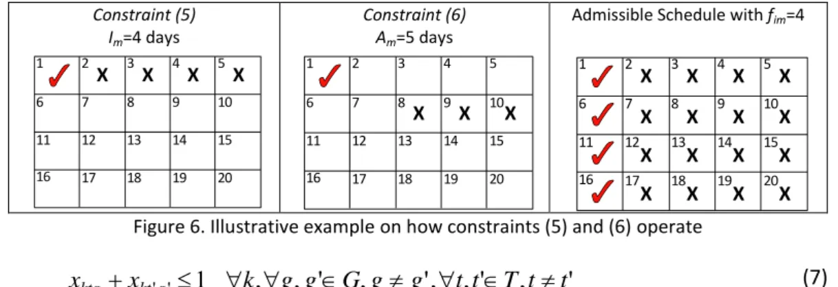
Figure 6 shows an illustrative example on how constraints (5) and (6) are implemented. Considering an Im=4 days and Am=5 days, constraint (5) ensure that if site i is collected at day 1,
it cannot be collected at days 2, 3, 4 and 5. Constraint (6) ensures that if site i is collected at day 1, it cannot be collected at days 8, 9 and 10. If site i has to be collected four times in the planning horizon (fim =4), then one possible schedule is presented at Figure 6.
Constraint (5) Im=4 days
Constraint (6) Am=5 days
Admissible Schedule with fim=4
Figure 6. Illustrative example on how constraints (5) and (6) operate
'
,
'
,
,'
,
'
,
,
1
' 'k
g
g
G
g
g
t
t
T
t
t
x
x
ktg ktg (7)Constraint (7) ensures that the same route has to be performed by the same vehicle along the planning horizon. Therefore, the collection sites are always visited by the same vehicle and driver. G g T t K k xktg {0,1} , , (8)
Variables domain is given in constraint (8).
11 12 13 14 15 6 7 8 9 10 16 17 18 19 20 1 2 3 4 5 X X X X 11 12 13 14 15 6 7 8 9 10 16 17 18 19 20 1 2 3 4 5 X X X 11 12 13 14 15 6 7 8 9 10 16 17 18 19 20 1 2 3 4 5 X X X X X X X X X X X X X X X X
Constraints (3) to (8) are applied in modules 4a and 4b. For module 4c, Constraints (9) to (11) are needed because there are alternative routes to be selected, given that all routes defined along the solution procedure are considered in the scheduling module.
j i V j i t g x x d E S K k E S K k tg k ktg kj ki o i k j k o , , , , 1 1 1 1 ' ' ' ' (9)
Constraint (9) guarantees that all vehicles return to their home depot in case of open routes are selected as part of the solution (Ko is the subset of open routes). If an open route k starting at depot i and ending at depot j is part of the solution, one open route k’ starting at depot j and ending at depot i has also to be part of the solution.
m m c G g ik G g g t k ik ktg x i V k k K m tt T t t t t I x '' ' 1 , , ' , , , ' , ,' ' (10)
In case of module 4c, the consecutive collections can be performed by the same route or by two different routes. Constraint (10) ensures the minimum time interval in case two different routes are collecting the same site i, at consecutive collections.
m m m m c G g ik G g g t k ik ktg x i V k k K m tt T t t t t A t t A I x '' ' 1 , , ' , , , ' , ,' ' , ' (11)
Constraint (11) guarantees the maximum interval Am between consecutive collections when
two different routes collect the same site i.
The output of the scheduling modules is a schedule for each vehicle establishing the routes to be performed in each day.
5. Results analysis
The solution methodology proposed is applied to the packaging waste collection system described at section 3 in order to plan new service areas, new collection routes and new vehicle schedules, while assessing, regarding the total collection cost, the impact of breaking up with the current practices.
The mathematical formulations developed are implemented in GAMS 23.7 and solved through the CPLEX Optimizer 12.3.0, on an Intel Xeon CPU X5680 @ 3.33GHz.
The results for each scenario will be shown, followed up by a cost-analysis considering the distance travelled and the number of vehicles required, assessing the impact of each current practice.
5.1 Scenarios results
5.1.1 Scenario 1: Municipalities’ Boundaries
The first module is run for each one of the three packaging materials: Glass, Paper and Plastic/Metal. The results for formulation 1.1 are shown at
13
Table 1. Results for formulation 1.1
Packaging Material Total Distance No. Closed Routes No. Open Routes Total No. Routes
Glass 3381 km 18 13 31
Paper 11595 km 21 0 21
Plastic/Metal 8047 km 38 11 49
Total 23023 km 77 24 101
The difference in the total distance travelled among the three materials is explained by the collection frequency of each material in the planning horizon. Glass has to be collected once, while Plastic/Metal twice and Paper has to be collected four times. On the other hand, Plastic/Metal is the material with the lowest density among the materials, and thus the vehicle weight capacity for such material is smaller for the same vehicle volume capacity. Therefore, more routes are required, and consequently, more distance is travelled.
Regarding Paper only closed routes are proposed in the final solution, thus there is no need to solve the MDVRP (formulation 1.2). This can be explained by the fact that there is a little difference between the inbound and outbound vehicle’s capacity for Paper. Paper has the smallest increase in vehicle capacity for the outbound capacity (an increase of about 17% - 4000 kg vs. 3400 kg – against an increase of 166% for Glass and 233% for Plastic/Metal) what favors the assignment of more sites to the sorting station to avoid the outbound transportation (as it will imply a greater distance to be travelled as the vehicle capacity is small). For those sites assigned to the sorting station (about 70% of all sites), closed routes are defined in order to avoid the outbound transportation. For the remaining sites, if open routes were defined, the increase in the outbound transportation would not be compensated by the decrease of the inbound transportation by defining open routes.
For the remaining two materials, the open routes are to be redefined into closed ones by formulation 1.2 in Figure 5. As final result, Glass has 17 routes, Paper 21 and Plastic/Metal 12 routes, all closed ones.
The service areas produced for the three materials are shown in Figure 7.
Glass Paper Plastic/Metal
231 233 235 232 234 13 Collection Sites 7 Collection Sites 149 Collection Sites 39 Collection Sites 12 Collection Sites 231 233 235 232 234 16 Collection Sites 0 Collection Sites 122 Collection Sites 39 Collection Sites 3 Collection Sites 231 233 235 232 234 15 Collection Sites 18 Collection Sites 50 Collection Sites 68 Collection Sites 31 Collection Sites
Figure 7. Service areas obtained for each packaging material (Ramos et al., 2013b)
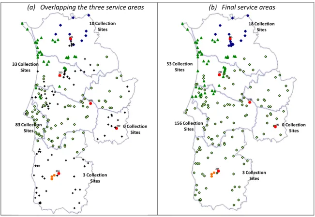
Since different service areas are defined, and Scenario 1 requires equal service areas among the three materials, module 2 is run for the unclear sites. When the three service areas are overlapped, the unclear sites are highlighted (see Figure 8 (a)). 101 unclear sites are identified: 8 sites are unclear between depot 231 and depot 233, 20 sites between depots 232 and 235, 28 sites between depots 234 and 235 and the remaining 45 sites are unclear between depots 233 and 235. The Multi-Product, MDVRP formulation was able to solve the sub-problems with 8, 20 and 28 unclear sites. However, the sub-problem with 45 unclear sites has to be solved by the heuristic rule. The final service areas for Scenario 1 are built as shown in Figure 8 (b).
(a) Overlapping the three service areas (b) Final service areas
Figure 8. (a) Service areas overlapped and (b) final service areas
Having the service areas defined, module 3 is applied to establish the final collection routes for each depot and each packaging material. As a result, one obtains 32 routes to collect Glass, 21 to collect Paper and 49 to collect Plastic/Metal. The total distance travelled in the planning horizon is 24405 km (see Ramos et al. (2013b) for the computational results).
Module 4 is then applied to schedule the 102 collection routes. It is assumed a minimal time interval (Im) to collect Paper of 4 days, for Plastic/Metal 9 days and for Glass 20 days, and a
maximum interval (Am) of 5, 10 and 20 days, respectively. Given the service areas obtained and
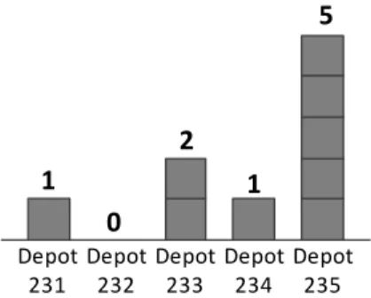
considering that vehicles are fixed at depots, 9 vehicles are required, with the following distribution by depot (Figure 9).
231 233 235 232 234 10 Collection Sites 0 Collection Sites 83 Collection Sites 33 Collection Sites 3 Collection Sites 231 233 235 232 234 18 Collection Sites 0 Collection Sites 156 Collection Sites 53 Collection Sites 3 Collection Sites
15
Figure 9. Vehicle fleet distribution among depots in scenario 1
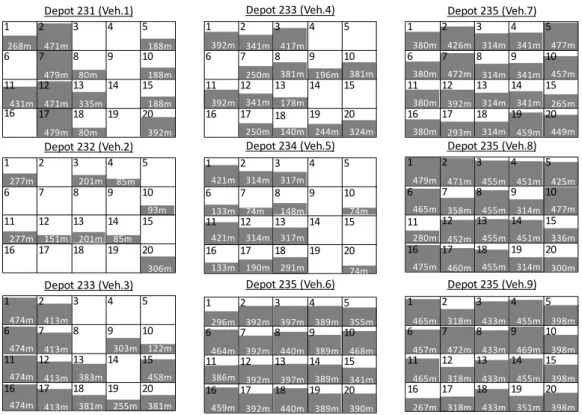
The nine vehicle schedules are shown in Figure 10, where the usage time (in minutes) is identified for each day of the planning horizon. It can be seen that vehicle 4, based at depot 234, has the lowest usage rate since this depot is responsible to collect only three collection sites (see Figure 8 (b)). Two vehicles are assigned to depot 233: vehicle 2 operates 3950 minutes per month, with a usage rate of 41% (3950 minutes/(20 days x 480 minutes)); while vehicle 3 operates 5632 minutes, with a usage rate of 59%. Given the sum of the usage rates, a macro analysis could conclude that the workload of depot 233 requires only one vehicle. However, given the routes duration and the maximum duration of a working day, it is not possible to perform all routes with a single vehicle. For depot 235, that is responsible to collect 156 sites, five vehicles are needed. These vehicles are used every day of the planning horizon and the minimum usage rate among them is 74% (vehicle 8) and the maximum is 86% (vehicle 9). Note that Depot 235 act also as the sorting station and, therefore, a larger number of collection sites were assigned to it.
Figure 10. Schedule by vehicle in scenario 1
Depot 231 Depot 232 Depot 233 Depot 234 Depot 235 1 0 2 1 5 1 2 3 4 5 188m 188m 399m 370m 399m 152m 360m 399m 11 12 13 14 15 6 7 8 9 10 370m 188m 399m 16 17 18 19 20 55m 55m 356m 381m Depot 231 (Veh.1) 1 2 3 4 5 355m 361m 370m 479m 152m 171m 11 12 13 14 15 6 7 8 9 10 16 17 18 19 20 55m 140m 349m 280m Depot 233 (Veh.2) 474m 416m 122m 360m 77m 110m Depot 233 (Veh.3) 215m 211m 227m 74m 349m 74m 361m 399m 1 2 3 4 5 110m 399m 474m 6 7 8 9 10 463m 399m 474m 11 12 13 14 15 211m 294m 337m 399m 474m 16 17 18 19 20 122m 211m 1 2 3 4 5 149m 133m 360m 399m 11 12 13 14 15 6 7 8 9 10 370m 16 17 18 19 20 Depot 234 (Veh.4) 476m 294m 370m 375m 163m Depot 235 (Veh.5) Depot 235 (Veh.6) 396m 477m 133m 133m 149m 282m 1 2 3 4 5 6 7 8 9 10 16 17 18 19 20 11 12 13 14 15 375m 377m 396m 391m 434m 396m 163m 360m 375m 386m 383m 375m 396m 344m 468m 263m 370m 448m 315m 419m 439m 1 2 3 4 5 6 7 8 9 10 11 12 13 14 15 413m 452m 419m 444m 315m 439m 456m 314m 472m 452m 444m 461m 406m 326m 338m 314m 370m 435m 403m Depot 235 (Veh.8) Depot 235 (Veh.9) 145m 314m 1 3 4 5 6 8 9 10 11 12 13 14 15 363m 403m 383m 418m 403m 392m 418m 363m 403m 426m 422m 190m 367m 314m 459m 370m 369m 376m 407m 314m 1 3 4 5 6 8 9 10 11 12 13 14 15 472m 476m 407m 433m 478m 407m 433m 314m 471m 467m 433m 341m 407m 433m 16 17 18 19 20 16 18 19 20 Depot 235 (Veh.7) 206m 281m 370m 471m 312m 392m 278m 1 2 3 4 5 6 7 8 9 10 11 12 13 14 15 449m 312m 392m 389m 312m 429m 389m 129m 413m 312m 389m 463m 392m 389m 16 17 18 19 20 2 7 16 17 18 19 20 17 2 7 168m
The results presented by module 4a are optimal ones given the set of routes defined by the previous module. The scheduling model run in 126 seconds and has an optimal value of 24405 km. See Table 2 for the computational results.
Table 2. Computational results for module 4a in scenario 1
Number of Variables Number of Constraints Running Time (seconds) Gap (%) Module 4a 36 541 1 382 831 126 0%
5.1.2 Scenario 2: Service Areas by Recyclable Material
In this scenario, service areas are defined by packaging material and are obtained after module 1, as it is shown in Figure 7. The service areas are quite different between recyclable materials. For instance, depot 234 is responsible to collect 12 sites for material Glass, but only 3 sites for Paper and 31 sites for Plastic/Metal; depot 232 does not have any site assigned where Paper should be collected, while for Glass and Plastic/Metal, a total of 7 and 18 sites are assigned, respectively.
Module 3 is applied to each depot and each packaging material to define the final collection routes. A solution with a total of 23294 km is obtained, where 21 routes are created to collect Paper, 50 to collect Plastic/Metal and 32 to collect Glass. The computational results can be seen at Ramos et al. (2013b).
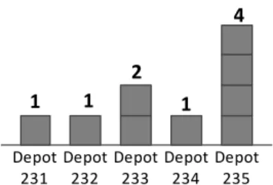
Route scheduling is done by module 4a, where the routes are assigned to a day in the planning horizon and to a vehicle, assuming that sharing resources are not allowed. In this scenario, 9 vehicles are also required, but with a different distribution by depot (see Figure 11).
Figure 11. Vehicle fleet distribution among depots in scenario 2
Scheduling results for each vehicle are shown in Figure 12. Vehicle 1, based at depot 231, has a usage rate of 42%; vehicle 2, based at depot 232, has the lowest usage rate of 18% since it is again the depot with lowest number of collection sites assigned; depot 233 needs two vehicles (vehicle 3 and 4) with a usage rate of 61% and 44%, respectively; vehicle 5, based at depot 234, has a usage rate of 34%; finally, depot 235 has four vehicles, all of them with a high usage rate (83%, 78%, 87% and 85%). Depot 231 Depot 232 Depot 233 Depot 234 Depot 235 1 2 1 4 1
17
Figure 12. Schedule by vehicle in scenario 2
The results presented by module 4a are the optimal ones given the set of routes defined by the previous module. The scheduling model run in 98 seconds and has an optimal value of 23294 km (see Table 3).
Table 3. Computational results for module 4a in scenario 2
Number of Variables Number of Constraints Running Time (seconds) Gap (%) Module 4a 25 921 838 483 98 0%
5.1.3 Scenario 3: Sharing Resources
In this scenario, service areas and vehicle routes are the ones defined for scenario 2. The main difference between scenarios 2 and 3 concerns the scheduling module: vehicles based in one depot can perform closed routes of other depots in scenario 3. In this case, it is expected that the distance travelled will increase since the vehicles have to move between depots, but the number of vehicles will decrease.
We test a solution with eight vehicles, distributed by depot as shown in Figure 13(a), and the total distance travelled increases to 23421 km (more 0.6% comparing with the previous scenario). A solution with seven vehicles was also tested (see Figure 13(b)), and the total distance obtained is now 24198 km (more 3.9% than scenario 2). No integer solution is obtained if only six vehicles are available.
268m 471m 479m 431m 471m 11 12 13 14 15 6 7 8 9 10 335m 479m 16 17 18 19 20 80m 55m 392m Depot 231 (Veh.1) 1 2 3 4 5 277m 370m 277m 11 12 13 14 15 6 7 8 9 10 16 17 18 19 20 306m Depot 232 (Veh.2) 413m 122m 360m 381m 381m Depot 233 (Veh.3) 201m 85m 85m 474m 1 2 4 5 474m 413m 6 7 8 9 10 122m 474m 413m 211m 458m 474m 413m 16 17 18 19 20 303m 383m Depot 233 (Veh.4) Depot 234 (Veh.5) Depot 235 (Veh.6) 190m Depot 235 (Veh.8) Depot 235 (Veh.9) Depot 235 (Veh.7) 1 2 3 4 5 188m 188m 188m 80m 93m 151m 201m 11 12 13 14 15 255m 3 133m 291m 74m 2 3 4 5 421m 314m 360m 399m 12 13 14 15 6 7 8 9 10 370m 16 17 18 19 20 74m 421m 314m 1 317m 133m 148m 74m 11 317m 296m 464m 370m 392m 440m 389m 459m 1 2 3 4 5 6 7 8 9 10 16 17 18 19 20 11 12 13 14 15 392m 397m 389m 355m 440m 389m 468m 386m 392m 397m 341m 392m 389m 390m 380m 380m 370m 472m 314m 341m 380m 1 2 3 4 5 6 7 8 9 10 11 12 13 14 15 426m 314m 341m 477m 314m 341m 457m 380m 392m 314m 265m 293m 459m 449m 16 17 18 19 20 479m 465m 370m 358m 455m 451m 475m 1 2 3 4 5 6 7 8 9 10 11 12 13 14 15 471m 455m 451m 425m 455m 314m 477m 280m 452m 455m 336m 460m 300m 16 17 18 19 20 314m 465m 457m 370m 472m 433m 455m 267m 1 3 4 5 6 8 9 10 12 13 14 15 318m 433m 455m 398m 433m 469m 398m 318m 433m 398m 318m 351m 398m 2 7 16465m17 18 19 20 11 392m 370m 250m 140m 1 3 4 5 6 8 9 10 11 12 13 14 15 341m 381m 196m 381m 392m 341m 178m 250m 244m 324m 16 17 18 19 20 2 7 417m 133m 190m 291m 74m
(a) 8 vehicles (b) 7 vehicles
Figure 13. Vehicle fleet distribution among depots in scenario 3 with (a) 8 and (b) 7 vehicles
The vehicle schedules for the seven-vehicle solution are shown at Figure 14. In this solution five out of the seven vehicles have high usage rates. Vehicle 2, based at depot 233, has the highest rate, 95%. Comparing with the previous scenario, depot 233 has one less vehicle, meaning that a higher usage rate is achieved. The remaining routes from depot 233 are now performed by vehicles based at depot 231 and 235, contributing for a higher usage rate of those vehicles. Vehicles based at depot 235 have usage rates varying from 87% to 91%. Besides performing routes from depot 235, these vehicles execute routes assigned to depot 233, as mentioned, and to depot 232, since in this solution no vehicles have been based in that depot. Vehicle 1, based at depot 231, has a usage rate of 51%, nine percent higher than in the previous scenario, since it also performs routes of depot 233. This is also the case with vehicle 3, based at depot 234, which now increases its usage rate to 37% (34% in the previous scenario) as it performs routes assign to depot 232.
Figure 14. Schedule by vehicle in scenario 3
Figure 15 illustrates the routes performed by vehicle 1, based at depot 231, on days 4 and 14. In those days, vehicle 1 has to travel to depot 233, perform route 104 to collect Plastic/Metal,
Depot 231 Depot 232 Depot 233 Depot 234 Depot 235 1 1 1 4 1 Depot 231 Depot 232 Depot 233 Depot 234 Depot 235 1 1 1 4 0 152m 335m 152m 11 12 13 15 6 7 8 9 399m 163m 479m 55m 456m Depot 231 (Veh.1) Depot 233 (Veh.2) 184m 122m 360m 239m 207m Depot 234 (Veh.3) 323m 1 2 4 5 444m 75m 6 7 8 9 10 350m 133m 211m 310m 222m 75m 16 17 18 19 20 111m 184m Depot 235 (Veh.4) Depot 235 (Veh.5) Depot 235 (Veh.6) Depot 235 (Veh.7) 188m 456m 188m 479m 11 12 13 14 15 111m 3 475m 454m 370m 457m 397m 460m 1 2 3 4 5 6 7 8 9 10 11 12 13 14 15 414m 397m 472m 433m 397m 471m 433m 475m 425m 464m 433m 464m 476m 370m 449m 463m 398m 443m 1 2 3 4 5 6 7 8 9 10 11 12 13 14 15 479m 463m 398m 392m 463m 398m 392m 478m 479m 463m 392m 449m 398m 392m 16 17 18 19 20 355m 472m 370m 468m 380m 465m 446m 1 2 3 4 5 6 7 8 9 10 11 12 13 14 15 477m 380m 452m 336m 470m 461m 306m 469m 477m 380m 300m 468m 358m 16 17 18 19 20 468m 457m 437m 370m 447m 389m 478m 477m 1 3 4 5 6 8 9 10 12 13 14 15 432m 432m 478m 457m 389m 341m 455m 432m 432m 457m 479m 341m 455m 2 7 16458m17 18 19 20 11 399m 1 2 3 4 5 429m 204m 10 14 429m 16 17 18 19 20 458m 478m 370m 463m 474m 413m 478m 1 2 3 4 5 6 7 8 9 10 11 12 13 14 15 469m 477m 413m 474m 474m 413m 474m 383m 473m 477m 474m 463m 413m 474m 16 17 18 19 20 310m 239m 392m 16 17414m18397m19 20433m
19 unload at depot 233, and then return to its home depot. In those days, the vehicle 1 is used during 429 minutes.
Figure 15. Illustration of the routes performed by vehicle 1 on days 4 and 14
In terms of computational results, module 4b has not been able to prove optimality within the time limit of one hour, but a low gap is obtained (see Table 4).
Table 4. Computational results for module 4b in scenario 3 with seven vehicles
Number of Variables Number of Constraints Running Time (seconds) Gap (%) Module 4b 33603 1129857 3600 0.3%
5.1.4 Scenario 4: Open Routes between Depots
Scenario 4 breaks up with all four practices mentioned, meaning that open routes are allowed between depots. In scenario 3, vehicles can be shared among depots but they travel empty between depots. In scenario 4, the main idea is to minimize the number of those empty routes. In order to do so, advantage will be taken from the open routes between depots generated at module 1 which allow the vehicle relocation. Therefore, the relocating movements can now be collection routes and not only empty routes. The scheduling module 4c considers routes generated by modules 1 and 3, which are closed and open routes, and selects the ones that should take part in the final schedules.
The total distance decreases when compared with the previous scenario. With eight vehicles, a total distance of 23181 km is achieved, while a total of 23687 km is obtained if seven vehicles are used.
The each of the seven vehicles schedules are shown at Figure 16. Vehicle 1 is now operating 4077 minutes, corresponding to 42% of usage rate. Vehicle 2 has a usage rate of 92% while vehicle 3 has increased its usage rate to 47% (37% in the previous scenario) since it performs open routes between depots 234, 232 and 235. The four vehicles based at depot 235 maintain high usage rates (from 85% to 91%).
231 233 Days 4 and 14: Routes Duration Direct route 231-233 24 m Route 104 381 m Direct route 233-231 24 m Total 429 m
Figure 16. Schedule by vehicle in scenario 4
Figure 17 shows the routes performed by vehicle 3, based at depot 234, on days 1 and 11 to illustrate the sharing resources allowed by considering open routes. One closed route and two open routes between depot 234 and depot 232 are performed by this vehicle on these days.
Figure 17. Illustration of the routes performed by vehicle 3 on days 1 and 11
Concerning the computational results for module 4c with seven vehicles (see Table 5), one should say that optimality has not been proven within the time limit of one hour, but a low gap is obtained (0.3%).
Table 5. Computational results for module 4c in scenario 4 with seven vehicles
Number of Variables Number of Constraints Run Time (seconds) Gap (%) Module 4b 38041 1241843 3600 0.3% 362m 268m 204m 11 12 13 15 6 7 8 9 399m 268m 399m 55m 268m Depot 231 (Veh.1) Depot 233 (Veh.2) 282m 122m 270m 460m Depot 234 (Veh.3) 281m 458m 281m 211m 392m 184m 16 17 18310m19 20 Depot 235 (Veh.4) Depot 235 (Veh.5) Depot 235 (Veh.6) Depot 235 (Veh.7) 479m 11 12 13 14 15 468m 451m 370m 428m 392m 451m 1 2 3 4 5 6 7 8 9 10 11 12 13 14 15 445m 392m 438m 453m 392m 328m 479m 477m 465m 446m 332m 435m 455m 370m 447m 433m 477m 455m 1 2 3 4 5 6 7 8 9 10 11 12 13 14 15 436m 433m 477m 403m 433m 475m 476m 456m 436m 433m 418m 479m 314m 336m 16 17 18 19 20 389m 389m 370m 457m 380m 398m 389m 1 2 3 4 5 6 7 8 9 10 11 12 13 14 15 439m 380m 398m 441m 380m 398m 391m 389m 465m 380m 399m 422m 476m 16 17 18 19 20 398m 428m 463m 370m 397m 341m 436m 455m 1 3 4 5 6 8 9 10 12 13 14 15 397m 453m 436m 455m 341m 480m 455m 397m 453m 455m 397m 480m 455m 2 7 16463m17 18 19 20 11 399m 1 2 3 4 5 80m 10 14 16 17 18 19 20 467m 381m 370m 455m 413m 474m 498m 1 2 3 4 5 6 7 8 9 10 11 12 13 14 15 446m 461m 474m 398m 413m 474m 461m 361m 449m 413m 473m 455m 474m 461m 16 17 18 19 20 443m 460m 427m 16 17421m18392m19 20480m 188m 340m 188m 163m 72m 102m 310m 1 2 3 5 6 7 8 10 320m 4 9 281m Days 1 and 11: Routes Duration Route 46 74 m Route 43 150 m Route 88 57 m Total 281 m 232 234 #88 #43 #46
21
5.2 Cost Analysis
As mentioned in the previous section, the obtained solutions vary between 23181 km and 24405 km and between 7 to 9 vehicles. Table 6 summarizes the results for the scenarios studied. It shows that scenario 4a is the scenario with the lowest distance travelled per month (23181 km) while scenarios 3b and 4b require the lowest number of vehicles and drivers (7).
Table 6. Results for each scenario
Scenario Distance No. Vehicles No. Drivers
1 24405 km 9 9 2 23294 km 9 9 3a 23421 km 8 8 3b 24198 km 7 7 4a 23181 km 8 8 4b 23687 km 7 7
To compare those solutions a cost-analysis is performed. Three main costs will be computed for each solution: fuel costs, vehicles depreciation costs and driver’s costs. The fuel costs are a linear function of the distance travelled. It has been estimated 0.5€ per kilometer driven. Vehicle depreciation is estimated considering vehicles acquisition cost and the useful life assumed for taxes purpose. In particular, the acquisition cost is about 100000€ and the useful life is of 5 years, which leads to an annual depreciation of 20000€. The drivers costs are estimated in 900€ per month, paid 14 months per year, and it is considered one driver per vehicle.
Figure 18 depicts the total cost for the current solution and for each scenario studied. Scenario 1 has 12.8% less distance travelled than in the current solution and the total annual cost decreases 5% if the municipalities’ boundaries are not respected when defining the service areas. Comparing scenario 2 (service areas are defined by packaging material) to scenario 1 (service areas by depot), the distance travelled decreases 5%, while the required number of vehicles is maintained. The total cost decreases in 1.7% when compared to scenario 1 and 6.4% when compared to the current solution. The largest decrease in the total cost is obtained in the scenario where resources are shared among depots (scenarios 3 and 4). In scenario 3b, the total cost decreases 13.3% regarding scenario 2 and 18.9% when compared to the current solution. These gains come from sharing vehicles among depots which allows the reduction of the number of vehicles to seven. When open routes between depots are allowed, the total distance travelled decreases even more (23687 km against 24198 km, about 2%) and the total cost decreases about 20% when comparing with the current solution.
22
Figure 18. Total cost for each scenario studied
Significant savings are obtained when some of the current practices are removed. However, from an operations management perspective, it is more complex to manage scenario 4, where three different service areas, shared vehicles and open routes have to be dealt with, than the current solution where each depot has one service area, with vehicles assigned and only closed routes, which allows each depot to act independently. However, these latter practices lead to a larger travelled distance and more resources, as vehicles and drivers. In the breakthrough scenario (scenario 4), all depots and vehicles are integrated and act as part of the same system. This kind of solution decreases the distance travelled and the resources needed but demands a decision support system to help managing the increased complexity. The solution methodology developed in this work can be seen as a main pillar towards the development of a decision support system supporting the routes definition and vehicle schedules under an innovative scenario.
6. Conclusions
In this paper four practices currently used by recyclable collection systems operating in Portugal have been analyzed so as to propose improvements on their setups aiming at better a systems operation. Given that the systems in study have multiple depots, but are managed independently, the main idea explored was to manage operations in an integrated way so that gains in terms of efficiency could be achieved, by decreasing the total operational costs. To achieve this goal this paper developed a unified solution methodology that is capable to plan the collection systems exploring more efficient practices. This solution methodology is applied to a real packaging waste collection system. Four scenarios were analysed, developed by cumulatively removing each of the four practices. The problems solved are the Multi-Product, Multi-Depot Periodic Vehicle Routing Problem, the Multi-Depot Periodic Vehicle Routing Problem, the Multi-Depot Periodic Vehicle Routing Problem with Shared Resources and Multi-Depot Periodic Vehicle Routing Problem with Inter-Depot Routes. The solution methodology defines service areas and vehicle routes in an integrated way and afterwards assigns the routes to a day of the planning horizon accordingly to each scenario.
0 50000 100000 150000 200000 250000 300000 350000 400000 450000 500000 Current Solution
Scenario 1 Scenario 2 Scenario 3a Scenario 3b Scenario 4a Scenario 4b Driver Cost Vehicle Cost Fuel Cost 475400€ 452683€ 444811€ 413037€ 385487€ 411477€ 382166€
23 Each scenario was evaluated in terms of travelled distance and number of vehicles required. Also the total annual cost of each scenario considering fuel costs, vehicle depreciation costs and driver’s costs, was calculated. It was concluded that by removing the practice of not sharing resources among depots implies the highest impact on the total cost, since sharing resources enables a decrease up to two vehicles. Also, defining service areas by recyclable material instead of depot (scenario 2 versus scenario 1) lead to a positive impact on the total cost of 1.7%. Sharing resources instead of having the vehicle fixed at the depots (scenario 3 versus scenario 2) conducted to a positive impact of 13.3% (the highest impact, as mentioned), and performing also open routes instead of allowing only closed routes (scenario 4 versus scenario 3) resulted in a positive impact of 0.9% in the total cost. Finally, comparing the current solution with the innovative scenario (scenario 4, where all of the four practices are removed), a decrease of 20% in the total cost was observed.
It is a fact that each scenario studied increased the complexity of managing operations within the recyclable collection systems, but significant costs savings have been attained. Moreover, the current situation is driven by management options cause by political issues that in this case lead to the use of municipal boundaries when planning the systems. Such practice proved to diminish the system’s efficiency and consequently alternative solutions should be pursued. The improved results needed, however, to be demonstrated and discussed with the management. This was achieved, in this work, through a close collaboration between the research and the company management teams.
As future work and still aiming to further improving operation another alternative operational practice can be studied. This is the night collection in opposite to the daytime collection, the latter in use in the packaging collection system in study. Notice, however that performing a daytime collection activity may lead to a decrease in the overall system efficiency given the traffic congestion that may slow down collection. Night collection however can increase the collection efficiency in tradeoff with an increase of personnel costs.
The solution methodology proposed defines firstly the service areas and vehicle routes in an integrated way, and the scheduling decisions are taken in a second phase. This sequential method causes a low usage rate of some vehicles, representing a pitfall of the proposed methodology. A tighter integration of those decisions would lead to higher usage rates, and therefore, better results. As future research, the solution methodology should be improved to tackle simultaneously the three decisions. Also it will be interesting to explore as future work the solution of the current problem by alternative solution techniques as meta-heuristics and compared with the results obtained. Another future work direction is to apply this methodology to other packaging collection systems in order to quantify the results of more case studies so as to corroborate the conclusions of the current work.
Acknowledgement
This work was partially supported by the CMA/FCT/UNL under the project PEst OE/MAT/UI0297/2011.
References
Alonso, F., Alvarez, M.J., Beasley, J.E., 2008. A tabu search algorithm for the periodic vehicle routing problem with multiple vehicle trips and accessibility restrictions. J Oper Res Soc 59, 963-976.
Anghinolfi, D., Paolucci, M., Robba, M., Taramasso, A.C., 2013. A dynamic optimization model for solid waste recycling. Waste Management 33, 287-296.
APA, 2008. Avaliação dos custos dos SMAUTs com as operações de recolha e triagem. url: http://www.tratolixo.pt/Comunicacao/Paginas/equilibrioValoresContra.aspx (acessed on 26/10/2012) Baldacci, R., Mingozzi, A., 2009. A unified exact method for solving different classes of vehicle routing problems. Math Program 120, 347-380.
Beltrami, E.J., Bodin, L.D. 1974. Networks and Vehicle Routing for Municipal Waste Collection, Networks, 4, 65-94.
Chao, I.M., Golden, B.L., Wasil, E., 1995. An Improved Heuristic for the Period Vehicle-Routing Problem. Networks 26, 25-44.
Christofides, N., Beasley, J.E., 1984. The Period Routing Problem. Networks 14, 237-256.
Cordeau, J.F., Gendreau, M., Laporte, G., 1997. A tabu search heuristic for periodic and multi-depot vehicle routing problems. Networks 30, 105-119.
Craighill, A.L., Powell, J.C., 1996. Lifecycle assessment and economic evaluation of recycling: A case study. Resour Conserv Recy 17, 75-96.
Crevier, B., Cordeau, J.F., Laporte, G., 2007. The multi-depot vehicle routing problem with inter-depot routes. Eur J Oper Res 176, 756-773.
Faccio, M., Persona, A., Zanin, G., 2011. Waste collection multi objective model with real time traceability data. Waste Management 31, 2391-2405.
Gaudioso, M., Paletta, G., 1992. A Heuristic for the Periodic Vehicle-Routing Problem. Transp Sci 26, 86-92.
Golden, B.L., Magnanti, T.L., Nguyen, H.Q., 1977. Implementing Vehicle Routing Algorithms. Networks 7, 113-148.
Golden, B., Raghavan, S., Wasil, E. (Eds.). Vehicle Routing Problem: Latest Advances and New Challenges, 2008.
Hadjiconstantinou, E., Baldacci, R., 1998. A multi-depot period vehicle routing problem arising in the utilities sector. J Oper Res Soc 49, 1239-1248.
Johansson, O.M., 2006. The effect of dynamic scheduling and routing in a solid waste management system. Waste Management 26, 875-885.
Laporte, G., 2009. Fifty Years of Vehicle Routing. Transp Sci 43, 408-416.
Laporte, G., Nobert, Y., Arpin, D., 1984. Optimal solutions to capacitated multi-depot vehicle routing problems. Congr Numer 44, 283-292.
Laporte, G., Nobert, Y., Taillefer, S., 1988. Solving a Family of Multi-Depot Vehicle-Routing and Location-Routing Problems. Transp Sci 22, 161-172.
Lau, H.C.W., Chan, T.M., Tsui, W.T., Pang, W.K., 2010. Application of Genetic Algorithms to Solve the Multidepot Vehicle Routing Problem. IEEE Trans Autom Sci Eng 7, 383-392.