© 2004 Museu de Ciències Naturals ISSN: 1578–665X
Lokki, H. & Saurola, P., 2004. Comparing timing and routes of migration based on ring encounters and randomization methods. Animal Biodiversity and Conservation, 27.1: 357–368.
Abstract
Comparing timing and routes of migration based on ring encounters and randomization methods.— A method for comparing two migration routes is introduced. In the method are needed approximations of the average daily positions which are computed based on averages of dates and of positions in a window sliding through the encounters ordered in ascending order by date. The method contains two tests. The first, global, test statistic compares the entire migration routes and is the average of the distances between the daily positions of the two routes to be compared. The second test is used to identify sections during migration where the routes may deviate and is based on consecutive averages of the distances of short time periods between the daily positions of the two routes. A randomization test is used to assess the statistical significance of the test statistics in both components. The methods are applied to artificial and real data. Examples of the use of the method are computed with data sets of ring recoveries of Common terns (Sterna hirundo) and Ospreys (Pandion haliaetus) ringed in Finland in 1930–2002.
Key words: Migration route, Migration timing, Ring encounters, Randomization. Resumen
Estudio comparativo de la adecuación temporal y de las rutas migratorias mediante el empleo de hallazgos de anillas y métodos de randomización.— El trabajo presenta un método para comparar rutas migratorias. El método utiliza aproximaciones para el cálculo de las localizaciones medias diarias basadas en las fechas y localizaciones promedio, en una ventana que se va desplazando a lo largo de las distintas observaciones ordenadas en orden ascendente según fecha. El método incluye dos pruebas estadísticas. La primera compara de forma global todas las rutas migratorias, y lo que se compara es la media de las distancias entre las distintas posiciones diarias de las dos rutas. La segunda prueba permite identificar tramos durante la migración en los que las rutas se pueden desviar, y se basa en promedios consecutivos de las distancias de breves períodos de tiempo entre las posiciones diarias de las dos rutas. Se utiliza una prueba de randomización para evaluar la relevancia estadística de las pruebas en ambos componentes. Los métodos se aplican a datos artificiales y reales. Los ejemplos del empleo del método se calculan con conjuntos de datos de recuperaciones de anillas de charranes comunes (Sterna hirundo) y de águilas pescadoras (Pandion haliaetus) anillados en Finlandia entre 1930 y 2002.
Palabras clave: Ruta migratoria, Adecuación temporal de las migraciones, Hallazgos de anillas, Randomización.
Heikki Lokki, Dept. of Computer Science, P. O. Box 68, FIN–00014 Univ. of Helsinki, Finland.–Pertti Saurola, Finnish Museum of Natural History, P. O. Box 17, FIN–00014 Univ. of Helsinki, Finland.
Corresponding author: H. Lokki. E–mail: [email protected]
Comparing timing and routes of
migration based on ring encounters
and randomization methods
We present the route comparison method and study its performance with artificial and real data. The real data used are recoveries of Common terns (Sterna hirundo) and Ospreys (Pandion haliaetus) ringed in Finland in 1930–2002. The biological interpretations of the findings are not presented in this paper.
M a t e ria l a nd m e t hods
Comparison of two migration routes for geographical or temporal differences
A population of migrants consists of a set of triplets P(t,x(t),y(t)) containing all the locations (x(t),y(t)) of all individual birds of the group. Time t can be restricted to a period of calendar years or whole years can be considered. Here we consider time t as a discrete variable so that each individual is recorded once a day.
The population is divided into two groups, A and B. For each group, the average daily position can be simply computed as with a simi-lar average for group B. Then the distance between the average positions of the two routes at each time is defined as
and finally, the average of the differences is defined as
where m is the number of days in the migration route.
Two populations P(t,x(t),y(t)), summarized in daily positions of migration routes, can differ in two ways: geographically and/or temporally. When two routes differ only geographically the tracks of the routes are different but the timing of migra-tion of the two groups do not differ. When two routes differ only temporally, route points of the groups are at the same location on different dates. The temporal difference or difference in timing of the migration can originate in many ways: the start of the migration of birds of the two groups can occur in different periods of time and/ or the speed of the migration can be different even in different periods during migration. In the s c o p e o f t h i s pa p e r c o m p a r i s o n s o f t w o populations are reasonable only if the starting and ending areas of the migration are the same for both populations.
The encounters along migration routes are often made by the general public and are not sampled systematically. The following assump-tions are necessary: (1) the dates and locaassump-tions of encounters are recorded accurately; (2) en-counters are independent of each other; (3) indi-viduals of both populations are encountered with the same pattern. We expect that the assumption I nt roduc t ion
One of the early goals of bird ringing was to study migration. In this paper we introduce a method for comparing timing and routes of migration based on encounters along birds’ flyways from two groups of birds. The two groups A and B to be compared could be different sexes, different age classes of a species, different causes of recoveries such as "found dead" or "killed", or encounters from different decades.
The difference in timing of migration has been studied by examining differences in peak pas-sages of birds (e.g. Saurola, 1981; Jenni & Kéry, 2003). Fourier analysis has been used in describ-ing migration patterns and plottdescrib-ing the position– date relation (Perdeck, 1977). Perdeck & Clason (1982, 1983) analyzed flyways and sex-based differences in migration and winter quarters of Anatidae ringed in the Netherlands on the basis of average positions of recoveries in disjoint time intervals. Munro & Kimball (1982) used the Mardia–Watson–Wheeler test (Batschelet, 1981) in testing for similarity in ring recovery patterns. It has been shown (Lokki & Saurola, 1987) that the Mardia–Watson–Wheeler test does not per-form well in two–sample location problems and significance can also be caused by unequal variances in the ring recovery patterns to be compared. In addition Munro & Kimball (1982) compared recovery dates of harvested mallards by testing the mean dates of recoveries of ent groups and they found out significant differ-ences between groups in the average arrival time to the areas where the mallards were hunted. The distributions of Common tern (Sterna hirundo) and Arctic tern (Sterna paradisaea) recoveries of birds ringed in Finland have been plotted accord-ing to recovery month and latitude in order to illustrate the temporal patterns of migration (Saurola, 1978). In Swedish Bird Ringing Atlas (Fransson & Petterson, 2001) the differences be-tween mean positions of recoveries of various time periods are tested by a randomization test (Lokki & Saurola, 1987). An extensive overview of many aspects of the study of migration routes has been written by Bairlain (2001).
In the literature cited, the geographical and temporal differences of migration are studied sepa-rately. The geographical difference is often studied using algorithms for two–sample location prob-lems and the temporal component is excluded by restricting the time of the encounters to one month. The timing of arrival of two groups of birds to a study area (e.g. ringing station or hunting area) has been used as an indication of a possible temporal difference in migration.
(3) is valid when the encounters of both groups originate from at least partially overlapping areas during migration.
In a similar fashion, sample quantities can also be computed —these are denoted using the letter S. Real groups of encounters may contain several records for a given day and days without records may occur. We first summarize each sample to an approximate average route with exactly one position for each day. We denote the average daily positions as . Next we compute
and finally, the average difference in positions as
We can formulate the null hypothesis: DP = 0. The sampling distribution of the test statistic DS is found by randomizing the inclusion of the encoun-ters to groups.
The method has three parts. In part 1, the individual encounters are converted to average daily positions. The basis for the algorithm is that we slide a time–window through the set of encoun-ters sorted in ascending order by date. In each time–window we compute the averages of dates and of geographical positions. In part 2, the randomization test is performed. In part 3, the data is examined more closely to identify where differences in the migration route or timing oc-curred.
Part 1
1. Sort the encounters in ascending order by date. 2. Starting with the first encounter, create a time–window with at least wp encounters and at least wd days. Include all encounters of the last day in the window. In the current window, compute and store the average of the dates (= day1) and the average of the positions.
3. Repeat until the end of the encounters: move the time window forward by excluding all encoun-ters of the earliest day and including encounencoun-ters of the following days as in step 2. In the current window, compute and store the average of the dates and the average of the positions.
4. Compute exactly one route point for each date in the period of $1,…,$m ($m is the average date of the last time–window in step 3). If there are more than one () positions for a date $i, compute the average of those positions and replace the block of
records with this one average. If there is no route point for a date $1,…,$m, use linear interpolation to compute one.
The averages in steps 2, 3 and 4 are computed as arithmetic means of dates and centers of gravity of positions (see Perdeck, 1977). Also medians could be used. Geographical distances must be
computed on the earth’s surface. The reason for time–windows of varying sizes is to ensure a mini-mum number of encounters in each window so that the averages are computed on the base of samples of reasonable sizes.
Part 2
Here we assume that the encounters of groups A and B have been converted to average daily posi-tions of each migration route.
1. Compute DS as the mean of the differences of the approximate daily average positions along the two migration routes.
2. Randomize the inclusion of encounters into the two groups A and B by pooling both groups and dividing randomly the pooled group into two sub-groups of the sizes of the original sub-groups nA and nB. Compute the mean DS of step 1. Repeat step 2 many times (N) to create the empirical distribution (D*) of the mean DS.
3. Calculate p = /N, where is the number of values in D*which are greater than the observed DS. The distances in the average daily position are computed using the Haversine formula (Sinnot, 1984). The number of randomizations N in step 2 depends on the significance level required. A reasonable relation is N m 10/.
Part 3
The statistic DS tests if average of the differences of the daily positions of the entire routes is zero. Unfortunately, if the p–value of the test is small, it does not identify where a difference may have occurred.
A formal test can be constructed by examining the averages of the daily distances piece–wise in periods of k (e.g. k = 10) days. For each block, a p–value is obtained. A correction for multiple testing is done using the Single–Step Resample Method presented in Westfall & Young (1993). Westfall & Young (1993) suggest that the number of resamples (N*) should be m 10,000 and we use N* = 10,000. Small multiplicity–adjusted p–val-ues identify blocks where differences may have occurred.
If the test statistic DS indicates that the null hypothesis should be rejected, the reason can be a geographical or temporal difference along the migration route. In cases where there are differences in some part of the migration routes and elsewhere the migration routes are very similar, the test statistic DS can fail to detect the difference. These differences will be found by examining the differences of migration routes piece–wise.
Data sets
We will use three data sets to evaluate and illus-trate the tests. Data set 1 is artificial and data sets 2 and 3 are real recoveries.
Example 1
The artificial data set represents fast long–distance migrants. We simulated the migration route of this fictitious species by
lat(t) = (latN – latS) / 2 * 1 / sin(sin(...sin(/2)...)) * sin(sin(...sin(2 *
/365 * (t + 3/4 * 365))...)) +
(latN + latS ) / 2 (1) where t is date, latN and latS are the latitudes in the north (breeding area) and in the south (wintering area) respectively. Each addition of the repetitive sin function in (1) simulates a faster migrant and we have used 24 sin functions. The longitude of the records is modeled otherwise correspondingly, but we added a term:
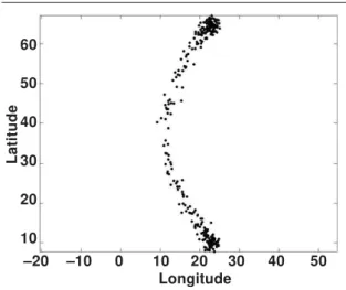
(latN – lat(t)) / (latN – latS) * (lonN – lon(t)) (2) to the longitude in order to create a curved migra-tion route (see figure 1). In addimigra-tion, to each lati-tude and longilati-tude value a random number from the normal distribution N(0,1) was added.
The population set consisted of 1,000 birds on each of 185 days. This population represents a fast migrant and the birds follow a curved and relatively narrow flyway with only a small position-date vari-ation. A sample of the simulated records is plotted in figure 1.
Example 1a
For this data set we drew two samples of sizes 100, and shifted one of the samples 3° to the east in order to create geographical difference between the two samples.
Example 1b
For this data set we drew two samples of sizes 100, and subtracted 5 days from all observations of one of the samples in order to create temporal differ-ence between the two routes.
Example 2
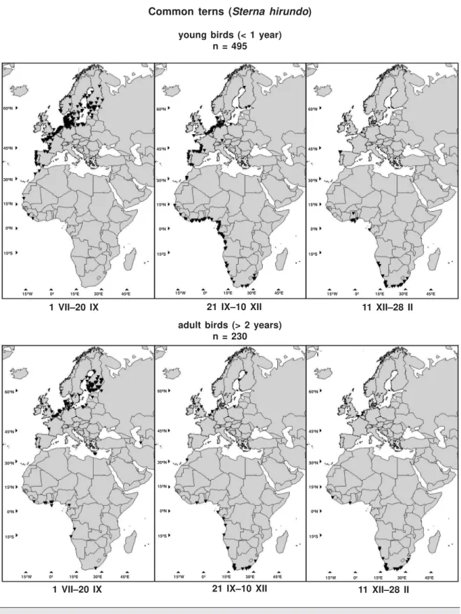
Recoveries of young (1 yr) and adult (+2 yr) Common terns (Sterna hirundo) ringed in Finland in 1930–2002 and encountered during 1 VII–28 II. Common terns follow closely the coast lines of Western Europe and Africa and the migration route includes curves and embodies large posi-tion–date variation. The 495 records of young and 230 records of adult Common terns are shown in figure 2. If (1) the date of the recovery is less accurate than 3 days, or (2) the place is
inaccurate, or (3) the condition of the bird is unknown, or (4) the bird had been dead for a long time, the recovery was excluded.
Example 3
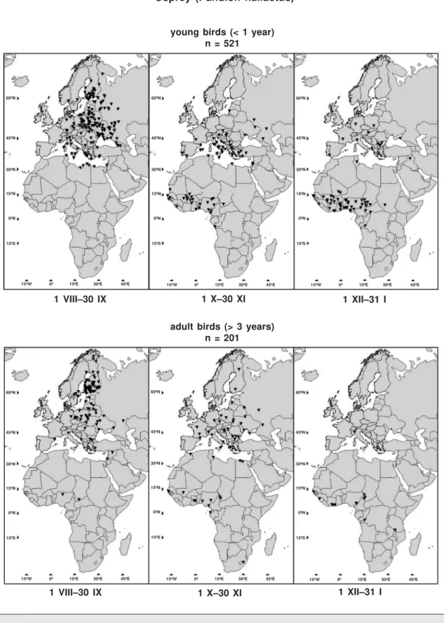
Recoveries of young (1 yr) and adult (+3 yr) Ospreys (Pandion haliaetus) ringed in Finland in 1932–2002 and encountered during 1 VIII–31 I. Ospreys migrate over a broad area and winter mainly in Western Africa but also in South Africa and the Mediterranean area. The 521 records of young and 201 records of adult Ospreys are shown in figure 3. The recoveries were selected according to the same criteria as in example 2. In addition we compared recoveries of young Os-preys reported "killed" and "found dead" along migration routes.
Re sult s
In this chapter we present results of examina-tions of the method for comparing timing and routes of migration. We also show how to distin-guish geographical difference from temporal
dif-Fig. 1. The shape of the migration route shown by randomly drawn 300 locations of the artificial data set 1. The geographical variation is due to a standard deviation of 1 degree in longitude and the temporal variation due to a standard deviation of 1 degree in latitude. Fig. 1. La forma de la ruta migratoria se indica mediante 300 emplazamientos dibuja-dos al azar del conjunto 1 de datos artificia-les. La variación geográfica obedece a la desviación estándar de un grado en longi-tud, mientras que la variación temporal obe-dece a la desviación estándar de un grado en latitud.
–20 –10 0 10 20 30 40 50
Longitude 60
50 40 30 20 10
1 VII–20 IX 21 IX–10 XII 11 XII–28 II
1 VII–20 IX 21 IX–10 XII 11 XII–28 II
60ºN
45ºN
30ºN
15ºN
0ºN
15ºS
15ºW 0º 15ºE 30ºE 45ºE
60ºN
45ºN
30ºN
15ºN
0ºN
15ºS
15ºW 0º 15ºE 30ºE 45ºE 60ºN
45ºN
30ºN
15ºN
0ºN
15ºS
15ºW 0º 15ºE 30ºE 45ºE
60ºN
45ºN
30ºN
15ºN
0ºN
15ºS
15ºW 0º 15ºE 30ºE 45ºE 60ºN
45ºN
30ºN
15ºN
0ºN
15ºS
15ºW 0º 15ºE 30ºE 45ºE 60ºN
45ºN
30ºN
15ºN
0ºN
15ºS
15ºW 0º 15ºE 30ºE 45ºE
Common terns (Sterna hirundo)
young birds (< 1 year) n = 495
Fig. 2. Locations of recoveries in the period of 1 VII–28 II of Common terns Sterna hirundo ringed in Finland in 1930–2002. In the period 11 XII–28 II a young bird found in Victoria, SE Australia, is not shown on the map.
Fig. 2. Localización de las recuperaciones correspondientes al período de 1 VII–28 II de charranes comunes Sterna hirundo anillados en Finlandia entre 1930 y 2002. En el periodo 11 XII–28 II un ave joven encontrada en Victoria, sudeste de Australia, no se indica en el mapa.
Fig. 3. Locations of recoveries in the period of 1 VIII–31 I of Ospreys Pandion haliaetus ringed in Finland in 1932–2002.
Fig. 3. Localización de las recuperaciones correspondientes al período de 1 VIII–31 I de águilas pescadoras Pandion haliaetus anilladas en Finlandia entre 1932 y 2002.
1 VIII–30 IX 1 X–30 XI 1 XII–31 I
1 VIII–30 IX 1 X–30 XI 1 XII–31 I
60ºN
45ºN
30ºN
15ºN
0ºN
15ºS
15ºW 0º 15ºE 30ºE 45ºE 60ºN
45ºN
30ºN
15ºN
0ºN
15ºS
15ºW 0º 15ºE 30ºE 45ºE 60ºN
45ºN
30ºN
15ºN
0ºN
15ºS
15ºW 0º 15ºE 30ºE 45ºE
60ºN
45ºN
30ºN
15ºN
0ºN
15ºS
15ºW 0º 15ºE 30ºE 45ºE 60ºN
45ºN
30ºN
15ºN
0ºN
15ºS
15ºW 0º 15ºE 30ºE 45ºE 60ºN
45ºN
30ºN
15ºN
0ºN
15ºS
15ºW 0º 15ºE 30ºE 45ºE
Osprey (Pandion haliaetus)
young birds (< 1 year) n = 521
ference in migration. Further we will show how to examine the differences in migration piece–wise in addition to the average difference over the entire migration period.
Distinguishing between geographical and temporal differences in migration routes and finding periods where differences occur
Examples 1a and 1b were created only to show how geographical difference can be distin-guished from difference of timing in migration. In analysis of example 1b we also show how periods of indication of difference in migration can be found.
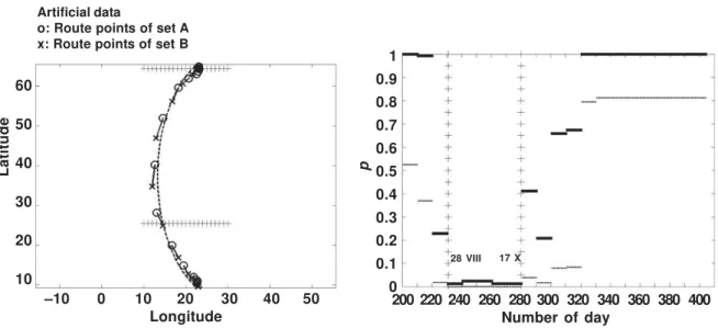
Figure 4 illustrates the analysis of example 1a. The points of the same dates of the two migration routes are connected at intervals of 5 days. When the reason for difference is the geographical deviation, the connecting lines are perpendicular to the migration direction as fig-ure 4 demonstrates.
Figure 5 illustrates the analysis of example
1b. In the left part the points of the same dates of the two migration routes are connected at intervals of 10 days. When the reason for differ-ence is the temporal deviation the connecting lines are parallel to the migration direction as figure 5 (left) demonstrates. In the right part are shown the original and multiplicity–adjusted p– values (denoted ) of piecewise analysis of data set 1b. As can be seen the probabilities that the null hypothesis hold are low in the period of 28 VIII–17 X and high elsewhere. The same time period is marked in the left part of figure 5. Comparison of migration routes of young and adult Common terns
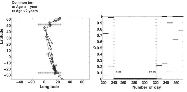
We compared the migration routes of young and adult Common terns (example 2 and figure 2). The observed value of the test statistic DS is located to the right of the empirical distribution of the test statistic (1,000 randomizations), giv-ing a very small p–value (p < 0.001). The differ-ence between the routes of young and adult Common terns is temporal because the lines joining the approximate positions at the same dates are parallel to the migration direction as can be seen in figure 6 (left). In figure 6 (right) are shown the results of the piece–wise test. In the period of 8 IX–26 XI the –values show that the null hypothesis should be rejected at signifi-cance level = 0.05. The same period is shown in the left part of figure 6. At the beginning of the migration of young and adult Common terns no indication of difference in timing was found, but soon after they have left Finland the young birds lag behind the adult ones until the routes con-verge time–wise in wintering areas in Southern Africa.
Comparison of migration routes of young and adult Ospreys
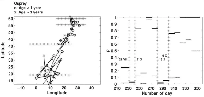
We compared the migration routes of young and adult Ospreys (example 3 and fig. 3). Only two values of the test statistic in 1,000 random-izations was above the observed value DS. Thus we reject the null hypothesis of similar routes of young and adult Ospreys at high significance level (p = 0.002). The observed difference in migration is illustrated in figure 7. In figure 7 (right) two sections can be localized where the null hypothesis should be rejected at signifi-cance level = 0.05: (1) at the beginning of migration in 29 VIII–7 IX and later in 18 X–6 XI. The sections are shown also in the left part of figure 7 where it can be seen that young Os-preys leave Finland earlier than adult ones, in most of Central Europe there is no difference in migration patterns of the two groups, but later adult Ospreys cross the Mediterranean and Sa-hara before the young birds. In the wintering area South of Sahara after 6 XI the recoveries do not show any difference.
Fig. 4. When two migration routes deviate geographically the lines connecting route points of the same dates are perpendicular to the migration direction. The migration direction is a Fourier curve fitted to the combined data of both sets of encounters. Fig. 4. Cuando dos rutas migratorias se desvían geográficamente, las líneas que conectan los puntos de la ruta de las mis-mas fechas son perpendiculares a la direc-ción de la migradirec-ción. La direcdirec-ción de la migración es una curva de Fourier ajustada a los datos combinados de ambos conjun-tos de hallazgos.
–20 –10 0 10 20 30 40 50
Longitude 60
50 40 30 20 10
Latitude
Artificial data
Comparison of recoveries of young Ospreys reported killed or found dead
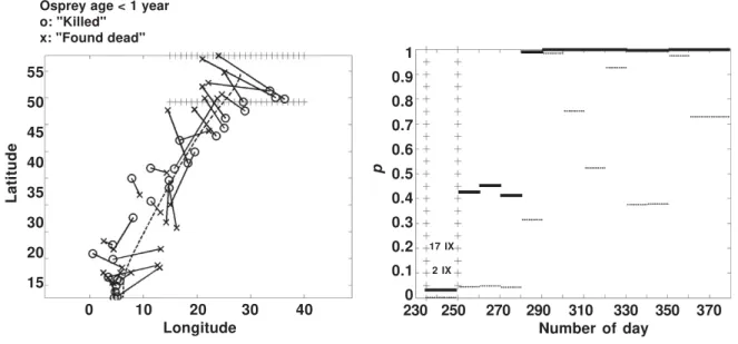
In figure 8 are shown the results of testing whether reported killing along the Osprey’s migration route varies. The data set contains 241 recoveries that were reported as "killed" and 274 recoveries of Ospreys reported as "found dead". The observed test statistic DS is in the middle of the empirical distribution of the test statistic (p = 0.54) and the null hypothesis cannot be rejected. However, in figure 8 (right) can be seen that in the period of 2 IX–17 IX the null hypothesis of the first time period should be rejected at significance level
= 0.05.
In figure 8 (left) can be seen that the lines joining the average positions of the same days are perpendicular to the migration direction indi-cating that the killing of Ospreys is emphasized in the South–Eastern part of the beginning of migration. We repeated the test to the same data where recoveries South of Sahara (or latitude 25) were excluded. This test indicated that the null
hypothesis must be rejected at a statistically highly significant level because the observed dif-ference DS was greater than all values in 1,000 randomizations.
Disc ussion
Geographical differences in sets of encounters have most often been studied in the literature as a two-sample location problem and it has been shown (Lokki & Saurola, 1987) that tests based on randomization perform well in this problem. Temporal differences have been studied separately for example by comparing arrival dates to a study location.
With the method introduced in this paper one can compare both geographical and temporal dif-ferences of two populations of encounters at the same time and later distinguish between the two causes of difference. In addition, the progress of migration can be studied in more detail in order to locate periods of differences along the migration route. In a way the method can be considered to be Fig. 5. When two migration routes deviate temporally the lines connecting route points of the same dates are parallel to the migration direction (left figure). The migration direction is a Fourier curve fitted to the combined data of both sets of encounters. In the section of 28 VIII–17 X, where the values < 0.05 the null hypothesis should be rejected at the significance level of = 0.05. The section is marked also in the left part of the figure (lines of + signs). In the right figure dotted segments of lines are the original and solid segments multiplicity–adjusted p–values .
Fig. 5. Cuando dos rutas migratorias se desvían temporalmente, las líneas que conectan los puntos de las rutas de las mismas fechas son paralelas a la dirección de la migración (figura de la izquierda). La dirección de la migración es una curva de Fourier ajustada a los datos combinados de ambos conjuntos de hallazgos. En la sección de 28 VIII–17 X, donde los valores < 0,05, la hipótesis nula debería rechazarse en el nivel de significación de = 0,05. La sección también está marcada en la parte izquierda de la figura (líneas de signos +). En la figura de la derecha, los segmentos punteados son los valores originales, mientras que los segmentos sólidos son los valores p ajustados para multiplicidad.
–10 0 10 20 30 40 50
Longitude 60
50 40 30 20 10
Latitude
1 0.9 0.8 0.7 0.6 0.5 0.4 0.3 0.2 0.1 0
200 220 240 260 280 300 320 340 360 380 400 Number of day
p
28 VIII 17 X
Artificial data
Fig. 6. Young and adult Common terns ringed in Finland start migration at the same time and follow the same geographical route. Later young birds lag behind adult ones. In the wintering area no geographical differences were found. The period 8 IX–26 XI, when the multiplicity–adjusted values < 0.05 indicating that the null hypothesis should be rejected, is marked in both left and right figures. In the right figure dotted segments of lines are the original and solid segments multiplicity–adjusted p– values .
Fig. 6. Los charranes comunes jóvenes y adultos anillados en Finlandia inician la migración a la vez y siguen la misma ruta geográfica. Posteriormente, las aves jóvenes van a la zaga de las adultas. En el área invernal no se encontraron diferencias geográficas. El período de 8 IX–26 XI, cuando los valores p ajustados para multiplicidad < 0,05 indican que la hipótesis nula debería rechazarse, está marcado tanto en la figura de la izquierda como en la de la derecha. En la figura de la derecha, los segmentos punteados son los valores originales, mientras que los segmentos sólidos son los valores p ajustados para multiplicidad.
–40 –20 0 20 40 60
Longitude 60
50 40 30 20 10 0 –10 –20 –30
Latitude
Common tern o: Age < 1 year x: Age >2 years
an extension to the two–sample location test based on randomization. Here the third dimension, in addition to the latitude and longitude, is time, which brings complexity to the analysis.
The migration route comparison method works in two phases, both of which are based on ap-proximations of the average daily positions. In the first phase the analyst computes the mean DS of the distances of the daily positions of the two routes. The test statistic DS is a mean. Therefore it is possible that a difference in one part of the migration route will not result in rejection of the null hypothesis, if in another part of the routes the daily positions are exceptionally close to each other. The comparison of "killed" and "found dead" young Ospreys is an example of this phenom-enon. In the second phase of the method these kinds of exceptional situations should be noticed. In the second phase the analyst follows the migra-tion routes piece–wise in time periods of k days and uses the mean of the distances of k days as test statistics. Correction for multiple testing was performed. By connecting the locations on the
same dates of the two routes the analyst can infer the cause of the observed difference: if the con-necting lines are perpendicular to the migration direction the reason for rejecting the null hypoth-esis is geographical and in case of temporal differ-ence the connecting lines are parallel to the migra-tion direcmigra-tion.
In the piece–wise examination we used periods of k = 10 days. If k ^ 10 the piece–wise test would lose power, because more tests would be per-formed and the correction for multiple testing would dilute the original p–values more. If k p 10 the test may fail to detect indications of short–term differ-ences but the power of the test rises. In our examples k = 10 was satisfactory because in all periods where the original p–values were < 0.05 at least part of the p–values corrected for multiple testing were also < 0.05.
What would be reasonable sizes of samples or sets of encounters? If one is analyzing migration routes that are several thousands of kilometers long, it is obvious that with only a few dozens of encounters the migration route will not be covered
1 0.9 0.8 0.7 0.6 0.5 0.4 0.3 0.2 0.1 0
220 240 260 280 300 320 340 360 Number of day
p
Fig. 7. Young Ospreys ringed in Finland seem to start migration before adult ones according to these data. It can be seen from the values < 0.05 in the period of 29 VIII–7 IX (right figure) and connecting lines of route points of the same period in the corresponding period in the left figure. In the mid–part of the migration (Central Europe) there is no indication of difference in the migration pattern of young and adult Ospreys which is illustrated by the –values in the period 8 IX–17 X (right figure). Later, in period 18 X–6 XI, the adult birds cross the Mediterranean and Sahara before young birds. This is seen from value < 0.05 in that period (right figure) and connecting lines of route points that are parallel to the migration direction (left figure). South of Sahara no evidence of different populations was found. In the right figure dotted segments of lines are the original and solid segments multiplicity–adjusted p– values .
Fig. 7. Según estos datos, las águilas pescadoras jóvenes anilladas en Finlandia parecen iniciar la migración antes que las adultas. Ello puede apreciarse por los valores < 0.05 en el período de 29 VIII– 7 IX (figura de la derecha) y las líneas de conexión de los puntos de la ruta del mismo período en el período correspondiente de la figura de la izquierda. En la parte central de la migración (Europa Central) no existe ninguna indicación de la diferencia en la pauta migratoria de las águilas pescadoras jóvenes y adultas, según lo ilustrado por los valores del período 8 IX–17 X (figura de la derecha). Posteriormente, en el período 18 X–6 XI, las aves adultas cruzan el mar Mediterráneo y el Sahara antes que las aves jóvenes. Ello puede apreciarse por el valor < 0,05 de ese período (figura de la derecha) y las líneas de conexión de los puntos de la ruta que son paralelas a la dirección de la migración (figura de la izquierda). Al sur del Sahara no se encontró ninguna evidencia de poblaciones distintas. En la figura de la derecha, los segmentos punteados son los valores originales, mientras que los segmentos sólidos son los valores p ajustados para multiplicidad.
well. Our tests of the route comparison method showed that the results are satisfactory even with sample sizes of 100 for even 10,000 km long routes.
What would be an optimal size of the sliding window? Our algorithm requires that a predefined minimum number of encounters must be included in each window. This adaptive nature of the window size means that the time span that the windows cover varies with the time spacing of the data. We have tested the method with window sizes of at least 10, 20 or 30 records in each window. When we compared the routes of young and adult Com-mon terns the sliding window of size m 30 recover-ies corresponds to a time window of 43 days on
average. Accordingly, in comparing routes of young and adult Ospreys the window size of m 30 records corresponds to a time window of 36 days on aver-age. It is possible that time windows covering such long periods of time are not flexible enough to follow the migration in sensible details. For exam-ple, in the Common tern case the comparison test would indicate temporal difference in migration in a longer period than in using a smaller window size. With a window size of m 10 recoveries in both cases of comparing routes of young and adult Common terns and Ospreys the corresponding time window is on average 15 days and the actual number of recoveries in the windows is on average 14–15. With these numbers the sliding window can follow
–10 0 10 20 30 40
Longitude 60
55 50 45 40 35 30 25 20 15
Latitude
Osprey o: Age < 1 year x: Age > 3 years
1 0.9 0.8 0.7 0.6 0.5 0.4 0.3 0.2 0.1 0
210 230 250 270 290 310 330 350 Number of day
p
the migration route in reasonable detail and at the same time the number of records in each window is reasonably high for computing the averages. So we conclude that a window size of the order of magni-tude 10 is preferable over a window size of 30 because a smaller time window is more flexible in following the migration and at the same time the number of encounters in each window is reason-ably high for computing means.
The Fourier analysis has been suggested for summarizing encounters in average position–date relation (Perdeck, 1977). We have fitted a partial sum of Fourier series with three harmonics to the data sets of this paper. These Fourier curves can roughly summarize geographical routes. The timing of migration is not followed with reasonable preci-sion because during migration the birds may pass some sections of the migration fast and then have lengthy stopovers. The sliding window technique can follow this pattern more closely than the Fourier curves that we have fitted. Adding more harmonics to the Fourier series may give a better fit.
When biologically interpreting the findings that the route comparison method produces, the ana-lyst must keep in mind the possible effects on
results that differences in recovery rates in differ-ent areas or periods of time may have. When the recoveries are generated by the general public and the routes are geographically close to each other, the recovery rates of both data sets are often roughly the same and the findings obtained by the method introduced in this paper are likely to reflect possible differences in migration of the two populations in question. When comparisons are made on the basis of ring recoveries generated by hunters the different hunting regulations in differ-ent areas must be taken into account. When en-counters of live birds are used, observations that are not independent must be excluded. Such records could be e.g. observations in a short period of time of the same individual in the same location.
Ac k now le dge m e nt s
We thank professor Carl Schwarz and an anony-mous referee for helpful comments, Marina Kurtén MA for checking the language and Heidi Björklund MSc for producing the maps of figures 2 and 3. Fig. 8. Young Ospreys’ recoveries are reported "killed" (n = 241) and "found dead" (n = 274) in different geographical areas in period of 2 IX–17 IX. In that period the values < 0.05 (right figure) and connecting lines of route points of the same dates are perpendicular to the migration direction (left figure). In the right figure dotted segments of lines are the original and solid segments multiplicity– adjusted p–values .
Fig. 8. Las recuperaciones de águilas pescadoras jóvenes se indican como "muertas" (n = 241) y como "encontradas muertas" (n = 274) en distintas áreas geográficas en el período de 2 IX–17 IX. En dicho período, los valores < 0,05 (figura de la derecha) y las líneas de conexión de los puntos de la ruta correspondientes a las mismas fechas son perpendiculares a la dirección de la migración (figura de la izquierda). En la figura de la derecha, los segmentos punteados son los valores originales, mientras que los segmentos sólidos son los valores p ajustados para multiplicidad.
0 10 20 30 40
Longitude 55
50 45 40 35 30 20 15
Latitude
Osprey age < 1 year o: "Killed"
x: "Found dead"
1 0.9 0.8 0.7 0.6 0.5 0.4 0.3 0.2 0.1 0
230 250 270 290 310 330 350 370 Number of day
p
17 IX
Re fe re nc e s
Bairlain, F., 2001. Results of bird ringing in the study of migration routes. Ardea, 89(1) (special issue): 7–19.
Batschelet, E., 1981. Circular Statistics in Biology. Academic Press.
Fransson, T. & Petterson, J., 2001. Swedish Bird Ringing Atlas (In Swedish with English summa-ries) Vol. 1. Stockholm.
Jenni, L. & Kéry, M., 2003. Timing of autumn bird migration under climate change: advances in long-distance migrants, delays in short–long-distance mi-grants. Proc. R. Soc. Lond. B, 270: 1467–1471. Lokki, H. & Saurola, P., 1987. Bootstrap methods
for two–sample location and scatter problems. Acta Ornithologica, 23(1): 133–147.
Munro, R. E. & Kimball, C. F., 1982. Population Ecology of the Mallard VII. Distribution and Deri-vation of the Harvest. U.S. Wildl. Serv. Resour. Publ., 147: 1–127.
Perdeck, A. C., 1977. The analysis of ringing data: pitfalls and prospects. Die Vogelwarte, 29 Sonderheft: 33–44.
Perdeck, A. C. & Clason, C., 1982. Flyways of Anatidae ringed in the Netherlands —an analysis based on ring recoveries. In: Proc. 2nd technical
meeting on Western Palearctic migratory bird man-agement, Paris 11–13 Dec. 1979: 65–88 (D. A. Scott & M. Smart, Eds.). Slimbridge, I.W.R.B. Perdeck, A. C. & Clason, C., 1983. Sexual
differ-ences on migration and winter quarters of ducks ringed in the Netherlands. Wildfowl., 34: 137– 143.
Saurola, P., 1978. Rengaslöytöjä tiirojen ja kihujen muuttoreittien varsilta. Lintumies, 13: 44–50. (In Finnish with English summary: Finnish recover-ies of Sterna and Stercorarius.)
Saurola, P., 1981. Varpushaukan muutto suoma-laisen rengastusaineiston kuvaamana. Lintumies, 16: 10–18 (In Finnish with English summary: Migration of the sparrowhawk Accipiter nisus as revealed by Finnish ringing and recovery data.) Sinnot, R. W., 1984. Virtues of the haversine. Sky
and telescope, 68(2): 159–170.