Contents lists available atScienceDirect
Expert Systems With Applications
journal homepage:www.elsevier.com/locate/eswa
A cooperative coevolutionary algorithm for the Multi-Depot Vehicle
Routing Problem
Fernando Bernardes de Oliveira
a,c, Rasul Enayatifar
a, Hossein Javedani Sadaei
a,
Frederico Gadelha Guimarães
b,∗, Jean-Yves Potvin
daGraduate Program in Electrical Engineering, Federal University of Minas Gerais, Av. Antônio Carlos 6627, 31270-901 Belo Horizonte, MG, Brazil bDepartment of Electrical Engineering, Universidade Federal de Minas Gerais, UFMG, Belo Horizonte, Brazil
cDepartamento de Computação e Sistemas, Universidade Federal de Ouro Preto, UFOP, João Monlevade, MG, Brazil
dCentre interuniversitaire de recherche sur les réseaux d’entreprise, la logistique et le transport (CIRRELT), Université de Montréal, C.P. 6128, succursale Centre-ville, Montréal, Québec, Canada H3C 3J7
a r t i c l e
i n f o
Keywords:
Multi-Depot Vehicle Routing Problem Vehicle routing
Cooperative coevolutionary algorithm Evolution strategies
a b s t r a c t
The Multi-Depot Vehicle Routing Problem (MDVRP) is an important variant of the classical Vehicle Routing Problem (VRP), where the customers can be served from a number of depots. This paper introduces a coop-erative coevolutionary algorithm to minimize the total route cost of the MDVRP. Coevolutionary algorithms are inspired by the simultaneous evolution process involving two or more species. In this approach, the prob-lem is decomposed into smaller subprobprob-lems and individuals from different populations are combined to create a complete solution to the original problem. This paper presents a problem decomposition approach for the MDVRP in which each subproblem becomes a single depot VRP and evolves independently in its do-main space. Customers are distributed among the depots based on their distance from the depots and their distance from their closest neighbor. A population is associated with each depot where the individuals rep-resent partial solutions to the problem, that is, sets of routes over customers assigned to the corresponding depot. The fitness of a partial solution depends on its ability to cooperate with partial solutions from other populations to form a complete solution to the MDVRP. As the problem is decomposed and each part evolves separately, this approach is strongly suitable to parallel environments. Therefore, a parallel evolution strategy environment with a variable length genotype coupled with local search operators is proposed. A large num-ber of experiments have been conducted to assess the performance of this approach. The results suggest that the proposed coevolutionary algorithm in a parallel environment is able to produce high-quality solutions to the MDVRP in low computational time.
© 2015 Elsevier Ltd. All rights reserved.
1. Introduction
A Vehicle Routing Problem (VRP) is a generic name for a large class of combinatorial optimization problems (Doerner & Schmid, 2010; Montoya-Torres, Franco, Isaza, Jiménez, & Herazo-Padilla, 2015). The goal is to find a set of routes for serving customers with a certain number of vehicles in a given environment. In the classical VRP, a problem instance is specified by a set of customers to be served with their corresponding locations and demands and other primary infor-mation such as distance between two costumers, distance between a customer and the depot, number of vehicles and vehicle capacity
∗ Corresponding author. Tel.: +55 3134093419.
E-mail addresses:[email protected](F.B. de Oliveira),
[email protected](R. Enayatifar),[email protected](H.J. Sadaei), [email protected],[email protected](F.G. Guimarães), [email protected](J.-Y. Potvin).
(Baldacci & Mingozzi, 2009). In a solution, each vehicle leaves the de-pot and executes a route over a certain number of customers before returning to the depot, while insuring that the total demand on the route does not exceed vehicle capacity. In some cases, a maximum route duration (or distance) constraint is enforced. The Multi-Depot Vehicle Routing Problem (MDVRP) is a variant of the classical VRP in which more than one depot is considered (Cordeau & Maischberger, 2012; Escobar, Linfati, Toth, & Baldoquin, 2014; Subramanian, Uchoa, & Ochi, 2013; Vidal, Crainic, Gendreau, Lahrichi, & Rei, 2012).
The number of studies on the MDVRP is rather limited when com-pared to the classical VRP. A survey of these studies, based on either exact methods or heuristics, can be found inMontoya-Torres et al. (2015). In recent years, evolutionary-based metaheuristics proved to be a popular approach to address this problem, as described in Section 3. But, in spite of this popularity, no coevolutionary algorithm has yet been proposed in the literature for the MDVRP. As the problem can be easily decomposed into a number of single-depot VRPs, with a
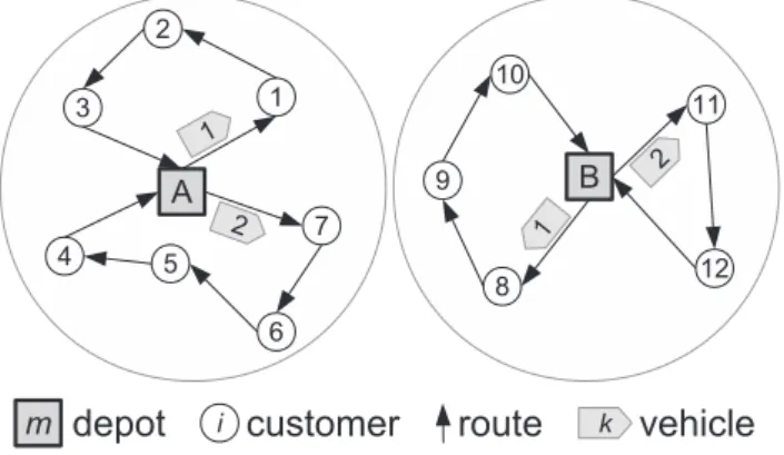
Fig. 1. MDVRP solution.
population of partial solutions associated with each depot, a coevolu-tionary approach looks relevant. Each partial solution or individual in a population corresponds to vehicle routes defined over the subset of customers assigned to the corresponding depot. Although each pop-ulation can evolve separately, this evolution is guided by the ability of each individual to form good complete solutions with individu-als from the other populations. This is the problem-solving approach proposed in this work.
The remainder of this paper is organized as follows. First, some preliminaries about the MDVRP and coevolution are found in Section 2.Section 3presents a literature review.Sections 4and5 de-scribe the proposed methodology whileSection 6reports computa-tional results. Future avenues for research are proposed in the con-clusion inSection 7.
2. Preliminaries
In this section, some preliminary information about the mathe-matical formulation of the MDVRP and cooperative coevolutionary algorithms are presented.
2.1. Multi-Depot Vehicle Routing Problem formulation
As mentioned earlier, the MDVRP is a variant of the classical VRP where more than one depot is considered (Montoya-Torres et al., 2015). Fig. 1 shows a typical solution of this problem with two depots and two vehicle routes associated with each depot. Typi-cally, the fleet of vehicles is limited and homogeneous (Cordeau & Maischberger, 2012; Escobar et al., 2014; Montoya-Torres et al., 2015; Subramanian et al., 2013; Vidal et al., 2012).
Basically, a solution to this problem is a set of vehicle routes such that: (i) each vehicle route starts and ends at the same depot, (ii) each customer is served exactly once by one vehicle, (iii) the to-tal demand on each route does not exceed vehicle capacity (iv) the maximum route time is satisfied and (v) the total cost is minimized (Montoya-Torres et al., 2015).
The MDVRP can be formalized as follows. LetG=
(
V,A)
be a com-plete graph, whereVis the set of nodes andAis the set of arcs. The nodes are partitioned into two subsets: the customers to be served,VC=
{1
, . . . ,N}
, and the multiple depots VD={
N+1, . . . ,N+M}
, withVC∪VD=VandVC∩VD= ⊘. There is a non-negative costcij as-sociated with each arc (i, j)∈A. The demand of each customer isdi (there is no demand at the depot nodes). There is also a fleet ofKidentical vehicles, each with capacityQ. The service time at each cus-tomeriistiwhile the maximum route duration time is set toT. A conversion factorwijmight be needed to transform the costcijinto time units. In this work, however, the cost is the same as the time and distance units, sowi j=1.
In the mathematical formulation that follows, binary variablesxijk are equal to 1 when vehiclekvisits nodejimmediately after nodei.
Auxiliary variablesyiare also used in the subtour elimination con-straints.
Minimize N+M
i=1
N+M
j=1
K
k=1
ci jxi jk, (1)
subject to:
N+M
i=1
K
k=1
xi jk=1
(
j=1, . . . ,N)
; (2)N+M
j=1
K
k=1
xi jk=1
(
i=1, . . . ,N)
; (3)N+M
i=1
xihk− N+M
j=1
xh jk=0
(
k=1, . . . ,K; h=1, . . . ,N+M)
; (4)N+M
i=1
N+M
j=1
dixi jk≤Q
(
k=1, . . . ,K)
; (5)N+M
i=1
N+M
j=1
ci jwi j+ti
xi jk≤T
(
k=1, . . . ,K)
; (6)N+M
i=N+1
N
j=1
xi jk≤1
(
k=1, . . . ,K)
; (7)N+M
j=N+1
N
i=1
xi jk≤1
(
k=1, . . . ,K)
; (8)yi−yj+
(
M+N)
xi jk≤N+M−1;for 1≤i=j≤Nand 1≤k≤K; (9)
xi jk∈
{
0,1} ∀
i,j,k; (10)yi∈
{
0,1} ∀
i; (11)The objective(1)minimizes the total cost. Constraints(2)and(3) guarantee that each customer is served by exactly one vehicle. Flow conservation is guaranteed through constraint(4). Vehicle capacity and route duration constraints are found in(5)and(6), respectively. Constraints(7)and(8)check vehicle availability. Subtour elimination constraints are in(9). Finally,(10)and(11)definexandyas binary variables.
In the original formulation of the MDVRP, a fixed number of ve-hicles is allocated to each depot. In our work, though, the search is allowed to consider a larger number of vehicles (at a penalty cost in the objective). This is discussed inSection 5.
2.2. Coevolutionary algorithms
Coevolutionary algorithms are a class of evolutionary algorithms inspired by the simultaneous evolution process involving two or more species. Recently, various engineering problems have been solved with this approach (Blecic, Cecchini, & Trunfio, 2014; Chen, Mori, & Matsuba, 2014; Ladjici & Boudour, 2011; Ladjici, Tiguercha, & Boudour, 2014; Wang & Chen, 2013a; Wang, Cheng, & Huang, 2014). Coevolutionary algorithms are categorized into two groups depend-ing on the type of interaction among the species, which can be either competitive or cooperative.Competitive coevolutioncan be viewed as anarms race, that is, individuals in the populations compete among themselves. One group attempts to take advantage over another, which responds with an adaptive strategy to recover the advantage (Katada & Handa, 2010). A biological example is thepredator–prey
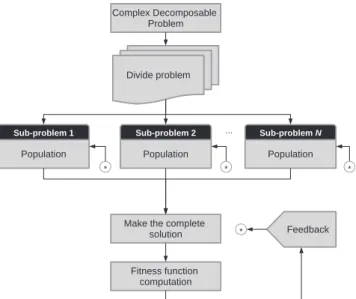
Fig. 2.Cooperative coevolutionary algorithm with problem decomposition.
affects the evolution of the other. This approach has been used in virtual and simulated evolution (Ebner, 2006) and also for evolving agent behaviors or artificial players for games (Engelbrecht, 2007). In cooperative coevolution, the interaction among species is bene-ficial for all or, at least, does not cause any damage. The species may live together in the same area and one population needs the other ones to survive and evolve. Typically, species cooperate to attain a global benefit. This is the case in symbiosis, for example Engelbrecht (2007).
In a cooperative coevolutionary algorithm, each population repre-sents a part of a complex decomposable problem (Engelbrecht, 2007). Accordingly, the true fitness of an individual can only be obtained from its interaction with other individuals from the same or other populations. Each individual receives a reward or punishment, be-ing rewarded when it interacts well with the others while gettbe-ing a punishment otherwise. A cooperative coevolutionary algorithm is considered in this work because the problem can be decomposed into smaller subproblems, each one evolving in parallel. Partial so-lutions for those subproblems cooperate to create a complete solu-tion for the MDVRP. In this situasolu-tion, a competitive strategy would not be suitable because a complete solution is obtained from infor-mation gathered from all subproblems and there is no competition among these subproblems.Fig. 2depicts a general cooperative coevo-lutionary algorithm with decomposition. A complex problem is first decomposed into smaller subproblems. Each population is evolved on its subproblem and, after a number of generations, individuals from these populations are combined to create complete solutions to the original problem. Through this process, it is possible to compute the fitness of these complete solutions. Some feedback information is then returned to each population, such as the best solution found so far, any required updates to the individuals in the population, etc.
Coevolutionary algorithms can be distinguished from traditional evolutionary algorithms by their evaluation process (Ficici, 2004). As mentioned above, individuals can only be evaluated through interac-tion with other individuals from the same or different populainterac-tions.
Fitness sampling(Engelbrecht, 2007) orfitness assessment(Luke, 2013) defines how individuals are combined for the purpose of fitness evaluation. These methods are the followings (Engelbrecht, 2007; Luke, 2013):
(a) All versus all. All possible combinations of individuals from all populations are considered. This method is very expensive and can be appropriate for populations with only a few individuals.
(b) Random. Individuals are randomly selected from the coevolv-ing populations. This method is less expensive than the previ-ous one and the number of evaluations is typically a parameter of the method.
(c) All versus best. All individuals of one population are combined with the best individuals from other populations. This is re-peated for each population.
(d) Tournament sampling. This process consists of selecting in-dividuals from each population based on their fitness. Then, a tournament is performed among all selected individuals to de-termine a winner. This is typically used in competitive models. (e) Shared sampling. Only individuals with higher shared fitness are combined to favor individuals that are significantly differ-ent from the others in a population.
3. Literature review
The literature review focuses on the main issues addressed in this work. First,Section 3.1introduces evolutionary-based algorithms for the MDVRP, followed by parallel algorithms for the MDVRP in Section 3.2. Then,Section 3.3is devoted to known applications of se-quential and parallel coevolutionary algorithms.
3.1. Heuristics for the Multi-Depot Vehicle Routing Problem
Evolutionary algorithms (EAs) use a set of candidate solutions, known as apopulation, and heuristic mechanisms to evolve it like
selectionandreproduction(also calledgenetic operators). Evolution proceeds from one generation to the next until a stopping condition is satisfied (Engelbrecht, 2007; Luke, 2013). Evolutionary algorithms have been widely used to solve the VRP, as surveyed inPotvin (2009). The main contributions with regard to the MDVRP are reported be-low.
Genetic algorithms (GAs) are probably the most widely used class of evolutionary algorithms and were applied as well to the MDVRP. A comprehensive survey of different types of GAs for the MDVRP can be found inKarakatiˇc and Podgorelec (2015), while GAs for the MDVRP, among other VRP variants, are also described inGendreau, Potvin, Bräumlaysy, Hasle, and Løkketangen (2008). With regard to hybrids, a simulated annealing-based solution acceptance criterion is applied after reproduction inChen and Xu (2008). The Clarke and Wright savings heuristic and the nearest neighbor heuristic are used inHo, Ho, Ji, and Lau (2008)to create initial solutions for the GAs. A combination of simulated annealing, bee colony optimization and GA is also proposed inLiu (2013).Vidal et al. (2012)andVidal, Crainic, Gendreau, and Prins (2014)introduce a powerful hybrid GA using neighborhood-based heuristics and population-diversity man-agement schemes to address many different types of VRPs, including the MDVRP.
Particle swarm optimization (PSO) is inspired by the social be-havior of agents, such as swarms and birds flock. Individuals are namedparticles, flyingin the search space according to simple rules that combine local and global information (Engelbrecht, 2007; Luke, 2013). This problem-solving methodology was used inWenjing and Ye (2010)for solving the MDVRP.
In addition to EAs, some noteworthy heuristics were proposed to solve the MDVRP. Tabu Search (TS) has been used in several contexts. In particular,Renaud, Laporte, and Boctor (1996)andCordeau, Gen-dreau, and Laporte (1997)use this heuristic for some VRP problems including MDVRP. A hybridgranularTS algorithm was proposed by Escobar et al. (2014). Those authors introduce the idea ofgranular neighborhoods, in which the search process uses restricted neighbor-hoods for each customer defined by agranularity threshold value.
The method developed bySubramanian et al. (2013)combines an exact procedure based on the set partitioning formulation with an Iterated Local Search (ILS). A Mixed Integer Programming solver is used for the exact procedure.
3.2. Parallel algorithms for the Multi-Depot Vehicle Routing Problem
A few parallel algorithms for the MDVRP are reported in the lit-erature. A parallel version of Ant Colony Optimization (ACO) is in-troduced inYu, Yang, and Xie (2011). In this work, the MDVRP was simplified through the definition of a single virtual depot, while in-suring that the capacity constraint of each vehicle is satisfied. The algorithm was implemented using a distributed coarse-grained en-vironment composed of eight computers each equipped with a Pen-tium processor (3 GHz with 512 MB RAM).
A parallel iterated Tabu Search (TS) is proposed inMaischberger and Cordeau (2011)andCordeau and Maischberger (2012). In the first paper, some preliminary results are reported on eight classes of VRPs including the MDVRP. The algorithm was run on a cluster made of 128 nodes (each with a 3 GHz Xeon processor). The second paper reports results over four VRP variants, including the MDVRP, as well as other variants with time windows.
3.3. Coevolutionary algorithms
In this section, we review different applications of CAs. Note that a discussion about sequential and parallel versions of CAs can be found inPopovici and De Jong (2006). The authors show in particular how different population update strategies can impact the overall perfor-mance. The authors empirically demonstrate the superiority of the parallel version over the sequential one on benchmark functions, us-ing a number of different metrics.
A competitive model with three populations is used in Li, Guimarães, and Lowther (2015)to solve constrained design problems. The first population is made of candidate solutions from the design space while the other populations represent disturbances due to un-certainties.Li and Yao (2012)propose a cooperative coevolutionary algorithm in a particle swarm environment. They apply it to large scale optimization problems on functions with up to 2000 variables. Other methodologies using particle swarm and coevolution can also be found inAote, Raghuwanshi, and Malik (2015)andChen, Zhu, and Hu (2010).
A study on sequential and parallel versions of a cooperative coevolutionary algorithms based on the ES(1+1) evolution strat-egy is presented in Jansen and Wiegand (2003) 2004). The au-thors identify situations where a cooperative scheme could be inappropriate, like problems involving non separable functions. Depending on the decomposition method or the characteris-tics of the function, the coevolutionary algorithm could even be harmful.
As far as we know, the coevolutionary paradigm has never been applied to the MDVRP. With regard to vehicle routing in general, a large scale capacitated arc routing problem is addressed inMei, Li, and Yao (2014)using a coevolutionary algorithm. In this work, the routes are grouped into different subsets to be optimized and prob-lem instances with more than 300 edges are solved. A multi-objective capacitated arc routing problem is also studied inShang et al. (2014). A coevolutionary algorithm is presented inWang and Chen (2013b) for a pickup and delivery problem with time windows. To minimize the number of vehicles and the total traveling distance, the authors use two populations: one for diversification purposes and the other for intensification purposes. In the scheduling domain, a competi-tive coevolutionary quantum genetic algorithm for minimizing the makespan of a job shop scheduling problem is reported inGu, Gu, Cao, and Gu (2010).
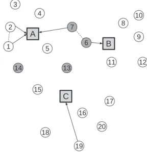
Fig. 3. Problem decomposition: assignment of customers to depots.
4. Cooperative coevolutionary model for the MDVRP
A cooperative coevolutionary model with problem decomposition is proposed here to solve the MDVRP. The main contribution of this method is the computational efficiency resulting from the decompo-sition of the problem into subproblems. Each subproblem becomes a single depot VRP and evolves independently in its domain space. The decomposition approach considers the depots separately and assigns a subset of customers to each one. Some overlap is possible, that is, customers might be associated with one or more depots depending on their neighbors (other customers or depots). An evolving popula-tion is associated with each subproblem and the (partial) solupopula-tions in each population must then cooperate to form a complete solution to the MDVRP. In this section, we explain the decomposition approach. Then,Section 5describes the evolution process for solving the sub-problems.
Each customer is assigned to a depot using the two following rules:
1. The closest depot.
2. The closest depot to the closest neighbor node (if different from the one in rule 1).
When the two rules identify the same depot, the assignment is obvious. When the two rules identify two different depots, then the conflict must be addressed in some way. Fig. 3 illustrates how these rules are applied. In the figure, there are three depots (nodes A–C) and 20 customers (nodes 1–20). For customer 1, rule 1 identifies A as the closest depot. Then, rule 2 identifies the clos-est neighbor to customer 1 as customer 2, whose closclos-est depot is also A. Thus, customer 1 can only be assigned to depot A. In the figure, all white nodes can only be assigned to their closest depot.
Now, let us consider customer 6. Rule 1 identifies B as the closest depot. Then, rule 2 identifies the closest neighbor to cus-tomer 6 as cuscus-tomer 7, whose closest depot is A. Since we do not know if it is better to assign customer 6 to depot A or B, cus-tomer 6 is initially assigned to both depots. That is, this cuscus-tomer will be part of the two evolving populations associated with de-pots A and B. It implies that there is some overlap among the sub-problems. In Fig. 3, all gray nodes are assigned to two different depots.
Algorithm 1:Assignment of customers.
1assignCustomers(VC,VD,A)
2 fori←1toNdo // for each customer i
// Rule 1: closest depot
3 mi←getClosestDepot(VD,i);
4 insert(Ami,i);
// Rule 2: depot of the closest neighbor
5 j←getClosestNeighbor(VC,i);
6 mj←getClosestDepot(VD,j);
7 if(mi=mj)then // Different depots
8 insert(Amj,i);
9 end if 10 end for
11 return(A1. . .AM);
12 end
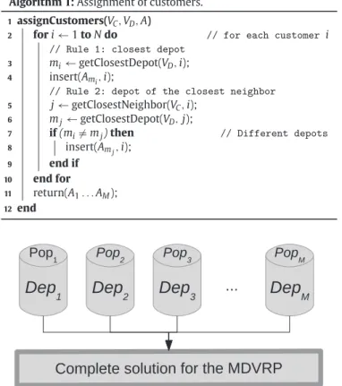
Fig. 4. Cooperative coevolutionary model for the MDVRP.
as well as the set of arcsA. In Line 3 the closest depotmito cus-tomeri is selected according to rule 1 and inserted in the assign-ment groupAmi of depotmi(Line 4). The closest neighbor to cus-tomeriis defined as customerj(Line 5) and the closest depot toj, identified asmj, is selected according to rule 2. The depots are com-pared in Line 7. If the two depots are different (mi=mj), customer
i is also inserted in the allocation groupAmj of depot mj(Line 8). After processing all customers, the assignment groups are returned (Line 11).
After this decomposition, each subproblem becomes a classi-cal single depot VRP for a subset of customers identified by the two assignment rules above. Given that the gray nodes are du-plicated, a repair operator will be needed to obtain a valid com-plete solution (see Section 5.5). Each subproblem is solved with an evolutionary algorithm, in which each individual represents a partial solution to the MDVRP. Fig. 4 illustrates the structure of the proposed coevolutionary model. For each depot, there is one population which evolves and searches the best routes for the set of customers assigned to it. Then, one individual for each population is selected to create a complete solution for the MDVRP.
A decomposition approach is particularly interesting for problem instances with a low degree of interdependency (coupling) between the subproblems. For example, customer 19 inFig. 3should clearly be served by depot C. It is unlikely that good solutions will be obtained by assigning this customer to depots A or B, and these solutions are automatically eliminated through the decomposition approach. It is clear that some degree of interdependency exists among the sub-problems for the instance illustrated inFig. 3, due to the presence of gray nodes.
This model is strongly suitable for a parallel environment where each population evolves separately and cooperates with other popu-lations to solve the problem. A parallel architecture for this model is proposed in the next section.
Algorithm 2:CoES—general scheme.
1 CoES(VC,VD,A,N,M,Q))
2 A1. . .AM←assignCustomers(VC,VD,A);
3 [P1. . .PM]←initializePopulations(A1. . .AM,μ,
α
);4 S←createCompleteSolutions(P1. . .PM);
5 f←evaluateSolutions(S);
6 s∗ ←getBestSolution();
7 startModules(); 8 return(s∗);
9 end
Fig. 5. Giant tour representation and the obtained routes.
5. Parallel evolution strategy
A parallel environment exploiting the evolution strategy (ES) paradigm, calledCoES, supports the evolution of our cooperative co-evolutionary model. Evolution strategy (Engelbrecht, 2007; Freitas, Guimarães, Pedrosa Silva, & Souza, 2014; Luke, 2013) is an evolution-ary algorithm usingmutationas the main operator to generate new solutions. ES was chosen because each subproblem has a variable length representation (genotype) and the design of a recombination operator in this case would be rather cumbersome (seeSection 5.2).
The proposed parallelization scheme, which is operational under
asynchronousupdates, is shown inAlgorithm 2. CoESfirst receives all required information about the problem, in particular the num-ber of customers (N), number of depots (M) and vehicle capacity (Q). Each population is initialized with
μ
individuals (Line 3), which are encoded using the representation scheme presented inSection 5.1. The initialization procedure uses a semi-greedy method to insert cus-tomers from a given list. Parameterα
defines the number of cus-tomers in this list, as discussed inSection 5.2. Complete solutions are then created with aRandomfitness sampling strategy (Engelbrecht, 2007) (Line 4). Here, individuals from each initial population are se-lected randomly to create complete solutions. It should be noted that another strategy is used in the following populations, as explained inSection 5.5. In Line 5, all complete solutions are evaluated and the best one is selected (Line 6). Then, a number of parallel modules are started (Line 7). At the end, the best complete solution to the MDVRP is returned (Line 8).The representation and initialization procedures are described in Sections 5.1 and 5.2. The parallel modules are introduced in Section 5.3.
5.1. Representation
Individuals from each population are represented by agiant tour, without route delimiters. It is basically a single sequence made of all customers assigned to a depot, as shown inFig. 5(a). Since each indi-vidual in a population corresponds to a particular depot and subset of customers, the length of the giant tour is likely to change ( vari-able genotype). Individual routes are created from this giant tour with theSplitalgorithm (Prins, 2004), which can optimally extract feasi-ble routes from a single sequence. In constrained profeasi-blems, theSplit
Algorithm 3:Populations initialization.
1initializePopulations(A1. . .AM,
μ,
α
)2 fori←1toMdo
3 forj←1to
μ
do4 if
(
j==1)
then// Greedy construction5 indj←greedy(Ai);
6 else// Semi-Greedy construction
7 indj←semiGreedy(Ai,
α
);8 end if
9 end for 10 insert(Pi,indj);
11 end for
12 end
Fig. 6. Architecture of the parallel modules inCoES.
converge toward feasible routes.Fig. 5(b) illustrates two routes that could be obtained from the giant tour representation in5(a).
5.2. Initialization
The population initialization procedure is shown inAlgorithm 3. The first individual in each population is constructed with the Nearest Insertion Heuristic (NIH) (Bodin, Golden, Assad, & Ball, 1983) while the other ones are constructed with a semi-greedy approach based on NIH. With regard to the first individual, the closest customer to the depot is first inserted in the giant tour. Then, the next customer to be inserted is the one which is closest to the previous one. This is repeated until the giant tour is complete.
Based on this greedy heuristic, a semi-greedy variant generates the remaining individuals. The first customer is selected at random. Then, the remaining customers are sorted based on their distance from the previous one. A restricted candidate list (RCL) is created with the
α
best-ranked customers and the next customer to be inserted is selected at random in the RCL. This is repeated until the giant tour is complete.5.3. Parallel modules and coordination
The parallel modules are executed until a stopping criterion, based on the execution time, is met.Fig. 6depicts the architecture of these modules withinCoESas well as their communication scheme.
TheStart Modulesprocedure is shown inAlgorithm 4. It is called in Line 7 ofAlgorithm 2to create a thread for each module and to initialize the environment. Astartflag is used to indicate that each module should wait until all modules have been initialized. At the beginning of the procedure, the flag is set toFALSE(Line 2). At the end, thestartflag is set toTRUE(Line 7) so that all modules can be executed.
TheMonitormodule manages the parallel processes and transmits information about the MDVRP problem. When the time-based
stop-Algorithm 4:Start Modules.
1 startModules() 2 start←FALSE;
3 createThread(Monitor()); 4 createThread(PE()); 5 createThread(CSE()); 6 createThread(EG()); 7 start←TRUE;
8 end
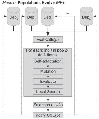
Fig. 7. Population Evolvemodule.
ping criterion is met, all modules are terminated by theMonitor mod-ule and the best solution is returned.
ThePopulation Evolve(PE) module evolves each population with ES. TheComplete Solutions Evaluate(CSE) module combines individ-uals from different populations to create and evaluate complete so-lutions. In addition, it applies local search heuristics to improve the complete solutions. TheElite Group(EG) module maintains an elite set of complete solutions, and also applies local search heuristics to these elite solutions. The various modules mentioned above are ex-plained in detail in the following sections.
5.4. Population Evolve (PE) module
ThePopulation Evolve(PE) module manages the ES-based evolu-tion by creating athreadfor each population. Within athread, the evo-lution process is run sequentially. This is represented inFig. 7. Note that the ES-based evolution is highlighted in the gray box ofFig. 7.
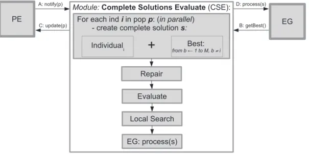
Fig. 8.Complete Solutions Evaluatemodule.
by swapping the corresponding customers. This is repeated
σ
times. Then, theSplitalgorithm is applied and individual routes are created, thus allowing for a local, population-based, fitness evaluation of the newly generated partial solution. With regard to fitness evaluation, the fixed number of vehicles at the depot is accounted for in different ways depending on the status of the parent. Basically, if this number is not exceeded in the parent, then its offspring incur a penalty cost for each vehicle in excess (if any). If this number is already exceeded in the parent, then no penalty is incurred in its offspring. With this approach, a mix of solutions with and without extra vehicles is main-tained throughout the search.A local search procedure is applied to the offspring with proba-bility
ρ
ls. Nine neighborhood structures are defined to improve theroutes. They are the same as those presented inPrins (2004),Vidal et al. (2012), andSiqueira Ruela et al. (2013). It is important to note that the local search is performed at the population or subproblem level, therefore only routes starting and ending at the depot and vis-iting the subset of customers in the subproblem are considered. Let us suppose thatuandvare two customer nodes belonging to the same or different routes,xis the successor ofuandyis the successor ofv
along their respective routes. The following moves are applied in ran-dom order, and the exploration of the corresponding neighborhood stops as soon as an improving move is found:
• Move 1: moveuafterv; • Move 2: move (u, x) afterv; • Move 3: move (x, u) afterv; • Move 4: exchangeuandv; • Move 5: exchange (u, x) withv; • Move 6: exchange (u, x) and (v, y);
• Move 7: if (u, x) and (v, y) are in the same route (but not adja-cent), replace them by (u, v) and (x, y);
• Move 8: if (u, x) and (v, y) are in distinct routes, replace them by (u, v) and (x, y);
• Move 9: if (u, x) and (v, y) are in distinct routes, replace them by (u, y) and (v, x).
Move 7 is a 2-opt move, while moves 8 and 9 are 2-opt∗moves. When all neighborhoods have been explored and no improvement to the current solution has been found, the local search procedure stops (Siqueira Ruela et al., 2013).
Once all offspring are created, parents and offspring are ranked ac-cording to their local fitness and the ES(
μ
+λ
) selection is applied to produce the next population. Using a producer–consumersynchro-Fig. 9.Repair procedure—remove duplicates.
nization scheme, the new population is then processed by the CSE module. The corresponding thread waits until the end of the evalua-tion of all complete soluevalua-tions before restarting.
5.5. Complete Solutions Evaluate (CSE) module
TheComplete Solutions Evaluatemodule receives a population of partial solutions from the PE module and evaluates the global fitness of complete solutions. Each complete solution is created and evalu-ated in amultithreadenvironment, where athreadis started for each individualiin populationp, as illustrated inFig. 8.
The CSE module is notified by the PE module to process popula-tionpat instant A inFig. 8. It combines each individual inpwith the best individuals obtained from the other populations to create a com-plete solution. More precisely, the partial solutions associated with the other depots are taken from the best solution in theElite Group
module (All versus beststrategy), see instant B inFig. 8.
Once a complete solution is created, a repair procedure is applied to remove duplicate customers and to insert customers that are not included in the solution. In both cases, theleast additional cost heuris-tic is used (Bodin et al., 1983). The additional cost when customeriis between customersxandyis defined inEq. (12). The least additional cost is looked for when inserting a customer between two consec-utive customers in the solution. When duplicates must be removed, only the copy with least additional cost is kept.
Cxiy=cxi+ciy−cxy (12)
To illustrate the removal of a duplicate customer, we refer toFig. 9 where customeriis included in two routes associated with depotsA
Fig. 10. Repair procedure—insert customer.
Fig. 11. Elite Groupmodule.
iis kept in the route of depot A and the duplicate is removed from the route of depot B.
When inserting a customer in a solution, all insertion positions between two consecutive customers are considered and the least cost one is chosen. InFig. 10, customeriis inserted between customersx
andyin a route of depotA.
The complete solution is evaluated and submitted to a local search procedure with probability
ρ
ls. The local search is based on the samemoves than those presented inSection 5.4. However, it is now pos-sible for a customer to be moved from one depot to another, thus changing individuals in the populations. This is the reason for the population update at instant C inFig. 8. After the update, the PE mod-ule is notified and can restart.
Each complete solution created is sent to the EG module at instant D inFig. 8. The module checks if the complete solution can be part of the elite group, as it is explained next.
5.6. Elite Group (EG) module
TheElite Group(EG) module maintains a set of
τ
elite complete solutions, including the best solution to the MDVRP found so far. This is illustrated inFig. 11. Assuming that a complete solution is submit-ted by the CSE module, the EG module will try to add the solution to the elite group. If there are less thanτ
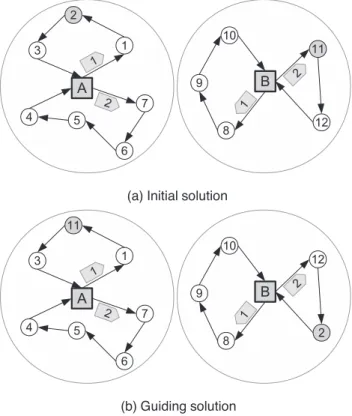
solutions in the elite group, the solution is automatically added. Otherwise, the new solution can enter the elite group only if it is better than the worst solution in the group, in which case it replaces the latter.The local search for the elite group operates in two steps, called PR and RI, where PR stands for Path Relinking and RI for Route Im-provement. The local search is run in amultithreadenvironment with athreadfor each solution in the elite group.
PR uses each solution in the elite group as aninitial solutionand the best solution so far as theguiding solution. To apply PR in this setting, the difference between aninitialsolutioniand theguiding
solutiongmust be calculated. We assume that each customer in a solution is characterized by the vehicle serving this customer and the corresponding depot. For each customer, the triplet (customer, depot,
(a) Initial solution
(b) Guiding solution
Fig. 12.Path-Relinking!.
vehicle) from the guiding solution is added to set
when it differs from the initial solution.We refer toFig. 12for an example. In this figure, we have one ini-tialsolution (Fig. 12a) and aguidingsolution (Fig. 12b). There are two depots A and B, 12 customers and two vehicles at each depot (rep-resented by the pentagons numbered 1 and 2). The difference be-tween the initial and guiding solutions corresponds to the nodes in gray, namely customers 2 and 11. Thus
={
(
2,B,2),(
11,A,1)
}. The
triplets inare then processed one by one to progressively modify the initial solution. That is, the customer in the first triplet is removed from its route in the initial solution and reinserted in the route indi-cated by the depot and vehicle of the guiding solution. A new solution is obtained which is closer to the guiding solution. The procedure is then applied again using the new solution and the second triplet. This is repeated until all triplets are done. It is hoped that a solution bet-ter than the guiding solution will emerge along the path between the initial and guiding solutions.The RI improvement procedure is applied to the solution returned by PR. This procedure is the local search mentioned inSection 5.5. If the solution obtained at the end is better than the best solution, then the elite group is updated.
6. Computational results
The performance of the proposed CoES algorithm was assessed through a number of computational experiments. They were con-ducted on the 33 MDVRP benchmark instances taken from the lit-erature (Cordeau et al., 1997; Cordeau & Maischberger, 2012; Escobar et al., 2014; Subramanian et al., 2013; Vidal et al., 2012).1These
in-stances are Euclidean and the time units are the same as the distance
Table 1
Selected parameter values.
Parameter Lower bound Upper bound
Tmax 600 s 1800 s Tupd 300 s 600 s
μ 20 100
τ 5 50
ρls 0.2 0.8
units. They are divided into S1 (P01−P23) and S2 (P24−P33)2and
have various sizes ranging from 48 to 360 customers, seeTable 4. The algorithm was implemented in C++ 113and all experiments
were run on a computer with two 2.50 GHz Intel Xeon (E5-2640) pro-cessors with 12 cores per CPU and 96 GB RAM. The computer was run under the Ubuntu 14.04.1 LTS operational system.
A first experiment was realized to set the parameter values, as it is discussed inSection 6.1. A comparison with the best solutions re-ported in the literature follows inSection 6.2.
6.1. Parameter settings
The algorithm stops when it reaches either the allowed total com-putation timeTmaxor the maximum computation time without im-provement to the best solutionTupd. Also, the number of individuals
μ
in each population and the maximum number of complete solu-tions in the elite groupτ
must be defined. Finally, the local search procedure in the PE and CSE modules are applied with a probabilityρ
ls.After some preliminary tests and using some values commonly found in the literature, lower and upper bound values were de-termined for the above parameters. These values are presented in Table 1.
As there are two values (levels) for each parameter (factors), a 2k factorial experiment was designed to study the impact of each fac-tor as well as their interactions. There are five facfac-tors with two lev-els each, resulting in 32 observations (25) for each instance. Selecting
the instance in group S1 (P01−P23) from the benchmark, we obtain a total of 736 observations (i.e., 32×23). Given the large number of factors and total observations, an experiment with a single repli-cation was performed. In this situation, theSparsity-of-effects princi-pleapplies, that is, the main effects and low-order interactions usu-ally dominate. Then, we can use an experiment with one replica-tion and combine highest-order interacreplica-tion for calculating the mean square error (Campelo, 2015, Chap. 12; Montgomery & Runger, 2011), The response variable corresponds to the gap between the solution value obtained by CoES and the best-known solution value reported inVidal et al. (2012).
The experiment is performed with the analysis of variance
(ANOVA) method from theR-Project(Core Team, 2015). Among other assumptions, ANOVA requires a normal distribution for the residuals. As the number of samples is large, they are approximately normal because of the Central Limit Theorem (CLT) and this assumption is satisfied.
Table 2reports only the significant factors and interactions identi-fied by ANOVA. In this case, the null hypothesis states that there is no significant impact and ap-value smaller than 0.05 invalidates this as-sumption.Table 2shows the significant factors identified by ANOVA along with their correspondingp-value.
Two main factors and one interaction have a significant impact on the results. The most significant factor is the number of individuals in each population
μ
. The second one is the elite group sizeτ
. The third2Those instances were proposed byCordeau et al. (1997)and they are also named pr01–pr10.
3C++ 2011 Standard.
Table 2
Significant factors and interac-tions.
Factor/interaction p-value
μ <2−16
τ 0.035
μ:ρls:τ 0.016
Table 3
Final parameter values.
Parameter Value
Tmax 1800 s Tupd 600 s
μ 20
τ 50
ρls 0.2
20
100
0 2 4 6 8
Number of individuals
10 50
0 2 4 6 8
Elite group size
Fig. 13. Boxplots of the two main factors.
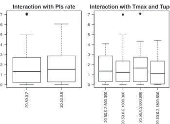
20.50.0.2 20.50.0.8
0 1 2 3 4 5 6 7
Interaction with Pls rate
20.50.0.2.600.300
20.50.0.2.1800.300 20.50.0.2.600.600 20.50.0.2.1800.600
0 1 2 3 4 5 6 7
Interaction with Tmax and Tupd
Fig. 14. Boxplots of interactions.
one corresponds to the interaction of the two previous factors with the local search rate
ρ
ls.Fig. 13shows box plots of the main factors.Based on these plots,
μ
was set to 20 andτ
was set to 50.Then, the other parameters can be set by fixing
μ
andτ
to the above values and by observing the interactions.Fig. 14shows box-plots of the interaction ofμ
=20 andτ
=50 withρ
ls,TmaxandTupd,respectively. The parameter values associated with the first two box-plots are shown in the format
μ.
τ.
ρ
ls. In the case of the four lastbox-plots, the format is
μ.
τ.
ρ
ls.Tmax.Tupd. The interaction betweenμ
,τ
Table 4
CoES(λ=μ): results.
Inst M N Q T Average values Best cost
Time (s) Cost
P01 4 50 80 ∞ 1.00 (*) 576.87 576.87 P02 2 50 160 ∞ 0.50 475.06 473.87 P03 3 75 140 ∞ 2.50 643.57 641.19 P04 8 100 100 ∞ 189.70 1011.42 1007.40 P05 5 100 200 ∞ 26.60 752.39 750.11 P06 6 100 100 ∞ 77.30 877.86 876.50 P07 4 100 100 ∞ 24.20 893.36 888.41 P08 14 249 500 310 803.40 4474.23 4450.37 P09 12 249 500 310 513.30 3904.92 3895.70 P10 8 249 500 310 719.90 3680.02 3666.35 P11 6 249 500 310 396.20 3593.37 3569.68 P12 5 80 60 ∞ 0.90 (*) 1318.95 1318.95 P13 5 80 60 200 0.00 (*) 1318.95 1318.95 P14 5 80 60 180 0.00 (*) 1360.12 1360.12 P15 5 160 60 ∞ 107.00 2549.65 2526.06 P16 5 160 60 200 8.20 (*) 2572.23 2572.23 P17 5 160 60 180 14.70 2733.80 2709.09 P18 5 240 60 ∞ 429.10 3781.66 3771.35 P19 5 240 60 200 72.60 (*) 3827.06 3827.06 P20 5 240 60 180 190.20 4094.86 4058.07 P21 5 360 60 ∞ 554.90 5668.97 5608.26 P22 5 360 60 200 214.00 5708.78 5702.16 P23 5 360 60 180 529.30 6159.90 6129.99
P24 1 48 200 500 0.00 849.17 849.17 P25 2 96 195 480 630.80 1271.39 1269.56 P26 3 144 190 460 123.60 1768.13 1759.77 P27 4 192 185 440 580.80 2057.50 2041.76 P28 5 240 180 420 321.00 2362.75 2314.72 P29 6 288 175 400 724.40 2690.01 2674.53 P30 1 72 200 500 0.60 (*) 1070.85 1070.85 P31 2 144 190 475 254.00 1650.96 1633.34 P32 3 216 180 450 652.50 2160.76 2139.78 P33 4 288 170 425 472.80 2844.32 2825.90
Average 261.70 2445.57 2432.67
S1 211.98 2694.69 2682.55
S2 376.05 1872.58 1857.94
The final parameter settings for the CoES algorithm are summa-rized inTable 3. The comparison with other algorithms in the next section is based on these parameter values.
6.2. Comparison with other methods
The performance of our CoES was compared with the best heuris-tics proposed for the MDVRP, namely, the Tabu Search (CGL) (Cordeau et al., 1997), the adaptive large neighborhood search (ALNS) (Pisinger & Ropke, 2007), a fuzzy logic guided genetic algorithm (FLGA) (Lau, Chan, Tsui, & Pang, 2010), a parallel iterated Tabu Search heuris-tic (ITS) (Cordeau & Maischberger, 2012), a hybrid algorithm com-bining Iterated Local Search and Set Partitioning (ILS-RVND-SP) (Subramanian et al., 2013), a hybrid genetic algorithm with adaptive diversity control (HGSADC+) (Vidal et al., 2014) and a hybrid Granular Tabu Search (ELTG) (Escobar et al., 2014).
CoES was run 10 times on all benchmark instances, using the pre-viously defined parameter settings. To remove any factor that could impact the performance, the order of execution of all replicates was randomized. Note that heuristics CGL and ELTG were run only once on each instance and the value reported was used to compare with the best value of CoES.
The results from CoES are shown inTable 4. The instance name is in columnInst, Mis the number of depots,Nis the number of cus-tomers,Qis the vehicle capacity andTis the maximum duration time of a vehicle route (∞means that there is no time constraint). The next two columns present the average values for the processing time (in seconds) and for the solution cost. When (∗) appears, the same
Table 5
CoES(λ=μ): comparison with results of the literature—best values.
Instance CGL ITS ILS-RVND-SP HGSADC+ ELTG
P01 0.00 0.00 0.00 0.00 0.00
P02 0.00 0.07 0.07 0.07 0.07
P03 −0.61 0.00 0.00 0.08 0.00
P04 0.07 0.64 0.64 0.82 0.64
P05 −0.43 0.01 0.01 0.01 0.01
P06 −0.15 0.00 0.00 0.00 0.00
P07 −0.40 0.73 0.73 0.73 0.42
P08 −0.72 1.41 1.62 1.77 1.80
P09 −0.64 0.90 0.94 0.96 0.38
P10 −1.30 0.97 0.96 0.97 1.01
P11 −0.31 0.62 0.67 0.67 0.69
P12 0.00 0.00 0.00 0.00 0.00
P13 0.00 0.00 0.00 0.00 0.00
P14 0.00 0.00 0.00 0.00 0.00
P15 −0.32 0.82 0.82 0.82 0.82
P16 0.00 0.00 0.00 0.00 0.00
P17 −0.41 0.00 0.00 0.00 0.00
P18 1.64 1.85 1.85 1.85 1.85
P19 0.00 0.00 0.00 0.00 0.00
P20 0.00 0.00 0.00 0.00 0.00
P21 1.31 2.44 2.44 2.44 2.44
P22 −0.24 0.00 0.00 0.00 0.00
P23 −0.16 0.84 0.84 0.84 0.57
P24 −1.41 −1.41 −1.41 −1.41 −1.41 P25 −3.45 −2.89 −2.89 −2.89 −3.17 P26 −3.08 −2.44 −2.44 −2.44 −2.44 P27 −2.51 −0.80 −0.80 −0.85 −1.08 P28 −3.88 −0.71 −0.71 −1.09 −1.49 P29 −3.38 −0.12 −0.23 −0.28 −1.32 P30 −1.95 −1.72 −1.72 −1.72 −1.72 P31 −2.56 −1.89 −1.89 −1.90 −1.93
P32 −1.70 0.31 0.31 0.26 −0.54
P33 −8.54 −1.82 −1.68 −2.10 −2.92
Average −1.06 −0.07 −0.06 −0.07 −0.22
S1 −0.12 0.49 0.50 0.52 0.47
S2 −3.25 −1.35 −1.35 −1.44 −1.80
solution was produced by CoES in each of the 10 runs. The last col-umn shows the best solution cost obtained by CoES.
The best and mean solution values, when compared with the other methods, are shown inTables 5and6, respectively. These ta-bles report thegap(in %), that is,
100×
(
ZCoES−Zlit)
ZlitwhereZCoESis the solution value of CoEs andZlitthe value of one of the other methods (as reported in the literature). A negative value indicates that CoES performs better. TheAverageline reports the av-eragegapover all instances. The linesS1andS2show the averagegap
over the instances in each subset. In the tables, the entries in bold in-dicate that the same or better solution values were obtained by CoES over the corresponding method.
With regard to the solutions reported inTable 4labeled with (∗), it should be noted that thegapwith the other methods inTable 6for those instances is always null (gap=0.00) or negative (gap<0.00). When considering the gap between CoES and the other methods in Table 6for the mean values, the average over all test instances is al-ways smaller than 0.5%. It is less than 0.9% for subset S1, while it is always negative for S2, indicating that CoES provides an improve-ment over each method in this case. When considering the gap in Table 5for the best values, the average over all test instances is al-ways negative. It indicates that CoES provides an improvement over every method. The trend observed for the mean values is also ob-served here: there is generally a positive gap in the case of subset S1, but a more important negative gap for S2. Thus, we conclude that CoES performs better on subset S2.
Table 6
CoES(λ=μ): comparison with results of the literature—mean values.
Instance CGL ALNS FLGA ITS ILS-RVND-SP HGSADC+ ELTG
P01 0.00 0.00 0.00 0.00 0.00 0.00 0.00
P02 0.25 0.32 0.32 0.32 0.32 0.32 0.32
P03 −0.25 0.37 0.37 0.37 0.37 0.46 0.37
P04 0.47 0.53 0.98 1.01 1.04 1.08 1.04
P05 −0.13 0.01 0.04 0.31 0.29 0.31 0.31
P06 0.00 −0.58 −0.55 0.16 0.16 0.16 0.16
P07 0.16 0.45 0.61 1.29 1.29 1.29 0.98
P08 −0.18 1.20 0.81 1.60 1.83 2.07 2.35
P09 −0.41 0.32 −0.29 0.92 1.05 1.14 0.62
P10 −0.93 0.36 0.28 1.17 1.25 1.33 1.39
P11 0.35 0.56 0.32 1.27 1.33 1.30 1.36
P12 0.00 −0.01 0.00 0.00 0.00 0.00 0.00
P13 0.00 0.00 0.00 0.00 0.00 0.00 0.00
P14 0.00 0.00 0.00 0.00 0.00 0.00 0.00
P15 0.61 1.19 1.42 1.77 1.77 1.77 1.77
P16 0.00 −0.07 −0.24 0.00 0.00 0.00 0.00
P17 0.50 0.91 0.91 0.91 0.87 0.91 0.91
P18 1.92 1.21 1.43 2.13 2.13 2.13 2.13
P19 0.00 −0.30 −0.35 0.00 −0.01 0.00 0.00
P20 0.91 0.74 0.78 0.91 0.91 0.91 0.91
P21 2.40 3.04 2.59 3.55 3.55 3.55 3.55
P22 −0.13 −0.23 −0.42 0.12 0.05 0.12 0.12
P23 0.33 1.10 1.00 1.33 1.33 1.31 1.06
P24 −1.41 −1.41 −1.41 −1.41 −1.41 −1.41 −1.41 P25 −3.32 −2.75 −3.16 −2.75 −2.84 −2.75 −3.03 P26 −2.62 −2.10 −2.30 −2.00 −1.99 −1.98 −1.98 P27 −1.75 −0.17 −0.90 −0.17 −0.17 −0.04 −0.32
P28 −1.88 1.07 −1.20 1.09 1.05 1.35 0.56
P29 −2.82 0.09 −1.43 0.26 0.18 0.51 −0.75
P30 −1.95 −1.72 −1.72 −1.72 −1.72 −1.72 −1.72 P31 −1.51 −0.83 −0.94 −0.87 −0.85 −0.83 −0.87
P32 −0.74 1.14 0.40 1.02 1.19 1.29 0.43
P33 −7.94 −1.57 −2.58 −1.47 −1.32 −0.83 −2.28
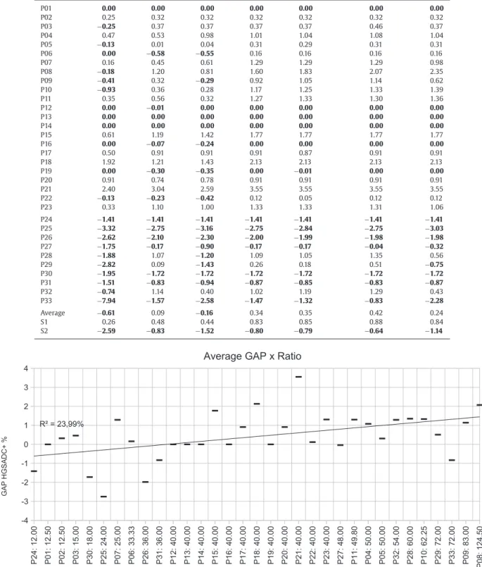
Average −0.61 0.09 −0.16 0.34 0.35 0.42 0.24
S1 0.26 0.48 0.44 0.83 0.85 0.88 0.84
S2 −2.59 −0.83 −1.52 −0.80 −0.79 −0.64 −1.14
Fig. 15. Average gap based on the ratio between customers and depots.
reference.Fig. 15shows the average gap with HGSADC+ when the in-stances are sorted in increasing order of the ratio between the num-ber of customers and the numnum-ber of depots. The graph presents a subtle trend suggesting that increasing the number of customers in each subproblem could make the problem harder for CoES. How-ever, the correlation factor isR2=23.99% and needs to be further
investigated.
Fig. 16. Average gap based on the ratio between customer assignments and depots.
Overall, the coevolution paradigm was able to produce compet-itive solutions, even if its inherent parallel nature was not fully ex-ploited in our implementation.
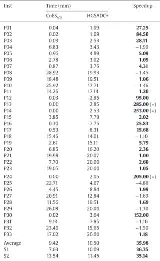
6.3. Comparison of CPU times
In order to compare the CPU times between the method proposed in this paper and HGSADC+ (Vidal et al., 2014), a conversion proce-dure is required. The performance of several computers is reported byDongarra (2014)when solving dense systems of linear equations. This conversion uses the amount of floating point operations per sec-ond (flop/s) as reference and the measure is estimated using the LIN-PACK Benchmark(Dongarra, 2014). The processor used inVidal et al. (2014)(AMD Opteron 250 2.4 GHz) is reported with 1291 Mflop/s. This value is computed with a matrix of order 100 (defined as prob-lem size). However, the environment used in our work is not reported and an experiment was conducted to obtain the (flop/s) under the same conditions. TheLINPACK Benchmarkwas obtained from Intel4
and a test was performed using 100 equations (problem size) and 100 trials. The average result of this test is 2787 Mflop/s. Therefore, a scal-ing factor of 2.16 is obtained by dividscal-ing 2787 Mflop/s by the reported value of 1291 Mflop/s inVidal et al. (2014).
Table 7shows the run times of our method (in minutes) in contrast to the run times reported for HGSADC+, considering the conversion factor. The column CoESadjcorresponds to the adjusted time for our method. The average times in seconds CoESsecreported inTable 4,
columnTime(s), were transformed into the corresponding adjusted values (in minutes) as follows:
CoESadj
(
min)
=CoESsec×2.16
60
The columnHGSADC+is the average computation time in minutes of HGSADC+. The speed-upSis calculated differently depending if CoES or HGSADC+ is faster:
S=Slower Faster
The ratio is positive when CoEs is faster. However, when HGSADC+ is faster, a minus sign is put in front ofSto get a negative ratio.
4Available at:http://goo.gl/1ZEYbj.
Table 7
Comparison of run time.
Inst Time (min) Speedup
CoESadj HGSADC+
P01 0.04 1.09 27.25
P02 0.02 1.69 84.50
P03 0.09 2.53 28.11
P04 6.83 3.43 −1.99
P05 0.96 4.89 5.09
P06 2.78 3.02 1.09
P07 0.87 3.75 4.31
P08 28.92 19.93 −1.45
P09 18.48 19.51 1.06
P10 25.92 17.71 −1.46
P11 14.26 17.14 1.20
P12 0.03 2.85 95.00
P13 0.00 2.85 285.00(∗)
P14 0.00 2.53 253.00(∗)
P15 3.85 7.79 2.02
P16 0.30 7.75 25.83
P17 0.53 8.31 15.68
P18 15.45 14.01 −1.10
P19 2.61 15.11 5.79
P20 6.85 16.20 2.36
P21 19.98 20.07 1.00
P22 7.70 20.00 2.60
P23 19.05 20.00 1.05
P24 0.00 2.05 205.00(∗)
P25 22.71 4.67 −4.86
P26 4.45 8.84 1.99
P27 20.91 12.84 −1.63
P28 11.56 19.51 1.69
P29 26.08 20.00 −1.30
P30 0.02 3.04 152.00
P31 9.14 7.85 −1.16
P32 23.49 15.65 −1.50
P33 17.02 20.00 1.18
Average 9.42 10.50 35.98
S1 7.63 10.09 36.35
S2 13.54 11.45 35.14
7. Conclusion and future work
This paper proposed a cooperative coevolutionary algorithm to solve the MDVRP. In this algorithm, each depot is associated with a population with its assigned customers. Individuals in each popu-lation represent partial single-depot solutions to the problem. Each population evolves separately, but the quality of an individual de-pends on its ability to cooperate with partial solutions from other populations to form a good complete solution to the MDVRP.
The results show that our coevolutionary algorithm produces competitive solutions when compared with the best known so-lutions, even improving some of them. Besides, it is faster than HGSDAC+, which is the best method reported in the literature. The benefit of our approach comes from its ability to decompose complex problems into simpler subproblems and evolve solutions to the subproblems in parallel. The decomposition approach also makes the method more scalable. In large MDVRP instances, it is unlikely that customers close to a depot will be allocated to a distant depot. Therefore, the coevolutionary algorithm incorporates important characteristics of a problem instance and allows a reduc-tion of the search space. Moreover, the evolureduc-tionary engine leads to simpler representations and genetic operators. Finally, the coevolu-tionary algorithm proposed in this work would greatly benefit from cloud computing architectures, cluster computing and GPU program-ming.
One interesting avenue of research would be to integrate math-ematical programming into the local searches (matheuristic). Since each subproblem reduces to a single-depot VRP, the use of math-ematical programming within each population could be beneficial. Additionally, other sophisticated local search strategies could be in-corporated into the EG module, like Tabu Search. Finally, we intend to improve the parallel implementation by exploiting GPU program-ming for the PE, CSE and EG modules.
Acknowledgments
F. B. Oliveira would like to thank the financial support fromCAPES Foundation, Ministry of Education of Brazil, grantBEX 0295/14-0, for awarding the scholarship for the visit period at CIRRELT in Université de Montréal.
R. Enayatifar and H. Javedani Sadaei would like to thank the sup-port given by the Brazilian Agency CAPES.
F. G. Guimarães would like to thank the support given by the National Council for Scientific and Technological Development(CNPq grant no.312276/2013-3), Brazil.
J.-Y. Potvin would like to thank the Natural Sciences and En-gineering Research Council of Canada (NSERC) for its financial support.
References
Aote, S., Raghuwanshi, M., & Malik, L. (2015). A new particle swarm optimizer with cooperative coevolution for large scale optimization. In S. C. Satapathy, B. N. Biswal, S. K. Udgata, & J. Mandal (Eds.),Proceedings of the third international conference on frontiers of intelligent computing: Theory and applications (FICTA) 2014. InAdvances in intelligent systems and computing: vol. 327(pp. 781–789). Springer International Publishing. doi:10.1007/978-3-319-11933-5_88.
Baldacci, R., & Mingozzi, A. (2009). A unified exact method for solving different classes of vehicle routing problems.Mathematical Programming, 120(2), 347–380. doi:10.1007/s10107-008-0218-9.
Blecic, I., Cecchini, A., & Trunfio, G. A. (2014). Fast and accurate optimization of a GPU-accelerated {CA} urban model through cooperative coevolutionary particle swarms.Procedia Computer Science, 29(0), 1631–1643. 2014 International confer-ence on computational sciconfer-encehttp://dx.doi.org/10.1016/j.procs.2014.05.148. Bodin, L., Golden, B., Assad, A., & Ball, M. (1983). Routing and scheduling of vehicles and
crews: The state of the art.Computers & Operations Research, 10(2), 63–211.
Campelo, F. (2015). Lecture notes on design and analysis of experiments. Version 2.11, creative commons BY-NC-SA 4.0. https://github.com/fcampelo/Design-and-Analysis-of-Experiments.
Chen, H., Mori, Y., & Matsuba, I. (2014). Solving the balance problem of massively multi-player online role-playing games using coevolutionary programming.Applied Soft Computing, 18(0), 1–11.http://dx.doi.org/10.1016/j.asoc.2014.01.011.
Chen, H., Zhu, Y., & Hu, K. (2010). Discrete and continuous optimization based on multi-swarm coevolution.Natural Computing, 9(3), 659–682. doi: 10.1007/s11047-009-9174-4.
Chen, P., & Xu, X. (2008). A hybrid algorithm for multi-depot vehicle routing problem. InIEEE international conference on service operations and logistics, and informatics, 2008. IEEE/SOLI 2008: vol. 2(pp. 2031–2034). doi:10.1109/SOLI.2008.4682866. Cordeau, J.-F., Gendreau, M., & Laporte, G. (1997). A tabu search heuristic for periodic
and multi-depot vehicle routing problems.Networks, 30(2), 105–119.
Cordeau, J.-F., & Maischberger, M. (2012). A parallel iterated tabu search heuristic for vehicle routing problems.Computers & Operations Research, 39(9), 2033–2050. http://dx.doi.org/10.1016/j.cor.2011.09.021.
Core TeamR. (2015).R: A language and environment for statistical computing. Vienna, Austria: R Foundation for Statistical Computing.
Doerner, K., & Schmid, V. (2010). Survey: Matheuristics for rich vehicle routing prob-lems. In M. Blesa, C. Blum, G. Raidl, A. Roli, & M. Sampels (Eds.),Hybrid metaheuris-tics. InLecture notes in computer science: vol. 6373(pp. 206–221). Berlin, Heidelberg: Springer. doi:10.1007/978-3-642-16054-7_15.
Dongarra, J. J. (2014).Performance of various computers using standard linear equations software (Linpack benchmark report).Technical report, CS-89-85.University of Ten-nessee Computer Science.
Ebner, M. (2006). Coevolution and the red queen effect shape virtual plants.Genetic Programming and Evolvable Machines, 7, 103–123. doi:10.1007/s10710-006-7013-2. Engelbrecht, A. (2007).Computational intelligence: An introduction. Wiley.
Escobar, J., Linfati, R., Toth, P., & Baldoquin, M. (2014). A hybrid granular tabu search algorithm for the multi-depot vehicle routing problem.Journal of Heuristics, 20(5), 483–509. doi:10.1007/s10732-014-9247-0.
Ficici, S. G. (2004).Solution concepts in coevolutionary algorithms. Waltham, MA, USA: (Ph.D. thesis). Faculty of Brandeis University.AAI3127125
Freitas, A. R. R., Guimarães, F. G., Pedrosa Silva, R. C., & Souza, M. J. F. (2014). Memetic self-adaptive evolution strategies applied to the maximum diversity problem. Op-timization Letters, 8(2), 705–714. doi:10.1007/s11590-013-0610-0.
Gendreau, M., Potvin, J.-Y., Bräumlaysy, O., Hasle, G., & Løkketangen, A. (2008). Meta-heuristics for the vehicle routing problem and its extensions: A categorized bibli-ography. In B. Golden, S. Raghavan, & E. Wasil (Eds.),The vehicle routing problem: Latest advances and new challenges. InOperations research/computer science inter-faces: vol. 43(pp. 143–169). US: Springer. doi:10.1007/978-0-387-77778-8_7. Gu, J., Gu, M., Cao, C., & Gu, X. (2010). A novel competitive co-evolutionary quantum
genetic algorithm for stochastic job shop scheduling problem.Computers & Opera-tions Research, 37(5), 927–937. Disruption managementhttp://dx.doi.org/10.1016/ j.cor.2009.07.002.
Ho, W., Ho, G. T., Ji, P., & Lau, H. C. (2008). A hybrid genetic algorithm for the multi-depot vehicle routing problem.Engineering Applications of Artificial Intelligence, 21(4), 548–557.http://dx.doi.org/10.1016/j.engappai.2007.06.001.
Jansen, T., & Wiegand, R. (2003). Sequential versus parallel cooperative coevolutionary (1+1) EAS. InThe 2003 congress on evolutionary computation, 2003. CEC ’03: vol. 1 (pp. 30–37). doi:10.1109/CEC.2003.1299553.
Jansen, T., & Wiegand, R. P. (2004). The cooperative coevolutionary (1+1) EA. Evolution-ary Computation, 12(4), 405–434.
Karakatiˇc, S., & Podgorelec, V. (2015). A survey of genetic algorithms for solving multi depot vehicle routing problem.Applied Soft Computing, 27(0), 519–532. http://dx.doi.org/10.1016/j.asoc.2014.11.005.
Katada, Y., & Handa, Y. (2010). Tracking the red queen effect by estimating features of competitive co-evolutionary fitness landscapes. In2010 IEEE congress on evolution-ary computation (CEC)(pp. 1–8). doi:10.1109/CEC.2010.5586188.
Ladjici, A., & Boudour, M. (2011). Nash–Cournot equilibrium of a deregulated electric-ity market using competitive coevolutionary algorithms.Electric Power Systems Re-search, 81(4), 958–966.http://dx.doi.org/10.1016/j.epsr.2010.11.016.
Ladjici, A., Tiguercha, A., & Boudour, M. (2014). Nash equilibrium in a two-settlement electricity market using competitive coevolutionary algorithms. International Journal of Electrical Power & Energy Systems, 57(0), 148–155. http://dx.doi.org/10.1016/j.ijepes.2013.11.045.
Lau, H., Chan, T., Tsui, W., & Pang, W. (2010). Application of genetic algorithms to solve the multidepot vehicle routing problem.IEEE Transactions on Automation Science and Engineering, 7(2), 383–392. doi:10.1109/TASE.2009.2019265.
Li, M., Guimarães, F., & Lowther, D. A. (2015). Competitive co-evolutionary algorithm for constrained robust design.IET Science, Measurement & Technology, 9(2), 218–223. doi:10.1049/iet-smt.2014.0204.
Li, X., & Yao, X. (2012). Cooperatively coevolving particle swarms for large scale optimization. IEEE Transactions on Evolutionary Computation, 16(2), 210–224. doi:10.1109/TEVC.2011.2112662.
Liu, C.-Y. (2013). An improved adaptive genetic algorithm for the multi-depot vehicle routing problem with time window.Journal of Networks, 8(5), 1035–1042. Luke, S. (2013). Essentials of metaheuristics (2nd). Lulu. Available for free at
http://cs.gmu.edu/˜sean/book/metaheuristics/