Disturbance of patterns in EEG spatial
correlations
∗
Tanya Ara´
ujo
†and A.Martins da Silva
‡Research Unit on Complexity in Economics (UECE)
ISEG, Universidade T´ecnica de Lisboa
Hospital Santo Ant´onio and ICBAS/IBMC
University of Porto, Porto
December 17, 2006
Abstract
In the study of epileptic seizure or epileptic attack , a strategy re-ceiving increased attention is the use of nonlinear methods in detecting the earliest dynamical changes preceding seizures. The methods usu-ally consider continuous EEG measurements from epileptic patients to predict and ultimately control seizures. As part of the inquiry into the structure of the dynamics of the brain activity we investigate changes amongst the EEG signals being recorded at different locations on the scalp. Patterns emerging from the correlation coefficients between the EEG channels seem to be disturbed with the approach of a crisis. Re-sults show that those patterns are often disturbed 10 to 15 minutes before the beginning of crises, helping to detect the earliest dynamical changes preceding seizures.
Keywords: EEG spatial correlations, epileptic seizures
∗Grant from BICE Tecnifar 2004-05 and 2005-06
1
Introduction
Using a metric related to the correlation coefficients between activities of pairs of EEG channels, a method is proposed to reconstruct characteristic patterns of correlation from the EEG data. The method was applied to seizure and normal activity recorded from scalp electrodes in epileptic pa-tients. Patterns of characteristic time delays were identified from the obser-vation of synchronous behavior between EEG channels, assembled in mono or bipolar derivations. Those patterns, which can be observed along both epileptic seizure and normal epochs, allowed for the classification of the pairs of channels into either weakly or strongly correlated ones. Few minutes be-fore the EEG seizure initiation the characteristic time delays remain almost unchanged for the strongly correlated channels, while some weakly corre-lated pairs of channels display interesting changes in their typical time de-lays. Disturbance of the behavior of the characteristic time delays for weakly correlated channels was observed in 20 out of 22 patients. Our results do suggest the existence of a well defined structure in the space defined by the correlation coefficients between EEG channels and their typical time delays. Moreover, results also show that disturbance in that correlation structure is empirically related to the beginning of a seizure; suggesting that, some weakly correlated pairs of channels may display a different pattern of synchronous coupling when a seizure approaches.
2
Data collection
3
Method
Consider EEG signals recorded at 16 different locations on the scalp over some time interval as Fig.1 shows.
Fp1 Fp2
F7
T3
T5
F3
C3
P3
O1 O2
5
6
7
8 13
14
15
16
F4 F8
Cz
P4 C4 T4
T6
1 9
2
3
4 10
11
12
Figure 1: Monopolar Montage and Channel Numeration
The idea is simply stated in the following terms:
1. Plot the individual signals recorded at the 16 EEG channels.
2. Classify the set of EEG signals accordingly to the synchronization pat-tern being observed from the plots.
In those cases, the EEG patient is referred to as being a module-k pa-tient, since when the signals in his EEG channels of order i and j
display a similar behavior then |i−j|=m.k m, k ∈N.
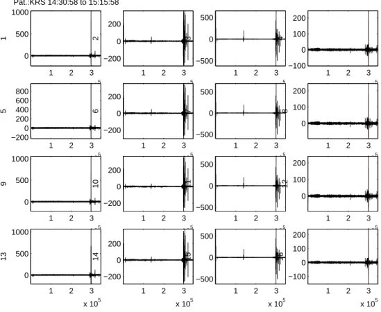
Twenty-two patients/seizures have been studied. From the application of the method, we could verify that for 13 patients k = 3 and for 9 patients k = 4. Fig.2 shows an example of the 16 EEG plots of a module-4 patient.
1 2 3
x 105 0
500 1000
1
Pat.:KRS 14:30:58 to 15:15:58
1 2 3
x 105 −200
0 200
2
1 2 3
x 105 −500
0 500
3
1 2 3
x 105 −100
0 100 200
4
1 2 3
x 105 −200 0 200 400 600 800 5
1 2 3
x 105 −200
0 200
6
1 2 3
x 105 −500
0 500
7
1 2 3
x 105 0
100 200
8
1 2 3
x 105 0
500 1000
9
1 2 3
x 105 −200
0 200
10
1 2 3
x 105 −500
0 500
11
1 2 3
x 105 0
100 200
12
1 2 3
x 105 0
500 1000
13
1 2 3
x 105 −200
0 200
14
1 2 3
x 105 −500
0 500
15
1 2 3
x 105 −100
0 100 200
16
Figure 2: EEG plots of module-4 patient (k = 4)
3. Classifying a patient/seizure as module-k allows for formally defining
linked channels.
For a patient module-4 the following pairs of channels are examples of
linked channels: [2,6],[2,10],[2,14] and [1,5],[5,9],[1,13].
Although linked channels seem to display synchronous behavior, when
the correlation coefficientsCij between pairs oflinked channels are com-pute, the resulting values do not show the existence of any stronger correlation, being the values of Cij close to those obtained for the cor-relation between any other pair.
However, when a time-delay is introduced between the linked
chan-nels, the similarity that is observed in their corresponding plots can be formally recognized. To this end, we proceed through the following steps.
4. For each pair of linked channels si and sj compute the correlation
co-efficient Cθ(i, j) at multiple time delays (θ).
Cθ(i, j) = h
si.sjθi−hsii.hsjθi
hσi.σjθi (1)
θ = ∆t
128 ∆t= 0,1,2,3,4 (2)
5. It was empirically observed that, for each pair oflinked channelssi and sj, there is a typical value ofθthat maximizes the correlation coefficient
Cθ(i, j)
6. The typical values of θ can be computed from the difference between the order numbers of the linked channelssi and sj, as below (eq.3).
θ(i, j)max = (
∆t
128)
i−j
k ∆t = 0,1,2,3,4 (3)
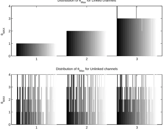
The first plot in Fig.3 shows the histograms of the values ofθthat maxi-mizes the correlation coefficients between three pairs oflinked channels.
The second plot shows the same results obtained for three pairs of un-linked channels.
1 2 3 0
1 2 3 4
Distribution of θ
Max for Linked channels
θ MAX
1 2 3
0 1 2 3 4
Distribution of θ
Max for Unlinked channels
θ MAX
Figure 3: Histograms of the values of θmax for 3 pairs of linked and for 3
pairs of unlinked channels (bottom)
Few minutes before the EEG seizure initiation the characteristic time delays remain almost unchanged for thelinked pairs, while some un-linked pairs display interesting changes in their typical time delays.
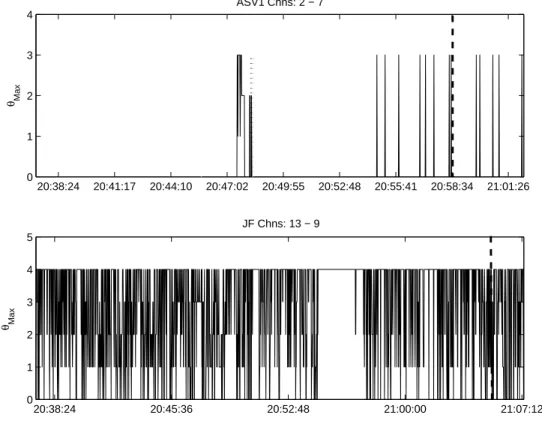
The plots in Fig.4 show the values of θmax varying in time for a pair of linked channels (top) and for unlinked pairs (bottom). The vertical
lines at time 12:28:48 indicate the occurrence of a seizure.
Althoughunlinked pairs display a much less uniform behavior in what
12:00:000 12:07:12 12:14:24 12:21:36 12:28:48 12:36:00 1
2 3 4 5
θ
Max
12:00:000 12:07:12 12:14:24 12:21:36 12:28:48 12:36:00 1
2 3 4 5
θ
Max
Figure 4: Values of θmax varying in time for linked and unlinked channels
(bottom)
as a crisis approaches. The dashed vertical lines indicate the occurrence of a seizure.
In both cases, the changes in the values ofθmax occur 10 to 15 minutes before the beginning of crises. In the first plot the (null) value of
20:38:24 20:41:17 20:44:10 20:47:02 20:49:55 20:52:48 20:55:41 20:58:34 21:01:26 0
1 2 3 4
ASV1 Chns: 2 − 7
θ Max
20:38:24 20:45:36 20:52:48 21:00:00 21:07:12
0 1 2 3 4 5
JF Chns: 13 − 9
θMax
Figure 5: Values of θmax varying in time for linked and unlinked channels
(bottom)
4
Questions
The work presented in this working paper raised some basic questions.
1. Why are there patients module-3 and patients module-4 ?
2. Where do those patterns come from?
3. Why are they (empirically) restricted to the values three and four ?
4. Why are they persistent in both monopolar and bipolar montages?
Future developments shall provide suitable answers to the above ques-tions. Finally, the predictive character of our approach is also to be explored in future work.