Fully non-invasive pressure drop measurements and post treatment prediction in congenital heart diseases via cardiac magnetic resonance and computer flow dynamics

(1)

UNIVERSIDADE DE LISBOA

FACULDADE DE CIÊNCIAS

DEPARTAMENTO DE FÍSICA

Fully non-invasive pressure drop measurements and

post treatment prediction in congenital heart diseases

via cardiac magnetic resonance and computer flow

dynamics

Rita Dias Cabrita Alves

Mestrado Integrado em Engenharia Biomédica e Biofísica

Perfil em Sinais e Imagens Médicas

Dissertação orientada por:

Prof. Nuno Matela, FCUL

Joao Fernandes, DHZB

(2)

(3)

I

Resumo

De acordo com os dados de 2017 da Organização Mundial da Saúde, as doenças cardiovasculares são a principal causa de morte a nível mundial. Se estes tipos de doenças não forem diagnosticadas e tratados atempadamente, podem levar a insuficiências cardíacas ou outras complicações irreversíveis.

As duas doenças cardiovasculares congénitas estudadas neste trabalho são a coarctação aórtica (CoA), caracterizada por uma estenose, habitualmente, na zona do arco da artéria aorta, e a doença da válvula aórtica (AvD), uma malformação ao nível da válvula aórtica. Estas doenças são responsáveis por cerca de 50,000 intervenções por ano. Deste modo, a melhoria métodos de diagnóstico e de intervenção adequados e eficientes é uma prioridade e pode levar ao decréscimo no número das intervenções, bem como reduzir a morbilidade e a mortalidade.

A área de imagiologia médica de diagnóstico tem tido uma evolução significativa ao longo dos anos e é de extrema importância nas tentativas de substituição de métodos de diagnóstico invasivos. As imagens médicas são adquiridas e posteriormente processadas e analisadas, com recurso a programas adequados. Atualmente, é possível obter os valores de gradientes de pressão relativa a partir de Ecocardiografia Doppler e Ressonância Magnética. Contudo, os gradientes de pressão medidos no cateterismo cardíaco, o método gold standard para o diagnóstico de CoA e AvD, são gradientes de pressão absoluta. Nesta dissertação desenvolveu-se um método de diagnóstico de CoA e AvD, a partir dos mapas de pressão relativa no estreitamento da aorta e na válvula aórtica, respectivamente.

O método matemático desenvolvido tem por base as equações de Poisson, resolvida com a condição de fronteira de Neumann utilizando os métodos de elementos finitos, e a de Navier Stokes para a conservação do momento. O método desenvolvido também tem em conta a informação proveniente da função de Windkessel da artéria aorta, uma artéria distensível. Esta função dá-nos o comportamento da propagação do pulso de pressão com uma velocidade de pulso de propagação. Deste modo, é observado um desfasamento temporal entre as curvas de fluxo da pressão e da velocidade, entre as duas regiões de interessante escolhidas. Deste modo, o método, denominado de Time-shift Corrected Pressure Maps (TCPM, sigla em inglês), permite obter os mapas de pressão absoluta, isto é, mapas de pressão que têm em conta o intervalo de tempo entre os picos de pressão na aorta descendente e ascendente, no caso do primeiro estudo, e antes e depois da válvula aórtica, no caso do segundo estudo. Os pacientes de ambos os estudos tinham indicação clínica para cateterismo cardíaco e foram submetidos a ressonância magnética cardiovascular de contraste de fase em tempo real (4D PC MRI, em inglês), para recolher as imagens ao nível da aorta e da válvula aórtica e os respectivos campos de velocidade da corrente sanguínea.

O primeiro estudo tem como objetivo a aplicação do método TCPM a 27 pacientes de CoA (n=16 masculinos, n=11 femininos, faixa etária de 4 a 52 anos, idade média de 20±15 anos). Após aquisição das imagens, estas foram processadas usando programas específicos. Em primeiro lugar foi necessário segmentar a aorta, seguiu-se a seleção das regiões de interesse e, finalmente, a obtenção dos campos de velocidade e dos mapas de pressão relativa entre as duas regiões de interesse selecionadas. Após aplicação do método TCPM, foram aplicados testes estatísticos (correlação, teste t e Bland-Altman) para comparar os valores obtidos a partir de TCPM com os valores obtidos no cateterismo cardíaco. Após processamento das imagens dos 27 pacientes, 6 pacientes foram retirados do estudo. N=3 pacientes foram retirados porque a percentagem de fluxo que passa pelo estreitamento é insuficiente para calcular o gradiente de pressão a partir de TCPM e N=3 pacientes foram retirados porque a aorta não estava inserida por completo no FOV. As medições obtidas a partir de TPCM e cateterismo cardíaco têm uma correlação linear significante (R²_{=0,90; p<0,001). A partir dos gráficos Bland-Altman é possível} verificar uma boa concordância entre as medições de ambos os métodos, com bias de -2,69 mmHg e os limites de concordância de

±4,74 mmHg

. O teste de equivalência mostrou uma relação significante entre os métodos (p=0,007).

(4)

II O segundo estudo tem como objetivo a aplicação do método TPCM e o método da Área de Gorlin a 4 pacientes de AvD (n=4 masculinos, faixa etária 17 a 36 anos, idade média 27±7 anos). O método da Área de Gorlin permite obter o gradiente de pressão absoluta a partir da área geométrica da válvula e do fluxo total que passa nessa área. Após a aquisição das imagens, foi feito o processamento das mesmas. Numa primeira fase, as imagens foram segmentadas na região da válvula aórtica. Depois, as imagens segmentadas foram analisadas em dois programas distintos. O primeiro foi utilizado de forma a obter os campos de velocidade e os mapas de pressão relativa entre dois pontos antes e depois da válvula aórtica. O segundo permitiu definir a região da válvula como região de interesse e exportar os valores de velocidade, área, pressão relativa e fluxo absoluto nessa região. Os resultados mostram uma correlação linear significativa entre os valores de cateterismo cardíaco e de TCPM (R²_{=0,99; p<0,001). Os gráficos} de Bland-Altman mostram uma boa concordância entre os valores de TCPM (24,75±22,50 mmHg) e de cateterismo (20,88±19,51 mmHg), com um bias de -3,87 mmHg e limites de concordância de ±3,64 mmHg. Os resultados também sugeriram uma ligeira subestimação dos valores do cateterismo cardíaco a partir do método da Área de Gorlin (14,47±13,00 mmHg), com um bias de 6,41 mmHg e limites de concordância de ±7,15 mmHg. Este estudo foi feito com uma amostra diminuta de 4 pacientes, o que não é suficiente para retirar conclusões com significância. Contudo, foi uma primeira abordagem positiva, que mostra a potencialidade que este método pode vir a apresentar.

O método TCPM proposto neste projeto permite a medição não invasiva de gradientes de pressão absoluta a partir de mapas de pressão relativa em pacientes de CoA e AvD. Vários aspectos têm que ser tidos em conta de forma a garantir a eficácia deste método. Por exemplo, as regiões de interesse escolhidas têm que se cuidadosamente selecionadas de forma a serem perpendicular à direção do fluxo naquele local. Só desta maneira é possível obter o fluxo, os campos de velocidade e as pressões relativas corretas. Também, se o raio da estenose for menor que 2 voxéis, a relação sinal-ruído aumenta substancialmente, e a resolução especial da aquisição é insuficiente. Contudo, a aplicação do método TPCM a casos de grande estreitamento não é necessária visto que estes casos já são tipicamente identificados em imagens anatómicas de ressonância magnética e que o paciente segue automaticamente para intervenção quando a área do estreitamente representa cerca de 50% do valor de área típico da aorta.

O método não invasivo TCPM apresenta uma boa concordância com o cateterismo cardíaco em termos da medição dos gradientes de pressão em CoA e AvD. Os bias e os limites de concordância entre cateterismo e TCPM foram substancialmente mais pequenos que os bias e os limites de concordância entre cateterismo e ecocardiografia Doppler e entre o cateterismo e o método da Área de Gorlin. Com os resultados apresentados já é possível ver o potencial desta técnica no processo de diagnóstico e decisão de intervenção em casos de CoA e AvD. Contudo, estudos com populações maiores será extremamente benéfico para validar clinicamente este método.

Palavras-Chave: Ressonância Magnética Cardiovascular, Coartação da Aorta, Gradientes de Pressão, Estenose Aórtica, Mapas de Pressão através de Ressonância Magnética, 4D PC-MRI.

(5)

III

Abstract

This dissertation aims to validate MRI-based time-shift corrected pressure mapping (TCPM) against cardiac catheterization in CoA and AvD patients. Also, in AvD patients, catheterization will be compared against Gorlin Area method. This project is divided in two independent studies: the first one for CoA patients and the second one for AvD patients, all with clinical indication for cardiac catheterization.

In both CoA and AvD, clinical guidelines recommend treatment in the presence of a relevant pressure gradient. While reliable non-invasive measurement approaches would be crucial, the accuracy of currently available methods has been limited.

In both studies, 4D PC-MRI was performed to compute relative pressure maps via Pressure-Poisson equation. To consider the patient-specific peak pressure time-shift from the ascending to the descending aorta and before and after the aortic valve, relative pressure gradient maps were corrected by the inertial term. Comparison between TCPM and invasive peak-to-peak measurements was performed using correlation, Bland-Altman plots and mean-equivalence t-test.

In the first study, with a cohort of 21 patients with CoA, TCPM and catheter measurements showed significant linear correlation (R²_{=0.90; p<0.001). Bland-Altman plots demonstrated good agreement} between TCPM and catheter derived pressure gradients with mean differences of -2.69 mmHg and 95% limits of agreement between -6.38 and 1.00 mmHg between methods. The mean-equivalence test was significant (p=0.007).

In the second study, with a cohort of 4 patients with AvD, the catheterization measurements were compared against TPCM measurements. The results showed significant linear correlation (R²_=0.99; p<0.001). Bland Altman plots showed a good agreement between TCPM (24.75±22.50 mmHg) and catheter derived peak-to-peak pressure gradients (20.88±19.51 mmHg), and suggested slight underestimation of the pressure gradients by the Gorlin Area method (14.47±13.00 mmHg).

Non-invasive TCPM showed equivalence to pressure gradients from invasive heart catheterization in patients with CoA and AvD. However, in the AvD study, they were obtained for a very small cohort of patients and do not have sufficient statistical significance to validate the method for AvD patients.

Key Words: Cardiac Magnetic Resonance Imaging, 4D PC-MRI, coarctation of aorta, pressure gradient; aortic valse disease; MRI pressure mapping;

(6)

IV

(7)

V

Acknowledgements

I would like to express my sincere gratitude to both my supervisors Prof. Nuno Matela and João Fernandes, for the support and patience throughout this whole year.

Thank you to all the team members from DHZB that accompanied me during the internship and that taught me things I will take with me for the rest of my life. João Fernandes, Tiago Silva and Alireza Khasheei, it was a pleasure to share the same workspace, to avoid dinner and to talk about the future with all of you (despite my morning mood).

To all the professors from the Institute of Biophysics and Biomedical Engineering my sincere thanks for all the knowledge you shared with me and my colleagues. You are the main reason why we all have such great opportunities and hope no one did disappoint you.

Without the constant support of my friends this thesis would not be a reality. To “Pessoal Fixolas” the biggest “Thank you!” of the world. You were responsible for keeping me happy and grounded while away from everything I knew. A special thanks to Tatiana Costa, Marta Carrilho, Filipe Costa and Tânia Gonçalves for enjoying Berlin with me, enduring the cold and the never-ending tour I prepared, for making me eat breakfast, for the snow fights and for the birthday I thought I could never have. To my favourite “Berliners”, Andreia, Christina, Iara, Julia, Katherine, Leonor, Patrick, Rita, Selin and Tobias, thank you for teaching me so much about your culture and for making Berlin feel like home.

My family was crucial for all of this. My parents were the biggest supporters of this whole adventure, not only this last year, but since I was born. Thank you for allowing me and Jorge to fly away but also for remind us where home is. My brother, the biggest example that inspires me every day to dream and to not be afraid of trying anything I set my mind into. And finally, my grandmothers, my personal heroes, that motivate me to work hard but enjoy life to the maximum. Your soup was missed in those 10 months I lived abroad.

This thesis is an accomplishment. And I am lucky that I have this great group of people surrounding me and celebrating with me this new phase of my life. Thank you! Obrigada! Vielen Dank!

(10)

(11)

IX

List of Figures

Figure 1 - Comparison between left ventricle and right ventricle in terms of shape and myocardium thickness in dilated and contracted moments [101]. ... 1 Figure 2 - Aorta and its division in three parts: ascending aorta, aorta arch and descending aorta. Adapted from [2]. ... 2 Figure 3 - Position of the aortic valve in between the left ventricle and the aorta. Schematic behavior of the aortic valve in the moments open and closed. [99] ... 2 Figure 4 – Left Ventricle and Aorta of a 10 years old patient with CoA. The narrowing is indicated with a red arrow. ... 3 Figure 5 - Comparison between a healthy valve and valves with Aortic Valve Disease. ... 3 Figure 6 - Spin Echo pulse sequence (a) and Gradient-echo pulse sequence (b). There are 5 events that compose the pulse sequence: radio frequency pulses (RF), readout gradient axis (Grd), phase-encode gradient axis (Gpe), slice-selection gradient axis (Gss) and acquired echoes (signal). ... 5 Figure 7 - Turbo Spin-Echo, Fast Spin-Echo or Rapid Acquisition with Relaxation Enhancement sequence. ... 6 Figure 8 - Spoiled Gradient-Recalled Echo Sequence (a) and Balanced Steady-State Free Precession Sequence (b). ... 6 Figure 9 - Data acquisition and analysis workflow for 4D flow MRI. (A) 4D flow MRI data covering the whole heart (white rectangle) is acquired using ECG gating. 3D velocity-encoding is used to obtain velocity-sensitive phase images which are subtracted from a reference image, in order to calculate blood flow velocities along all three spatial dimensions (Vx, Vy, Vz). (B) Data preprocessing corrects for errors due to noise, aliasing and eddy currents. Then the 3D phase-contrast-MRI is calculated. (C) 3D Blood flow is visualized by emitting time resolved pathlines from analysis planes in the Aorta, Inferior Vena Cava and Superior Vena Cava. In addition, retrospective quantitative analysis can be used to derive flow-time curves at user selected regions of interest in the cardiovascular system [101]. ... 7 Figure 10 - Origin of the wrap-around artifact. Two regions (R and L) are both mismapped at different phases, and these redudant phases are foldedback into the range of acquisition.[100] ... 8 Figure 11 – (A) Effect of vertical height on pressure in a frictionless fluid flowing downhill. (B) Effect of increasing cross-sectional area on pressure in a frictionless fluid system. Adapted from [3]. ... 10 Figure 12 - Example curves derived from Poiseuille's Law. There are three curves of the pressure gradient behavior with the increase of area of stenosis for different volume flows: 50 cm3_{/s (red),}

10cm3_{/s (blue) and 5 cm}3_{/s (green) [1]. ... 11} Figure 13 – The Windkessel effect can be compared to the air chamber used in fire engines. The Windkessel effect helps in alleviate the fluctuation in blood pressure over the cardiac cycle and assists in the maintenance of organ perfusion during diastole when cardiac ejection ceases. ... 17 Figure 14 - Block diagram that illustrates the method follow and summarizes the equations used (1) Flow distribution in the ascending (blue) and descending (red) aorta. A and B are the time steps in which there is a peak flow in the ascending and descending aorta, respectively. (2) Relative pressure

(12)

X distribution / field / map of the aorta during systole. There are two planes, one in the ascending aorta and other in the descending aorta. dx is the distance between two planes. ... 18 Figure 15 - Bland Altman analysis to compare catheterization and MRI TCPM. The bias is -2.59 mmHg and the limit is ±4.74 mmHg. ... 20 Figure 16 - Scatterplot of the measurements from catheterization and MRI in mmHg. The red line is the trend line of the linear correlation between the two methods. The correlation coefficient between both absolute measures (catheter and MRI) is 0.88. The correlation equation is CMR =0.94Catheterization + 3.93 ... 21

Figure 17 - Flow through a stenotic aortic valve. AAo indicates ascending aorta; EOA, effective orifice area; GOA, geometric orifice area; LVOT, left ventricular outflow tract; VC, vena contracta; VTl, velocity time integral [26]. ... 26 Figure 18 – Aortic Valve mask with the regions of interest and the Start, End and Reference points chosen. It is considered the aortic valve as the reference point. ... 30 Figure 19 - Bland Altman analysis to compare catheterization and time shift corrected pressure gradients in patients with AS. The bias is -3.87 mmHg and the limit of agreement is ±7.13 mmHg. ... 31 Figure 20 - Bland Altman analysis to compare catheterization and Gorlin Area method pressure gradients, in patients with AS. The bias is 6.41 mmHg and the limit of agreement is ±7.15 mmHg. .. 32 Figure 21 - Scatterplot of the measurements from catheterization and time shift corrected pressure gradients in mmHg, in patients with AS. The red line is the trend line of the linear correlation between the two methods. The correlation coefficient between both absolute measures (catheter and MRI) is 0.99. The correlation equation is CMR = 1.15Catheterization + 0.79 ... 32 Figure 22 - Scatterplot of the measurements from catheterization and Gorlin Area method pressure gradients, in mmHg, in patients with AS The red line is the trend line of the linear correlation between the two methods. The correlation coefficient between both absolute measures (catheter and MRI) is 0.97. The correlation equation is CMR = 0.65Catheterization+0.80... 33

(13)

XI

List of Tables

Table 1 - Recommendations for classification of Aortic Valve Stenosis severity according to European Society of Cardiology [24].

... 4

Table 2 - Quantitative parameters for Aortic Valve Regurgitation classification according to European Society of Cardiology [6].

... 4

Table 3 - Patients characteristics and values of absolute and relative pressure gradients obtained via catheter and MRI.

... 19

Table 4 - Patients characteristics and values of absolute and relative pressure gradients obtained via catheter and MRI.

... 31

(14)

XII

(15)

XIII

List of Abbreviations

AV – Aortic Valve

AvD – Aortic Valve Disease

AVR – Aortic Valve Regurgitation

AVS – Aortic Valve Stenosis

CHD – Congenital Heart Diseases

CoA – Coarctation of the Aorta

CT – Computer Tomography

FA – Flip Angle

FOV – Field of View

LA – Left Atrium

LV – Left Ventricle

MRI – Magnetic Resonance Imaging

PC – Phase Contrast

ROI – Region of Interest

RV – Right Ventricle

SE – Spin-Echo

TE – Echo Time

TOST – Two One-Sided Test

TR – Repetition Time

VC – Vena Contracta

(16)

XIV

(17)

XV

Motivation

According to the World Health Organization, cardiovascular diseases (CVDs) are the principal cause of death globally. CVDs are a group of disorders of the heart and blood vessels and can lead to irreversible heart complications [1]. Congenital Heart Diseases are diseases that occur when the heart and the blood vessels near the heart do not develop normally before birth. In this dissertation, the two diseases discussed are coarctation of the aorta (CoA) and aortic valve disease (AvD). Catheterization is the gold standard for diagnosis and intervention, for both diseases. Catheterization is an invasive procedure that could lead to: bleeding, infection and bruising at the catheter insertion site; blood clots, which may trigger a heart attack; damage to the artery where the catheter was inserted, or damage the arteries as the catheter travels through the body. To provide adequate prognosis and treatment and avoid the need of an invasive examination to detect these diseases, it is necessary an approach to improve diagnosis.

While non-invasive diagnostic methods would be preferable, cardiac catheterization is still seen as the clinical reference standard for CoA and AvD evaluation at many centres. However, current noninvasive methods are unsatisfactory, since they are highly inaccurate [1, 2]. For example, cuff based measurements provide pressure differences between peripheral arteries and are affected by anatomic variation, pulse wave velocities, measurement setting and cuff-size [2,3]. Doppler echocardiography applies a simplified Bernoulli equation, which tends to overestimate the pressure gradient, since maximal velocities across the stenosis are increased due to higher wall stiffness and presumes the presence of an ideal fluid [4, 5].

Four-dimensional velocity encoded MRI (4D-VEC MRI) was shown to be able to map the relative pressures in one vessel [6]. Although relative pressure maps do not take into account the time shift parameter that invasive peak-to-peak measurements take, manual corrections, by adding single cuff measurements and a standard pressure curve, have been suggested [7].

The aim of this dissertation is to demonstrate a novel method of non-invasive MRI-based time-shift corrected pressure mapping to assess pressure gradients and to validate it against peak-to-peak pressure differences obtained from invasive heart catheterization. This method will also be compared against other commonly used non-invasive measurements, such as measurements based on cuff pressures and

(18)

XVI

(19)

1

1. Background Material

1.1. Cardiovascular Structures of Interest

1.1.1. Left Ventricle

The Left Ventricle (LV) is the structure that receives blood from the Left Atrium (LA) and pumps it to all the tissues of the body, through the aorta. Most of the left lateral surface of the heart is formed by the LV. Also, it forms part of the inferior and posterior surfaces. The wall of the LV is characterized by trabeculae carneae (also referred as “beams of meat”) which are rounded or irregular muscular columns. Comparing the LV to the Right Ventricle (RV), the muscular columns tend to be relatively thinner and the myocardium in the wall of the LV is much thicker (Figure 1) [8].

1.1.2. Aorta

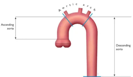
The aorta is the largest artery in the body. It can be divided in three main sections: the ascending aorta, which supplies the arms and head, the descending aorta, which supplies the lower part of the body, and the aortic arch that connects the ascending section to the descending section. The aortic arch has an inverted U form and is the origin of three major arteries: left subclavian artery, left common carotid artery and brachiocephalic artery (Figure 2) [2]. The aorta is of absolute importance since every major organ, except the liver, is supplied by arteries that arise from the aorta [9].

Since the structure of the aorta contains a high density of elastic fibers, it can tolerate the pressure changes characteristic of the cardiac cycle. During LV systole, pressures rise rapidly and aorta expands. When the pressure drops in LV diastole, the elastic fibers recoil to their original dimensions. This recoil slows the pressure drop in the adjacent vessels during LV diastole. Therefore, the wall characteristics of the elastic arteries are the main reason for the absence of pressure oscillations when the blood reaches the arterioles in healthy subjects.

Figure 1-Comparison between left ventricle and right ventricle in terms of shape and myocardium thickness indilated and contracted moments [101].

(20)

2

1.1.3. Aortic Valve

The aortic valve (AV) is one of the semilunar valves of the heart. Semilunar refers to the shape of the valve cups visible in a frontal section of the heart. The AV is the site where the aorta joins the LV (Figure 3). This valve is responsible for the controlled blood flow from the LV to the aorta. It is compose by three leaflets, although approximately 2% of the population has congenitally two leaflets [10].

1.2. Cardiovascular Diseases of Interest

1.2.1. Coarctation of the Aorta

CoA is a narrowing of the aorta and is one of the most common diseases in the aorta, accounting for 5-8% of all congenital heart diseases (CHD) (Figure 4) [11]. Due to its location, CoA can have different definitions: if it is located less than 10mm from the origin of the left subclavian artery it is defined as proximal CoA; if it is located more than 10mm from the origin of the left subclavian artery it is defined as distal CoA [12].

CoA has clinical features that include upper body systolic hypertension and lower body hypotension, creating a blood pressure gradient between upper and lower extremities. The blood pressure gradient is the main diagnostic factor for CoA [13].

Figure 2-Aorta and its division in three parts: ascending aorta, aorta arch and descending aorta. Adapted from [2].

Figure 3- Position of the aortic valve in between the left ventricle and the aorta. Schematic behavior of the aortic valve in the moments open and closed. [99]

(21)

3

This disease can be mild or severe. It is considered that a CoA is severe if the pressure gradient across the narrowing is equal or higher than 20 mmHg and mild if the pressure gradient is less than 20 mmHg. In cases of severe CoA the patient is submitted to surgery. There are various surgery options such as stents and balloon angioplasty [14].

1.2.2. Aortic Valve Disease

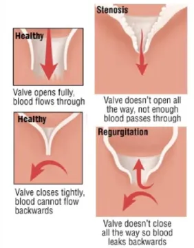
AvD is one of the most common and most serious valve disease problems. There are two main types of aortic valve disease: Aortic Valve Stenosis, when the AV opening is narrowed, which prevents it from opening fully and obstructs blood flow, and Aortic Valve Regurgitation, when the AV does not close properly, which allows blood to flow backward into the LV. It can occur because of calcification and congenital valvular defects such as bicuspid AVs or rheumatic disease (Figure 5) [15].

Figure 4–Left Ventricleand Aorta of a 10 years old patient with CoA. The narrowing is indicated with a red arrow.

Figure 5-Comparison between a healthy valve and valves with Aortic Valve Disease.

(22)

4

Due to the modified blood flow in and out of the heart, the LV needs to work more intensively to pump the blood through the AV. This can lead to a remodel of the shape of the LV and may also affect the pressure in the LA [16].

Aortic Valve Stenosis (AVS) and Aortic Valve Regurgitation (AVR) can be characterized based on their severity. The clinical guidelines to characterize each disease are present in the following tables 1 and 2:

Table 1 - Recommendations for classification of Aortic Valve Stenosis severity according to European Society of

Cardiology [24].

Mild Moderate Severe

Aortic Jet Velocity (m/s) 2.6 – 2.9 3.0-4.0 >4.0

Mean Gradient (mmHg) <30 30-40 >40

Aortic Valve Area (cm2) >0.85 0.60-0.85 <0.6

Velocity ratio (cm2/m2 >0.50 0.25-0.50 <0.25

Table 2 - Quantitative parameters for Aortic Valve Regurgitation classification according to European Society of

Cardiology [6].

Mild Moderate Severe

Regurgitant Volume

(mL/beat) <30 30-59 ³60

Regurgitant Fraction (%) <30 30-49 ³50

Effective Regurgitant Orifice >0.85 0.10-0.29 ³0.30

For AVR patients, intervention is recommended when ejection fraction ≤50% and when there is LV enlargement with an LV end-diastolic diameter (LVEDD) >70 mm or left ventricular endsystolic diameter (LVESD) >50 mm. For patients close to these intervention thresholds, it is advised close follow. In asymptomatic patients, regular assessment of LV function and physical condition are crucial to identify the optimal time for surgery. A rapid progression of ventricular dimensions or decline in ventricular function on serial testing is a reason to consider surgery [17].

For AVS patients, intervention is recommended for patients with severe AVS and DP ≥ 40 mmHg. The only exceptions are patients with severe comorbidities indicating a survival of less than a year and patients whom would be unlikely to get an improved quality of life from the

intervention. Initial diagnosis of AVS typically is obtained during routine physical examination

with the presence of a heart murmur or other abnormal sounds. Undiagnosed subjects can experience severe symptoms like angina or heart failure [18].

1.3. Basic Principles of Cardiac Magnetic Resonance Imaging

Cardiac Magnetic Resonance (MRI) is the Magnetic Resonance Imaging when applied to the heart and main blood vessels and uses Magnetic Resonance sequences optimized for the

(23)

5

cardiovascular system. It is a well-established method to analyze the anatomy and pathophysiology of the cardiovascular system, and therefore is also an alternative method of diagnosis and decision making on cardiovascular diseases.

One of the biggest technical challenges that MRI must overcome is the rapid and complex motion of the heart. Also, effects of respiratory motion and systolic ventricular blood velocities (that can reach 500cm/s in certain pathologies) have to be taken into account [19]. To generate images free of motion artifacts, the images are acquired quickly, using or improved scanners, that allow faster gradients, or rapid imaging techniques, such as parallel imaging [20]. Furthermore, breathhold techniques are also used.Typical MRI parameters are: field of view (FOV) 350 x 350 𝑚𝑚2_{, repetition time (TR) = 2.8 ms, echo time (TE) = 1.4 ms, acquired voxel size = 2.2} x 2.2 x 8 mm3_{, flip angle (FA) = 60ºand reconstructed voxel size = 1.3 x 1.2 x 8 mm}3_.

The orientation of the heart within the chest varies from patient to patient and this variable makes the localization of the images unpredictable. Most of the cardiac imaging techniques use cardiac axes, which need to be identified for each individual patient. A full-chest sequence is necessary as localizer and after these, various sequences are planned such as transverse, sagittal and coronal.

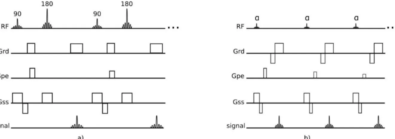
Pulse sequences are programed to encode the timing and magnitude of the pulses emitted by the MR. Spin-echo (SE) and gradient-echo pulse sequences are very relevant in MRI. A SE pulse is produced by pairs of radiofrequency (RF) pulses, whereas gradient-echo pulse is produced by a single radiofrequency pulse in conjunction with a gradient reversal (Figure 6).

1.3.1. Spin-Echo Sequences

Spin-Echo sequences offer a bigger ability in obtaining different contrasts depending on the choice of TE and TR. These different contrasts can be T1-weighted, T2-weighted or proton density-weighted. SE sequences refocus the excited signal with a 180° pulse (or pulses) and this makes the signal less vulnerable to off-resonance effects that can be caused by main field inhomogeneities or magnetic susceptibilities.

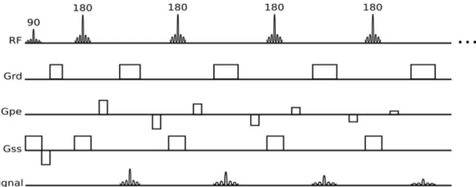
The main disadvantages of this type of sequences are their sensitivity to motion and flow and their limited temporal-resolution. There is also the option to shorten the SE sequences acquisition times and, in this situation, the SE pulse sequence becomes turbo SE, fast SE or rapid acquisition with relaxation enhancement. The acquisition times are shortened using a multi-echo approach in which multiple refocused echoes are acquired preceded by a single 90° excitation pulse (Figure 7). The reduction of acquisition time allows the acquisition of a whole image within a breath-hold, reducing the artifacts that could occur from breathing motion.

Figure 6-Spin Echo pulse sequence (a) and Gradient -echo pulse sequence (b). There are 5 events that compose the pulse sequence: radio frequency pulses (RF), readout gradient axis (Grd), phase-encode gradient axis (Gpe), slice-selection gradient axis (Gss) andacquired echoes (signal).

(24)

6

1.3.2. Gradient-Echo Sequences

Unlike SE sequences, gradient-echo sequences do not have refocusing pulse. This makes the signal more susceptible to off-resonance effects, which makes this class of sequences generally T2* weighted instead of T2, thus because of the faster signal decay there is a need for shorter TE.

Gradient-Echo sequences allow faster image acquisition than SE sequences, which is an advantage for MRI characterization of the cardiac cycle. This rapid acquisition does not allow either the longitudinal or transverse magnetization to fully relax between successive radiofrequency pulses. The magnetization achieves an equilibrium state, known as steady state during the multiple excitations of the sequence. There are two strategies that can be employed to deal with the remaining magnetization at the end of each TR: the remaining transverse magnetization can be spoiled in Gradient-Recalled-Echo sequence (Figure 8a) or it can be refocused and reused as in the balanced steady–state free precession sequence (Figure 8b). Using this sequence is possible to obtain cine imaging. Cine sequences consist of a group of images at the same spatial location covering one full period of the cardiac cycle.

1.3.3.

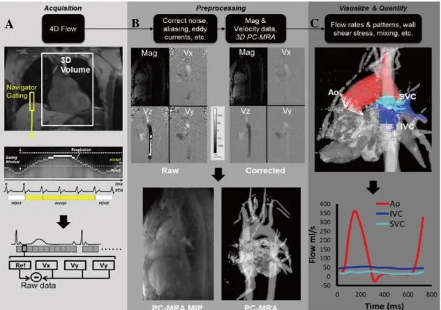
4D Phase Contrast Imaging

Phase Contrast (PC) imaging allows quantitative blood velocity information. Combining this sequence with the ability of mapping the cardiac cycle via cine imaging to produce images

Figure 7 - Turbo Spin-Echo, Fast Spin -Echo or Rapid Acquisition with Relaxation Enhancement sequence.

(25)

7

throughout the time, it is possible to visualize and quantify blood flow velocity within the heart or vascular regions of interest in 3D and over time (4D) (Figure 9).

The applications of gradient pulses induce phase shifts in moving protons that are directly proportional to their velocity along the direction of the gradient. For accurate quantification of this phase shift, a reference image is acquired separately to subtract phase shifts induced by other uncontrollable factors, such as magnetic field inhomogeneities. From repeating the acquisition for 3 orthogonal directions, it is possible to obtain phase maps which encode velocity (𝑉H, 𝑉I, 𝑉J) to a maximum velocity defined by the user (VENC). VENC stands for velocity encoding and should be chosen to enclose the highest velocities likely to be encountered within the vessel of interest. The VENC parameter adjusts the bipolar gradients. This means that, the maximum velocity selected corresponds to a 180° phase shift in the data. Thus, for each pixel, the measured phase depends on the velocity of the spins. Thus, stationary protons appear grey, spins that flow in the direction of the gradients appear brighter, and spins that move in the opposite direction appear darker. This is visible by an inverted signal where the intensity signal has a maximum brightness correspondent to phase shifts that overcome ±180°. Given this, the

C

B

A

Figure 9-Data acquisition and analysis workflow for 4D flow MRI. (A) 4D flow MRI data covering the whole heart (white rectangle) is acquired using ECG gating. 3D velocity-encoding is used to obtain velocity -sensitive phase images which are subtracted from a reference image, in order to calculate blood flow velocities along all three spatial dimensions (Vx, Vy, Vz). (B) Data preprocessing corrects for errors due to noise, aliasing and eddy currents. Then the 3D phase-contrast-MRIis calculated. (C) 3D Blood flow is visualized by emitting time resolved pathlines from analysis planes in the Aorta, Inferior Vena Cava and Superior Vena Cava. In addition, retrospective quantitative analysis can be used to derive flow-time curves at user selected regions of interest in the cardiovascular system [101].

(26)

8

velocity, v, within each voxel can be determined by the mean of the protons phase difference, ΔΦ, accrued during one time step (temporal resolution), using the formula:

_{ΔΦ =γΔmv (1.1)}

where γ is the gyromagnetic ratio and Δm denotes the difference of the first moment of the gradient-time curve. On the other side, a too high VENC for the selected region will induce significant levels of noise.

The closer the VENC is to the maximum expected velocity (ideal VENC), the more precise is the measurement. If the VENC selected is lower than the velocity within the vessel, aliasing or phase wrapping occurs. However, a VENC setting of three times the ideal value (on low velocity regions) is considered to be an acceptable value [21]. There are clinical guidelines for VENC determination such as 100, 200, 400 cm/s for normal tricuspid valve, healthy aorta and tricuspid valve stenosis, respectively [22].

Sources of errors in PC-MRI acquisitions include inadequate VENC values, deviation of the imaging plane during data acquisition (e.g., cardiac, respiratory bad gating or patient motion), inadequate temporal or spatial resolution, and field inhomogeneity (e.g., susceptibility artefact from metallic implants). Therefore, depending on the structure of interest, PC-MRI parameters should be set in order to minimize potential sources of error [23].

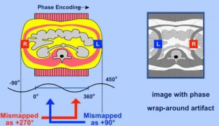
1.3.4.

Phase Wrapping

As described in the previous subsection, phase is a parameter of interest for the measurement and analysis of the blood flow. If the value of phase extends beyond 360 degrees or, in other words, if the dimensions of an object exceed the defined field-of-view, the redundant phase will be folded back into this range, leading to ambiguity in the final phase. This will induce an artifact in the image called phase wrap-around. The wrap-around artifact is generally recognized as a folding over of anatomic parts into the area of interest. (Figure 10) [24].

Figure 10-Origin of the wrap-around artifact. Two regions (R and L) are both mismapped at different phases, and these redudant phases are foldedback into the range of acquisition.[100]

(27)

9

2. Fluid Mechanics applied to blood vessels

To develop a mathematical method to obtain absolute pressure gradients in both aorta and AV, it is necessary to understand their hemodynamic performance and the physical laws that govern their function.

2.1. Principle of Conservation of the mass

The principle of conservation of mass is a mass balance over a certain control volume. This volume can coincide with a section of an artery, with the LV or even with the surface of a blood cell. The boundaries of the control volume are usually chosen to give information regarding unknown flow rate, average velocity or surface area flow into or out of the volume [25].

The density of blood is constant, and since mass is the product of density and volume, mass conservation can be expressed as volume conservation for cardiovascular applications. The equation that expresses follows:

in which 𝑄UV is the total flow rate into the control volume, 𝑄WXS is the total flow rate out of the control volume, 𝑉U is the size of the control volume at the beginning of the observation, and 𝑉Y is the size of control volume after an observation time 𝑡. This equation is true for control volume that change with time, such as the volume of the LV. However, for most blood vessels, is possible to consider that the volume does not change with time. In these cases, the left side of equation 2.1. is zero, and conservation of the mass can be expressed as:

Flow rate in circular and nonbranching vessels can be decomposed into an average velocity 𝑣 and a cross sectional area (CSA). In this case conservation of the mass can define unknown average velocities or CSAs into or out of the control volume:

2.2. Mechanical Energy and Bernoulli’s equation

Mechanical energy can be described as the capability to accelerate a mass of material over a distance. There are three forms of mechanical energy per unit volume in the circulation: pressure, gravitational and kinetic energy. Even though pressure is the primary form of mechanical energy per unit volume in the healthy arterial circulation, in cases of diseased or venous circulations, gravity and kinetic energy play a significant role in the movement of flow [26].

Pressure (𝑃) represents a force (𝐹p) per unit area. If this force is responsible for moving a mass (𝑚) over a distance (𝑑), it performs work, expending pressure energy (𝐸_). The area where the force acts on multiplied by the distance represents a volume (𝑉):

(28)

10

A mass (𝑚) accelerating due to gravity (𝑔) creates a force (𝐹g). If this force moves the mass over a vertical distance (ℎ), it too performs work and expends gravitational energy (𝐸g). The energy per unit volume is obtained by substituting density (𝜌) for mass per unit volume:

If a mass (𝑚) is moving at a velocity (𝑣), it contains kinetic energy, equivalent to half the product of mass and the square of the velocity of the mass:

All the mechanical energy per unit volume forms can be freely converted from one to another without energy loss. Bernoulli’s equation for steady flow relates the relative amounts of pressure, gravitational and kinetic energy per unit volume between two spatial locations along a path of a flow (locations 1 and 2, where 2 is downstream of location 1):

Bernoulli’s equation for steady flow states the total mechanical energy per unit volume at locations 1 and 2 is the same but can exist in different forms. It shows that a decrease in pressure from location 1 to location 2 may be balanced from an increase in either fluid velocity or height without loss of energy. A pressure drop is therefore not mechanical energy loss if it is accompanied by increases in either gravitational or kinetic energy [26].

Two examples are illustrated in Figure 11. As a first example, blood enters the top of an inclined tube with a pressure of 100 mmHg and flows out at a pressure of 178 mmHg. The fluid moves against a pressure gradient from a point of low pressure (the beginning of the tube) to a point where the pressure is higher (end of the tube). However, the total fluid energy remains constant because the gravitational energy decreases is equal to the increase in pressure. This is what occurs in the arteries of a standing person (Figure 11A). As a second example, blood flows through a horizontal tube while the cross-sectional area increases 16 times. This results in a proportional decrease in fluid velocity. Again, the fluid moves against a pressure gradient, the pressure at the exit of the tube being 2.5 mm Hg greater than the pressure at the entrance to the tube. The total fluid energy remains the same because of the decrease in kinetic energy. This phenomenon is rarely observed in the human circulation because associated energy losses effectively mask the slight rise in pressure. (Figure 11B) [26].

(29)

11

To account for the effects of unsteady flow and mechanical energy loss, additional variables can be added to Bernoulli’s equation for steady flow:

where s represents the distance of the path between locations 1 and 2 and Φ represents loss of mechanical energy per unit volume. The two added terms represent the contribution of temporal acceleration of the fluid to the flow energy and the conversion of mechanical energy to heat, respectively, between locations 1 and 2 [26].

2.3. Poiseuille’s law

The specifications of the Bernoulli equation are theoretical and non-possible to achieve in human circulation. Mechanical energy can be lost in the movement of blood or fluid from one point to another (and normally is converted to heat). Energy loss is related to the viscosity of blood and its inertia. In fluids, viscosity can be defined as the friction between adjoining layers of fluid. This friction is due to strong intermolecular attractions between fluid layers. Poiseuille’s law describes the viscous energy losses occurring in an idealized situation [26].

in which 𝑃q − 𝑃F is the pressure drop between two points separated by the distance 𝐿, 𝑄 is the volume flow, and 𝑉 is the mean flow velocity across a tube with an inside radius of r. From Equation 2.9 is possible to establish that energy losses are inversely proportional to the fourth power of the radius. Figure 12 illustrates the Poiseuille’s Law in different cases. It shows that, until a certain degree of narrowing is reached, there is little effect on the pressure. Beyond that point, further reductions in diameter cause the pressure gradient to rise rapidly. Although increasing the flow rate shifts the curves to the left and linearly increases the pressure gradient at any given radius, these effects are much less marked than those caused by changes in radius.

(30)

12

2.4. Energy Losses associated with stenosis

Most of the abnormal energy losses in the arterial system result from stenosis or obstruction of the vascular lumen. In accordance with Poiseuille’s law (Equation 3.9), the energy losses are inversely proportional to the fourth power of the radius at the stenosis and are directly proportional to the length of the stenosis. Therefore, the radius of a stenosis is much more significant than its length [26]. In addition, inertial energy losses are encountered at both the entrance to and the exit from a stenosis [27, 28]. The magnitude of these losses varies with the shape of the entrance and exit. The energy losses associated with asymmetrical stenosis exceed those associated with symmetrical stenosis, even when the lumen is compromised to the same extent [28, 29]. Although energy losses at the entrance can be appreciable, they are usually greater at the exit, where much of the excess kinetic energy resulting from the increased fluid velocity within the stenosis is dissipated in a turbulent jet.

Experimentally, appreciable changes in pressure and flow do not occur until the cross-sectional area of a vessel has been reduced by more than 75% [30]. The degree of narrowing at which pressure and flow begin to be affected has been called the “critical stenosis.”

Energy losses across stenotic segments also depend on the velocity of blood flow (as shown in equation 3.8). Significant drops in pressure and flow occur with less severe narrowing in high-flow systems than in low-flow systems [31].

Precise attempts to relate pressure and flow restriction to percentage stenosis have been frustrated by the irregular geometry of arterial lesions and by the nonlinearities introduced by pulsatile blood flow. For practical purposes, any lesion that potentially decreases the arterial lumen by about 75% cross-sectional area or 50% diameter must be suspect, and its hemodynamic significance must be determined by objective physiologic tests.

The method proposed in this thesis attempts to calculate the peak-to-peak pressure drop using flow rate, velocities and relative pressure measurements obtained via MRI, in both patients of CoA and AvD. Both studies were approved by institutional research ethics committee following the ethical guidelines of the 1975 Declaration of Helsinki. Written consent was obtained from the participants and/or their guardians.

(31)

13

3. Materials

3.1. Catheterization

Routine catheterization procedures aiming to make a final treatment decision were performed under monitoring with a Philips Allura Xper FD 10/10 biplane angiography system (Philips Medical Systems, Best, The Netherlands), using contrast agent injection (Ultravist, Schering, Berlin, Germany). The pressure curves were recorded (Schwarzer Haemodynamic Analysing System, Heilsbronn, Germany) in two predefined locations via catheter pull back. Peak-to-peak pressure gradients across CoA and AvD were obtained from these pressure curves and used to validate MRI based pressure mapping.

3.2. Doppler Echocardiography

Diagnostic echocardiography was performed from the jugular fossa using a 3.5 MHz transducer interfaced with a Vivid E9 and processed with EchoPAC (GE Healthcare, Chicago, Il, USA). The continuous wave Doppler beam was aligned with the narrowing region to detect the maximum velocity Vmax through the CoA. The pressure gradient is obtained via the simplified Bernoulli equation:

3.3. MRI equipment and protocol

MRI was conducted, before catheterization, in a 1.5 T magnetic resonance scanner (Achieva R 3.2.2.0, Philips Medical Systems, Best, the Netherlands) using a 5-element cardiac phased-array coil (Philips Medical Systems). Three directional blood flow velocities (vx, vy, vz) were measured over the cardiac cycle using anisotropic k-space segmented 4 directions velocity encoded MRI (4DVEC-MRI) with electrocardiographic gating. The acquisition covered the full LV and the thoracic Aorta (ascending, arch and descending). Exemplary 4D-VEC-MRI scan parameters were: FOV feet-to-head 180 mm; anterior-to-posterior 200 to 230 mm (depending on size of the patient); rightto-left 90 to 105 mm (depending on number of slices and slice thickness); acquired voxel 2.5 × 2.5 × 2.5 mm; reconstruction matrix 128 × 128; reconstructed voxel 1.7 × 1.7 × 2.5 mm; flip angle of 5°; shortest TR and TE; nominal temporal resolution varying with heart rate for 25 cardiac phases; and velocity encoding 400 cm/s. Scan time varied between 8.5 and 14 min, depending on the chest size of the patient. 3D anatomy MRI was acquired at end-diastole. The typical scan parameters were: acquisition matrix 100x100; voxel size 1.2×1.2×2.0mm; repetition time 3.6ms; echo time 1.8ms. Acquisition duration was typically 2 min.

3.4. Post Processing Software

3.4.1.

MevisFlow

Although non-invasive measurements of patient 4D hemodynamics have been facilitated by the innovation of MRI techniques, the high number of processing steps and data complexity mean that data analysis remains challenging. MevisFlow software (Fraunhofer MEVIS, Bremen, Germany) introduced new processing and visualization approaches for 4D PC-MRI data. Some

(32)

14

features included in the software are 3D flow visualization, velocity vector field quantification and color coding of local hemodynamic according to, for example, local velocity or pressure. In the context of this work, this program was used in both CoA and AvD studies to: perform semi-automatic watershed 3D segmentation of the lumen and create the mask of the aorta and AV region; determine the blood velocity and flow patterns in the mask; calculate and visualize the relative pressure maps. This is accomplished by using particle tracing based on the magnitude and three directional field images together with the previously segmented aorta.

3.4.2. GTFlow

GTFlow (GyroTools LLC, Winterthur, Switzerland) is a software that delivers all the necessary functionality for visualization, assessment and interpretation of multidimensional MRI phase-contrast flow datasets. In opposite to MevisFlow, it allows the creating of new visualization planes, perpendicular to the MRI sequences. This software was only used for the

AvD study, to create a plane in the valve area and obtain the hemodynamic values in that region.

(33)

15

4. Non-Invasively Measurement of Absolute Gradient Pressure via Cardiac

Magnetic Resonance in Patients with Coarctation of the Aorta

This study aims to develop a MRI-based time-shift corrected pressure mapping (TCPM) to assess pressure gradients and to validate it against peak-to-peak pressure differences obtained from invasive heart catheterization. We further aimed to compare this method against other commonly used noninvasive measurements based on cuff pressures and Doppler echocardiography.

4.1. State of the art

The diagnosis of CoA is usually based on clinical examination, and all the investigations were and are directed at defining its size and nature, using a less invasive technique, to allow a correct surgical approach. Doppler Echocardiography and cardiac catheterization are two of the methods most used to diagnose and characterized CoA.

The gold-standard for the measurement of pressure gradients in the aorta is the cardiac catheterization. Cardiac catheterization is a clinical procedure used to diagnose heart conditions. A long and thin tube (catheter) with a specific ending, depending on the aim of the intervention, is inserted at the groin and is passed through the blood vessels, until it reaches the aorta. The catheterization can be used to measure several blood functional and structural parameters as blood pressures [31, 32], cardiac output [33] or myocardial metabolism [34].

Doppler echocardiography is a non-invasive method that can be an alternative for cardiac catheterization. From this method is possible to detect acceleration and turbulence within the region of the narrowing, and determine the CoA severity with the pressure gradient analysis. Per Hudson et al., Doppler echocardiography techniques might be expected to be able to confirm the presence and site of the obstruction and measure the pressure difference across it. However, these techniques underestimate the pressure gradient in some patients because of misalignment with the direction of flow or because of the small size of the orifice [35].

In 1996, J. L. Oshinski et al. evaluated the accuracy of Doppler ultrasound in measuring the pressure gradients in patients with CoA. Although acquiring consistent results is very ambitious because of the difficulty of obtaining a clear acoustic window from lung tissue, an advantage of this method is that it can be used to estimate the pressure gradient across CoA. These estimates were obtained using the simplified Bernoulli equation, which assumes certain points that cannot be easily corrected:

a) The velocity proximal to the stenosis is negligible, and this assumption is only reasonable for severe stenosis.

b) For severe stenosis, there are highs levels of turbulence in the flow field near the throat of the stenosis. This turbulence may cause an irreversible pressure loss and the simplified Bernoulli equation will not account for this pressure loss and hence underestimate the stenosis severity [36].

c) The shape of the stenosis is a factor that can cause errors in the pressure gradient estimates using the simplified Bernoulli equation. The shape of the stenosis severity will also affect the value of loss coefficient [37].

This study also suggested that MRI could be used as a complete diagnostic tool for accurate evaluation of CoA, by determining the narrowing location and severity and by estimating accurately pressure gradients. Unlike echocardiography, MRI has the ability to image in any desired plane and with a nearly unrestricted FOV, allowing a great flexibility to evaluate abnormal cardiac and extra cardiac structures [38].

Several studies [39] already determined that MRI is superior to ultrasound in determining the location of CoA and compares well in estimating CoA severity. More recent studies [40-42] have

(34)

16

concluded that is possible to predict the non-invasive pressure gradient with good agreement using MRI, however no efforts have been made or have resulted in acquiring the absolute pressure noninvasively.

4.2. Methods

A total of n=27 patients (n=16 male, n=11 female, age range 4 to 52 years, mean age 20±15 years), that had clinical indications for cardiac catheterization based on Echo, arterial hypertension and/or MRI, were included.

4.2.1. MRI – Data Processing

The PC- magnetic resonance angiography (PC-MRI) was computed from original 4D-VECMRI images in MevisFlow (Fraunhofer MEVIS, Bremen, Germany) allowing the distinction between blood and static tissue from the phase differences [43, 44]. To segment the aorta, watershed 3D segmentation of the lumen, based on anatomical high resolution 3D Whole Heart, was performed using the software ZibAmira (Zuse Institute Berlin, Berlin, Germany) [45]. The masks of the aortas of each patient are present in Annex I.

Subsequently, the segmentation previously made was selected as the aorta, from which the relative pressure maps were generated and blood flow data (net flow, pressure, velocity and area in each ROI). The relative pressure maps of each patients are present in Annex II. A vessel size reduction by 5% was applied in order to avoid the numerical inconsistencies close to the vessel wall, that can normally occur when using the Pressure Poison Equation [46]. This vessel reduction was not critical because it was not within the objective of this study to analyze the pressure condition near the vessel wall.

4.2.2. MRI Pressure Gradients Processing

Diagnostic echocardiographic examination was done in clinical setting using 3.5 MHz transducer interfaced with a Vingmed system V (GE Vingmed Ultrasound AS, Horten, Norway). The continuous wave Doppler beam was aligned with the narrowing region to detect the maximum velocity Vmax through the CoA. The pressure gradient is obtained via the simplified Bernoulli equation (Equation 4.1).

The aorta segmentation was based on anatomical higher resolution of the 3D Whole Heart sequence.

To analyze aortic velocity fields, 4D-VENC MRI data was processed in MevisFlow (Fraunhofer MEVIS, Bremen, Germany): Initial anti-aliasing was applied in the presence of phase wrapping [47]. Then, the 3D Whole Heart based segmentation was registered to 4DVENC MRI data. After registration, the anatomical segmentation was used as 3D mask for further Pressure Mapping procedure. From the 3D mask of the aorta, the hemodynamic data (net flow, pressure, velocity and area in each ROI) was acquired. To generate the relative pressure maps, Pressure Poisson equation is solved with inhomogeneous Neumann boundary condition using the finite-element method, as suggested by Meier et al.[48]:

(35)

17

A mask size reduction of 5% was applied in order to avoid the numerical inconsistencies close to the vessel wall, which can occur when using the Pressure Poison Equation.[49, 50] From the relative pressure maps, the pressure difference is obtained at the instant when the flow rate is maximal in ascending aorta. The equation 4.2 does not consider the inertial term that is the first term of the Navier-Stokes equation for the momentum conservation (equation 4.3):

where u is the velocity, p is the pressure, ρ is the blood flow density (ρ = 1060 kg/m3_{), µ is} the dynamic viscosity and F the external forces applied to the fluid [47, 50].

The Windkessel function of the distensible aorta accounts for the shape of the arterial blood pressure waveform. The walls of large elastic arteries, such as the aorta, contain elastic fibers. These arteries distend when the blood pressure rises during systole and recoil when the pressure drop decreases during diastole. Since the rate of blood entering elastic arteries exceeds the

amount of blood leaving them, due to the peripheral resistance, there is a net storage of blood

during systole which discharges during diastole. The Windkessel effect can be illustrated as shown in Figure 13.

However, the Windkessel function of the distensible aorta causes a pulse pressure propagation with a pulse wave velocity [51]. Thus, a time-shift between both, pressure and volume flow curves in ascending and descending aorta is observed. Consequently, as the fluid acceleration/deceleration in the ascending aorta is zero, the fluid downstream is accelerating or decelerating causing additional positive or negative pressure gradient. To take this into account, we propose a correction of the pressure gradient calculated by equation 4.2 by using a follow simplified approach:

where dx is the distance between predefined locations in the ascending and the descending aorta, 𝛥𝑡 is the time shift between peak flow rates in the ascending and the descending aorta and the 𝛥𝑢 is the

(36)

18

change of the mean velocity at the descending aorta site during the time shift (period between peak flow at the ascending and peak flow at the descending aorta). The synthesis of the proposed method is shown in Figure 14.

To calculate the TCPM, further requirements must be considered. First, the ROIs must be cross sectional to the vessel and defined in ascending and descending aorta according measurement sites during catheterization procedure. The ROI in the ascending aorta is placed in the pulmonary trunk plane, whereas the ROI in the descending aorta is placed in the AV plane. The velocity vector field and pressure map must be continuous over the 3D mask.

4.2.3. Statistical analysis

The analysis of the data was performed with SPSS version 21 (IBM Corporation, Armonk, USA). Data is expressed as mean ± standard deviation (SD). Effects have been considered significant at p < 0.05. The Pearson correlation coefficients and linear regression have been determined. In addition, a two-one-sided test (TOST) procedure was used to test equivalency [57]. In this procedure, it is assumed that the population means differ – Null hypothesis – and the goal is to prove the population means equivalency – Alternative hypothesis

.

To have an acceptable statistical power of 80%, a minimal sample size of 7 patients was necessary to compare both catheter and MRI measurements. The effect size was calculated based on SD of pressure gradients measured with a catheter (4.8 mmHg). The power test was performed for the T-test (differences between two dependent means − matched pairs). The power analysis was performed using G*Power 3.1.9 (Franz Faul, Kiel University, Kiel, Germany) [53].

(37)

19

4.3. Results

Initially there were 27 patients under analysis. In the beginning of our procedure, we had to eliminate 6 patients. The causes for each elimination, the patient characteristics, hemodynamic baseline measurements and MRI measurements are given in Table 3.

Per the power test, the sample size necessary to compare catheter and MRI measurements is 7 patients, which is much lower than the number of patients considered (n=21).

The TOST procedure indicated a p<0.05, thus the null hypothesis - the population means differ – is rejected, and the two populations can be considered practically equivalent.

(38)

20

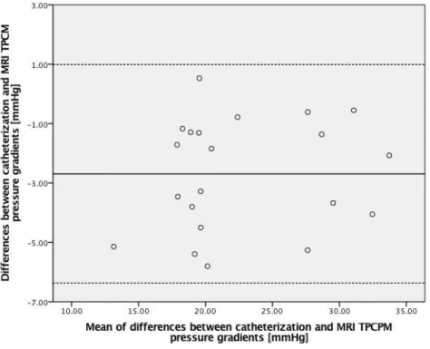
From the Bland-Altman approach is possible to verify the measurements from catheterization (22.86±6.64 mmHg) and MRI (25.47±6.68 mmHg), have a good agreement. The bias (mean of differences) is -2.59 mmHg and the limit of agreement (double of the standard deviation) is ±4.74 mmHg (Figure 15). This approach also shows that Doppler Echocardiography (27.15±11.43 mmHg) overestimates the catheterization measurements. The bias is -19.25 mmHg and the limit of agreement is ±30.16 mmHg. The linear correlation equation between catheterization and TCPM measurements is 𝑇𝐶𝑃𝑀 = 0.94 𝐶𝑎𝑡ℎ𝑒𝑡𝑒𝑟𝑖𝑧𝑎𝑡𝑖𝑜𝑛 + 3.93 and the linear equation between catheterization and Doppler echocardiography is 𝐷𝑜𝑝𝑝𝑙𝑒𝑟echocardiography = 0.66 𝐶𝑎𝑡ℎ𝑒𝑡𝑒𝑟𝑖𝑧𝑎𝑡𝑖𝑜𝑛 + 23.82_.

Figure 15-Bland Altman analysis to compare catheterization and MRI TCPM. The bias is -2.59 mmHg and the limitis ±4.74mmHg.

(39)

21

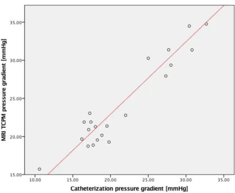
Figure 16-Scatterplot of the measurements from catheterization and MRIin mmHg. The red line is the trend line of the linear correlation between the two methods. The correlation coefficient between both absolute measures (catheter and MRI) is 0.88. The correlation equation is 𝑪𝑴𝑹=𝟎.𝟗𝟒𝑪𝒂𝒕𝒉𝒆𝒕𝒆𝒓𝒊𝒛𝒂𝒕𝒊𝒐𝒏+𝟑.𝟗𝟑

Figure 17 - Bland Altman analysis to compare catheterization and Doppler Echocardiographymeasurements. The bias is -19.25 mmHg and the limit is ±30.16 mmHg.