A Work Project, presented as part of the requirements for the Award of a Master Degree in Economics / Finance / Management from the NOVA – School of Business and Economics.
Does the European quantitative easing has an impact
on the targeted securities liquidity premium?
Simon Varsi 845
A Project carried out on the Master in Economics Program, under the supervision of: Professor André Silva
Abstract
We argue that large-scale asset purchases of the ECB lead to a decrease of the priced frictions in the targeted securities through a transmission channel. More precisely, we study the effect of the purchases of the inflation-linked central government bonds included in the European QE on the ILGB and inflation swap markets. Based on the liquidity transmission channel described by Christensen and Gillan (2016), we find that even if there is an evidence of this impact, it is not as huge as the one observed on the American market. We find that the difference in the liquidity premium varies from -0.024 to -1.152 basis points at five-year maturity, and from 0.166 to -1.182 basis points at ten-year maturity.
Keywords: European QE, Liquidity premium, Inflation-Linked Central Government Bond, Inflation swap, liquidity transmission channel
Table of contents
1. Introduction ... 4
American monetary policy ... 4
European response ... 4
How does European QE affect the liquidity premium in the targeted securities? ... 5
2. The particularities of the European QE and the liquidity channel ... 6
Liquidity transmission channels ... 6
Liquidity effects ... 7
Inflation-linked central government bond ... 8
European QE program ... 8
3. Methodology ... 10
Liquidity premium ... 10
Control variables ... 12
Standard Regression ... 13
Regression with a switch in conditional mean ... 15
4. Results ... 18
Empirical results ... 18
Comparison with the American’s QE2 ... 19
Discussion ... 19
5. Conclusion ... 21
1. Introduction
American monetary policy
The Great Recession induced by the global financial crisis of 2007-2009 led to an aggressive response from the Federal Reserve to stimulate the economy. The Federal Open Market Committee (FOMC) drove the target policy rate to its zero lower bound, and implemented a purchase of large-scale assets. According to the work of Gagnon, Raskin, Remache and Sack (2010), Christensen and Rudebusch (2012) and Krishnamurthy and Vissing-Jorgensen (2011) which analyzed the efficiency of these unusual monetary policies on the treasury yields and mortgage rates, the Federal Reserve’s large-scale asset purchases program was successful at stimulating the economic activity. Especially by reducing the term premium and improving market liquidity. Therefore, European Central Bank decided to implement the same kind of measures in order to revive its Economy.
European response
Indeed, the European Central Bank introduced the Public-Sector Purchase Programme (PSPP) on the 9th of March 2015. The objectives of this Quantitative Easing as set up in the ECB report by Mario Draghi (2015) are several. The main one remains the control of inflation at a rate lower but close to 2%. The second one is to low treasury yields to stimulate investment with a cheaper cost of borrowing. He also specified that he will continue to apply such a monetary policy until he reaches the objectives.
In this work, we explore the effect of this policy on the liquidity premiums of the inflation-linked central government bond and inflation swap markets. Several works find different outputs.
Korniyenko and Loukoianova (2015) analyzed the impact of the different QE in the USA, Europe, UK and Japan on the market liquidity, finding positive effect on global liquidity in USA and Europe while Arias and Wen (2014) argue that the large-scale asset purchases implemented by the FED created a liquidity trap: the excess of liquidity is hoard instead of spent which finally not increase liquidity and influence negatively the inflation.
How does European QE affect the liquidity premium in the targeted securities? This work is organized in the following way. The next section presents the particularities of the European QE and the liquidity transmission channels. Indeed, in this section, we explain the liquidity transmission channels through the ones the QE influence the long-term interest rates, and analyze the liquidity effects. Then we describe the inflation-linked central government bonds and their importance in the measure of the liquidity premiums. Finally, we see how the European QE meet the requirements needed to study its impact on the liquidity premiums.
In the section 3, we present our methodology. First, we describe and explain all the variables needed to run the regressions: the dependent variable which is the liquidity premium measure and the four control variables. We finally define the models use for the regressions (standard regression and regression with switch in the conditional mean), and the tables summarizing our findings.
The section 4 is composed of three subsections. They present the empirical results, whether there is an evidence of an impact of the QE on the liquidity premium measure. We compare these results with the ones found for the American QE2 and highlight the similarities and differences. Finally, we discuss about the possible causes leading to different findings.
The sections 5, 6, and 7 are respectively our conclusion, the references used for this work and the main appendices. The other appendices are displayed in another document.
2. The particularities of the European QE and the liquidity channel Liquidity transmission channels
The literature review gives us a theoretical overview of the liquidity channels used by the policy makers to influence both inflation and employment. Indeed, the purpose of implementing a QE is to affect interest rates through diverse transmission channels. It exists two main channels presented in the work of Hausken and Ncube (2013). First, the signaling channel corresponds to the information given by Central Bank and consists in providing information about the future purchases program. By announcing large-scale long-term asset purchases, the Central Bank keeps interest low in the future and prevent from losses. The impact on interest rates happens through the yield curve. Second, the portfolio rebalance channel happens when the Central Bank buys assets held by the private sector. Therefore, changing the relative supply of the assets being purchased, the sellers may attempt to rebalance their portfolios by buying substitutes: assets with similar characteristics as the ones sold. The effect is an increase of the prices of the assets purchased by the Central Bank and their substitutes, thus a decrease in associated term premiums and yields. However, Christensen and Gillan (2016) present a novel channel we use in this work to capture the effect of the QE on the market liquidity and therefore liquidity premiums which represents investors’ require compensation for assuming the risk of having to liquidate a long position in the security prematurely at a disadvantageous price.
Since Central Banks want the interest rates to go down, they do not care about the price raise implied by their unusual monetary policy (QE). Consequently, they eliminate the downside risk of the targeted securities and therefore, investors by submitting bids in the QE purchase auctions are less likely to face a disadvantageous price. Hence, market participants accept a lower liquidity premium. We notice that the main difference with the previous transmission channel
resides in the announcement effect which should not matter for this one. Indeed, the investors are only able to sell the targeted securities once the QE gets started. Hence, we expect a reduction of the liquidity premiums consequently to the beginning of the program.
Liquidity effects
In order to measure the liquidity effects, we need repeated purchases of securities less liquid than treasury securities over long period and a suitable measure of the priced frictions in the purchased security markets. The European QE meets these requirements since it started in March 2015 and is still in process (twenty months). It also includes repeated purchases of a significant amount of Inflation-linked Central Government Bonds (ILGB). Moreover, we calculate the priced frictions out of ILGB yields and inflation swap rates. We use it to find evidence of the liquidity channel, acknowledging that signaling channel and portfolio balance channel may affect it as well. Thanks to the rational, forward-looking behavior of investors, these two effects arise in principle following the announcement of the QE program and not when this one is implemented. Therefore, we verify for significant change in yields at the announcement date. We find out that there is not significant change in yields (Table 1) and consequently ruled out the signaling, and portfolio balance effects as drivers of the variation in the measure of liquidity premiums in ILGB yields and inflation swap rates during the QE.
Response to QE announcement Maturity 5 Years 10 Years INGB BEI rates
Jan. 22, 2015 0.834 0.95
Jan. 23, 2015 0.834 0.91
Change 0 -0.04
Inflation swap rates
Jan. 22, 2015 0.301 0.706
Jan. 23, 2015 0.297 0.699
Change -0.004 -0.007
LP measure Jan. 22, 2015 Jan. 23, 2015 -0.533 -0.536 -0.244 -0.211
Change -0.003 +0.033
Nominal yields
Jan. 22, 2015 -0.021 0.366
Jan. 23, 2015 -0.022 0.454
Change -0.001 +0.088
Table 1 : Response to QE announcement. This table describes the change in our data due to the
announcement of the QE on the 22nd of January, 2015. All these data are rates so in percentage. The changes are never above 0.1%, we conclude that there is no significant change in our
dataset.
Inflation-linked central government bond
The European QE provides a good experiment for studying liquidity effects on the market of inflation-linked central government bond and the linked market of inflation swap. Indeed, the characteristics meet the requirements as seen in the previous section. Furthermore, Fleming and Krishnan (2012) argue in their work, that the characteristics in the ILGB market: smaller trading volume, wider bid-ask spreads and longer turnaround time than observed in the nominal bond market, are in favor of the existence of a liquidity premium.
European QE program
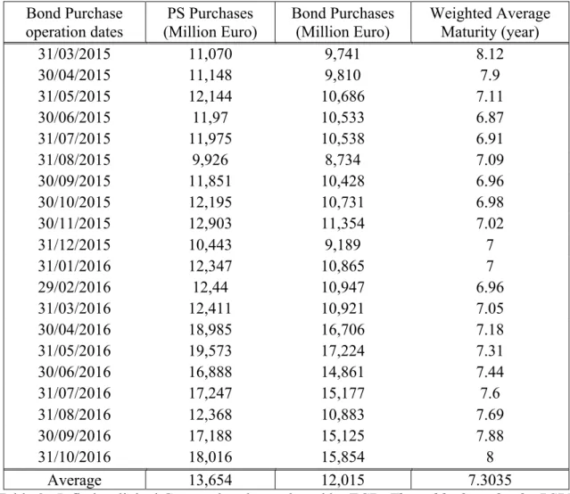
The expanded asset purchase program which was announced in January 2015, started from March 2015 and is supposed to end in March 2017. The ECB stated that it consists in average purchases in public and private sector securities of 80 billion euros per month. It includes the purchases of covered bond, asset-backed securities, corporate sector securities and public sector
securities. Inflation-linked central government bond belongs to the latest category mentioned. The purchase of bonds represents 72,974 million euros per month, so by far the most important asset category purchased by the ECB.
Bond Purchase operation dates PS Purchases (Million Euro) Bond Purchases (Million Euro) Weighted Average Maturity (year) 31/03/2015 11,070 9,741 8.12 30/04/2015 11,148 9,810 7.9 31/05/2015 12,144 10,686 7.11 30/06/2015 11,97 10,533 6.87 31/07/2015 11,975 10,538 6.91 31/08/2015 9,926 8,734 7.09 30/09/2015 11,851 10,428 6.96 30/10/2015 12,195 10,731 6.98 30/11/2015 12,903 11,354 7.02 31/12/2015 10,443 9,189 7 31/01/2016 12,347 10,865 7 29/02/2016 12,44 10,947 6.96 31/03/2016 12,411 10,921 7.05 30/04/2016 18,985 16,706 7.18 31/05/2016 19,573 17,224 7.31 30/06/2016 16,888 14,861 7.44 31/07/2016 17,247 15,177 7.6 31/08/2016 12,368 10,883 7.69 30/09/2016 17,188 15,125 7.88 31/10/2016 18,016 15,854 8 Average 13,654 12,015 7.3035
Table 2 : Inflation-linked German bonds purchased by ECB. This table describe the PSPP
implemented by the ECB in Germany. We notice the purchases arise in a regular basis (every month) and with large amounts. Indeed, the bond purchases which represent 88% of the total
amount of this program present an average of 12 Billion euros per months in Germany.
This program includes two types of securities: the bonds issued by recognized agencies, regional and local governments, international organizations and multilateral development banks located in the euro area (12%) and the ones which are interesting for this work: the nominal and
ILGB (88%). As a representation of Europe, we choose to study the purchases made in Germany (Table 2). Indeed, Germany benefits of the biggest amount of purchase and consequently gives us the best data to evaluate the Eurozone QE. Until now, 16 purchases were done on last day of every month.
3. Methodology
Liquidity premium
In this work, we use the liquidity premium measure created by Christensen and Gallan (2016). This measure is calculated out of two variables: it is the difference between the inflation swap rate and breakeven inflation rate. This measure captures the priced frictions in the inflation-linked German bond and inflation swap markets. Indeed, an inflation swap contract implied a fixed payment in exchange for a floating payment equal to the change in the CPI used in the inflation indexation of ILGB while the breakeven-inflation is the difference yield between regular nominal treasury bonds and ILGB of the same maturity. In a frictionless world, inflation swap rate is equal to the BEI rate because without arbitrage opportunity, buying one nominal discount bond today gives the same cash flow as buying one real discount bond and selling an inflation swap contract, all of them with the same maturity. But in the real economy, some frictions occur in the market. The difference between the frictionless world and the reality is therefore defined as the liquidity premium measure.
𝐿𝑃# 𝜏 = 𝐼𝑆# 𝜏 − 𝐵𝐸𝐼 𝜏 (1)
Where 𝐿𝑃# 𝜏 is the liquidity premium measure, 𝐼𝑆# 𝜏 is the inflation swap and 𝐵𝐸𝐼 𝜏 is the breakeven inflation. We take the inflation swap from the Bundesbank and the breakeven
inflation from Bloomberg. According to Pelata and Dent (2013), although they vary technically, these instruments both predict inflation since they reflect the inflation expectations.
Graphic 1 : Measure of liquidity premium from November 2009 to November 2016. The measure
of the liquidity premium, which is the difference between the inflation swap rate and the breakeven inflation rate describes the frictions in the inflation-linked German bonds and German
inflation swap markets. We can see that after the crisis these frictions were huge but slowly decreased since 2009. The difference is expressed in percentage.
This measure of liquidity premium combine the information in treasury yields, ILGB yields and inflation swap to isolate the liquidity premium from the inflation and monetary policy expectations. Indeed, since the cash flows of ILGB and inflation swaps are adjusted with the same German CPI, the connection between their pricing allow to reduce the part involved by the inflation and monetary policy.
In their work, Christensen and Gillan (2016) impose several conditions would lead to the restriction: the liquidity premium cannot be negative (Appendix). However, we can observe that is
2012 until now. We link this difference to the fact that Europe and Germany faced deflation expectations. The inflation swap rates enforce this hypothesis since it also becomes negative.
Other model-free measures of priced frictions exist. The most common alternative is the asset swap spreads used by Pflueger and Viceira (2013), but Christensen and Gillan (2016) demonstrates that this measure capture the same effect as the one use in this work, they are therefore highly correlated.
Control variables
The four variables which aim to control the liquidity premium in the ILGB and inflation swap markets and therefore the bond market liquidity are described below.
The first is the New-DAX Volatility Index, it is the implied volatility of the DAX anticipated on the derivatives market. It represents uncertainty and risk-aversion about the near future of the general stock market as reflected in options in the DAX price index. We include this variable since an increased uncertainty about the future prices could drive the liquidity premium up. Hence, a positive change in the VDAX is expected to lead to an increase in the liquidity premium
The second is the Illiquidity premium. As describe in the work of Amihud (2002), the stock excess return (risk premium) is in part a premium for illiquidity, thus we decide to use the excess stock return of the DAX Index as a control variable. A positive change in the excess stock return should imply a decrease in the liquidity premium.
The third is the yield difference between seasoned (off-the-run) Treasury securities and the most recently issued (on-the-run) Treasury security of the same maturity. This spread capture the
liquidity premium in the treasury bond market, thus we expect to see a comparable movement in the liquidity premium in ILGB yield and inflation swap rates.
The last one is the bid-ask spreads Euro swap. The frictions represented in this spread can capture a part of variation in our liquidity premium measure. Indeed, it represents the uncertainty about the future inflation.
For the two last control variables, we use the 5-Years and 10-Years maturities we will separately use for the liquidity premium 5-Years and 10-Years maturities regressions. All the data used for the regression goes from the 10th of June, 2009 to the 11th of November 2016. The values in parentheses represent the T-statistic values while ** means the coefficient is statistically significant at a 99% level of confidence, * at a 95% level of confidence and without any star means that the coefficient is not significant.
Standard Regression
To test the impact of our explanatory variables on the dependent variable, we use standard regressions at both five-year and ten-year maturities (Table 3 and 4) with, as a dependent variable,
our measure of liquidity premium 𝐿𝑃# 𝜏 on the four control variables describe above: The
New-DAX volatility 𝑉𝐷𝐴𝑋#, the 30-days moving average of the DAX excess returns
𝑀𝐴𝐸𝑥𝑐𝑒𝑠𝑠𝑅𝑒𝑡𝑢𝑟𝑛#, the off-the-run spread 𝑂𝑓𝑓𝑡ℎ𝑒𝑅𝑢𝑛𝑆𝑝𝑟𝑒𝑎𝑑# 𝜏 , and finally the bid-ask spread
on the currency swap 𝐵𝑖𝑑𝑎𝑠𝑘𝑆𝑝𝑟𝑒𝑎𝑑# 𝜏 . The 𝜏 represents the maturity.
𝐿𝑃# 𝜏 = 𝛽C+ 𝛽E𝑉𝐷𝐴𝑋# (2)
𝐿𝑃# 𝜏 = 𝛽C+ 𝛽F𝑀𝐴𝐸𝑥𝑐𝑒𝑠𝑠𝑅𝑒𝑡𝑢𝑟𝑛# (3)
𝐿𝑃# 𝜏 = 𝛽C+ 𝛽H𝐵𝑖𝑑𝑎𝑠𝑘𝑆𝑝𝑟𝑒𝑎𝑑# 𝜏 (5)
𝐿𝑃# 𝜏 = 𝛽C+ 𝛽F𝑀𝐴𝐸𝑥𝑠𝑠𝑅𝑒𝑡𝑢𝑟𝑛#+ 𝛽G𝑂𝑓𝑓𝑅𝑢𝑛𝑆𝑝𝑟𝑒𝑎𝑑# 𝜏 (6)
𝐿𝑃# 𝜏 = 𝛽C+ 𝛽E𝑉𝐷𝐴𝑋#+ 𝛽F𝑀𝐴𝐸𝑥𝑠𝑠𝑅𝑒𝑡𝑢𝑟𝑛#
+𝛽G𝑂𝑓𝑓𝑅𝑢𝑛𝑆𝑝𝑟𝑒𝑎𝑑# 𝜏 + 𝛽H𝐵𝑖𝑑𝑎𝑠𝑘𝑆𝑝𝑟𝑒𝑎𝑑# 𝜏 (7)
Following the individual regressions (1) to (4) the explanatory variables gave us the expected signs beside the bid-ask Spread on the Euro swap which is not significant at five-year
maturity and negative at ten-year maturity. Moreover, it has no explanatory power (R2=-0.0005
and 0.0059). As predicted, a positive change in the 30-day moving average of the DAX excess return makes the liquidity premium decreases and a positive change in the off-the-run spread makes the liquidity premium increases. These two variables have the strongest effect on the dependent variable (respectively -1.048 and -1.012 for the first one and 0.797 and 0.694 for the second one) and remain highly significant with the greatest explanatory power. The other variables are marginal factors in explaining the variation of the dependent variable. Indeed, in addition of a poor explanatory power, the VDAX and the Bid-Ask Spread on the Euro swap even change their sign from the individual regressions (1) and (4) to the baseline one (6). We verify this hypothesis with the regression (5) which almost has the same explanatory power than the baseline one for both five-year and ten-year maturities.
Tables 3 and 3: These tables describe all the standard regressions done at five-year and ten-year
maturities. For a positive change of one basis point of percentage in the explanatory variable, the liquidity premium will change in average by the concerned value in the table (percentage). The R2 define the explanatory power of the regression. This model describes the control of the explanatory variables on the liquidity premium measure. **: p<0.01, *: p<0.05. The values in
parentheses is the t-statistic.
Explanatory variables Dependent variable: Liquidity Premium measure 5-Year maturity
(2) (3) (4) (5) (6) (7)
Constant 0.394** 0.107** -0.300** 0.369** -0.270** -0.652**
(-6.45) (12.04) (-45.87) (9.15) (-33.78) (-32.08)
VDAX 0.033** 0.015**
(12.89) (21.86)
30-day MA Stock excess return -1.048** -0.11** -0.041**
(-81.20) (-6.54) (-2.66)
Off-the-run spread 0.797** 0.727** 0.754**
(151.06) (61.61) (70.88)
Currency SWAP bid-ask spread -0.247 1.35**
(-0.16) (3.63)
Adjusted R2 0.0787 0.7734 0.9220 -0.0005 0.9384 0.9388
Explanatory variables Dependent variable: Liquidity Premium measure 10-Year maturity
(2) (3) (4) (5) (6) (7)
Constant -0.223** 0.262** -0.640** 0.613** -0.541** -0.849**
(-3.70) (28.09) (-65.66) (18.12) (-38.49) (-35.57)
VDAX 0.032** 0.015**
(12.63) (21.32)
30-day MA Stock excess return -1.012** -0.152** -0.041**
(-74.40) (-9.53) (-6.23)
Off-the-run spread 0.694** 0.612** 0.630**
(139.13) (61.89) (71.19)
Currency SWAP bid-ask spread -5.320** -2.948**
(-3.54) (-7.45)
Regression with a switch in conditional mean
In order to see if the QE had an impact on liquidity premium of the targeted securities, we run a regression imposing a change in conditional mean following the European QE announcement (Table 5 and 6). To do so, we include two dummy variables 𝛿𝑝𝑟𝑒𝑄𝐸 which takes the value 1 until the 26th of January, 2015 or 0 otherwise and 𝛿𝑝𝑜𝑠𝑡𝑄𝐸 which takes the value 1 from the 26th of January 2015 or 0 otherwise. The result is the creation of two constants, one before the announcement 𝛿𝑝𝑟𝑒𝑄𝐸 and the other one afterwards 𝛿𝑝𝑜𝑠𝑡𝑄𝐸. A switch of sign in the constants would mean that the QE had an impact on the market liquidity. Therefore, we expect the constant to switch from positive before the announce to negative afterwards.
𝐿𝑃# 𝜏 = 𝛽C𝛿𝑝𝑟𝑒𝑄𝐸 + 𝛽E𝛿𝑝𝑜𝑠𝑡𝑄𝐸 + 𝛽F𝑉𝐷𝐴𝑋# (8) 𝐿𝑃# 𝜏 = 𝛽C𝛿𝑝𝑟𝑒𝑄𝐸 + 𝛽E𝛿𝑝𝑜𝑠𝑡𝑄𝐸 + 𝛽G𝑀𝐴𝐸𝑥𝑐𝑒𝑠𝑠𝑅𝑒𝑡𝑢𝑟𝑛# (9) 𝐿𝑃# 𝜏 = 𝛽C𝛿𝑝𝑟𝑒𝑄𝐸 + 𝛽E𝛿𝑝𝑜𝑠𝑡𝑄𝐸 + 𝛽H𝑂𝑓𝑓𝑡ℎ𝑒𝑅𝑢𝑛𝑆𝑝𝑟𝑒𝑎𝑑# 𝜏 (10) 𝐿𝑃# 𝜏 = 𝛽C𝛿𝑝𝑟𝑒𝑄𝐸 + 𝛽E𝛿𝑝𝑜𝑠𝑡𝑄𝐸 + 𝛽L𝐵𝑖𝑑𝑎𝑠𝑘𝑆𝑝𝑟𝑒𝑎𝑑# 𝜏 (11) 𝐿𝑃# 𝜏 = 𝛽C𝛿𝑝𝑟𝑒𝑄𝐸 + 𝛽E𝛿𝑝𝑜𝑠𝑡𝑄𝐸 + 𝛽G𝑀𝐴𝐸𝑥𝑠𝑠𝑅𝑒𝑡𝑢𝑟𝑛#+ 𝛽H𝑂𝑓𝑓𝑅𝑢𝑛𝑆𝑝𝑟𝑒𝑎𝑑# 𝜏 (12) 𝐿𝑃# 𝜏 = 𝛽C𝛿𝑝𝑟𝑒𝑄𝐸 + 𝛽E𝛿𝑝𝑜𝑠𝑡𝑄𝐸 + 𝛽F𝑉𝐷𝐴𝑋# +𝛽G𝑀𝐴𝐸𝑥𝑠𝑠𝑅𝑒𝑡𝑢𝑟𝑛#+ 𝛽H𝑂𝑓𝑓𝑅𝑢𝑛𝑆𝑝𝑟𝑒𝑎𝑑# 𝜏 + 𝛽L𝐵𝑖𝑑𝑎𝑠𝑘𝑆𝑝𝑟𝑒𝑎𝑑# 𝜏 (13)
Explanatory variables Dependent variable: Liquidity Premium measure 5-Year maturity
(8) (9) (10) (11) (12) (13)
Constant pre-QE announcement -0.255** 0.203** -0.288** 0.813** -0.259** -0.611**
(-5.63) (17.64) (-29.65) (24.05) (-24.52) (-29.74)
Constant post-QE announcement -1.407** -0.081** -0.312** -0.318** -0.280** -0.706**
(-27.04) (-4.68) (-31.39) (-8.62) (-25.40) (-31.90)
VDAX 0.040** 0.016**
(20.58) (22.69)
30-day MA Stock excess return -0.938** -0.110** -0.034*
(-61.37) (-6.53) (-2.20)
Off-the-run spread 0.789** 0.721** 0.729**
(115.57) (57.97) (65.82)
Currency SWAP bid-ask spread -7.217** 0.68
(-6.09) (1.81)
Adjusted R2 0.5855 0.8288 0.9362 -0.5040 0.9375 0.9507
Explanatory variables Dependent variable: Liquidity Premium measure 5-Year maturity
(8) (9) (10) (11) (12) (13)
Constant pre-QE announcement -0.083 0.39** -0.763** 0.94** -0.661** -0.872**
(-1.92) (33.04) (-48.30) (34.94) (-33.76) (-33.99)
Constant post-QE announcement -1.265** 0.011 -0.597** -0.199** -0.515** -0.819**
(-25.48) (0.63) (-56.70) (-5.97) (-36.39) (-33.39)
VDAX 0.038** 0.015**
(21.13) (19.59)
30-day MA Stock excess return -0.864** -0.134** -0.089*
(-55.04) (-8.49) (-6.11)
Off-the-run spread 0.744** 0.666** 0.648**
(105.37) (57.69) (61.68)
Currency SWAP bid-ask spread -8.125** -2.903
(-7.13) (-7.29)
Adjusted R2 0.6735 0.8436 0.9405 0.6083 0.9426 0.9536
Tables 5 and 4: These table describe all the regressions with a change in the conditional mean
done at five-year and ten-year maturities. For a positive change of one basis point of percentage in the explanatory variable, the liquidity premium will change in average by the concerned value
in the table (percentage). The R2 define the explanatory power of the regression. This model describes the impact of the announce on the liquidity premium measure. **: p<0.01, *: p<0.05.
4. Results
Empirical results
First, we see a little increase in the adjusted R2 values from the regressions without switch in conditional mean to the last ones with the switch. Second, the changes in the explanatory variables are tiny following the addition of the switch in the conditional mean, this encourages the choice not to allow for any switch in their effects on the liquidity premium measure. Third, a measure of the persistent negative effect of the Inflation-linked German bonds purchase on the liquidity premium measure is the difference in the estimated constant terms. Still from table 5 and 6, we observe that the differences at five-year maturity go from -0.024 to -1.152 basis points while at ten-year maturity, they go from 0.166 to -1.182 basis points. Finally, we test the hypothesis that there is no change in the constant term after the announcement of the QE program. This is done with F-test which says that this hypothesis is rejected at a 99.99% of confidence level at both maturities.
From an empirical point of view, the results are not clear, indeed even though there is evidence of a change in the conditional mean, this one is not big. While looking at graphic 1, we can see that the main change in the conditional mean happened in three parts from 2009 to 2015. We also observe that when the European QE is announced, the liquidity premium is already near to zero. Then the implementation of the large-scale purchases by the ECB pushes the liquidity premium under zero. We are now going to compare these results with the one found in the work of Christensen and Gillan (2016), concerning the American QE2.
Comparison with the American’s QE2
Right after the financial crisis of 2008, the Federal Reserve implemented its QE, however it started to purchase Inflation-linked central government bonds during its second QE. The analyze of the impact of these purchase on the liquidity premium in these securities market revels that the announce of the QE2 had a big impact, steeply pushing down the constant of the liquidity premium. These results are confirmed by a counterfactual analysis added at their work. They found out that the QE2 persistently reduces the liquidity premium measure by an average of 10 to 13 basis points but the most interesting is the disappearance of this effect towards the end of the program. Indeed, that suggests the effect of the purchases is present only when these one are ongoing or expected to remain ongoing. We unfortunately cannot perceive this phenomenon in our model since the program is still in progress and might be extended even though Mario Draghi did not give any information about it, per the Wall street journal (2016). The decision should be given in December. In the next section, we discuss of the possible reason explaining why it exists such differences between the impacts of the QE.
Discussion
The timing of the QE matters, indeed, in the USA we observe that the first QE was implemented right after the financial crisis while the ECB waited until 2015 to start its own. It has a huge impact on the findings because the first QE of the FED limited the impact of the crisis on the American economy and as described in the work of Kurov (2009), the decisions made by the Central Bank has positive effect on investor sentiment. Therefore, when they implemented the QE2, there were not unusual movement on the treasury inflation-protected securities market. Contrariwise, in Europe, the inaction of the ECB did not limit the impact of the crisis. Moreover,
the Eurozone face a sovereign debt crisis since many years (Greek crisis for instance). This climate of fear makes investors go to the safest assets like ILGB. This pushes the liquidity premiums down by the same transmission channel used in our model. This effect is even greater in our model since we take Germany which is the safest country of the zone as a representative for Europe. We observe this effect on the graphic 1, with the downward slope of the liquidity premium measure from 2009. The effect of the European QE could have been reduced by the announcement of this one. Indeed, the ECB displayed confidence in the future and as seen before gave a positive sentiment to investors who then came back on the stock market. This phenomenon might increase the liquidity premium in the ILGB market since investors left this market. The stock market reaction after the announcement of the European QE: increase of the DAX30 index, enforces this hypothesis (Graphic 2).
Graphic 2: DAX 30. This graphic describes the movement of the DAX30 (German stock
exchange) from June 2014 to June 2016. The aim is to capture the change in the stock exchange due to the announcement of the QE. The value of the DAX30 is points.
In his work, Elliot argues that the factor which could reduce liquidity in the market are the Basel III capital accord which regulate more the markets and make the business more expensive for banks and major securities dealers, the single counterparty credit limits which tighten the credit exposure of the banks and the Volcker rule, which prohibits the banks from engaging in proprietary trading.
5. Conclusion
In this work, we argue that the large-scale asset purchases of the ECB lead to a decrease of the priced frictions in the targeted securities through a transmission channel. More precisely, we study the effect of the purchases of the inflation-linked central government bonds included in the European QE which got started in March 2015 on the liquidity premiums in the ILGB and inflation swap markets.
To highlight this relationship, we first describe the liquidity transmission channels. The two main channels are the signaling and portfolio rebalance channels. We put in evidence that the effects of these channels which should appear after the announcement have no influence on the liquidity premium measure. Therefore, we analyze the impact of the QE through the transmission channel described by Christensen and Gillan (2016). We verify that the European QE satisfy all the requirements: purchases of inflation-linked central government bonds must be large enough and make on a regular basis.
To empirically demonstrate this relationship, we use a measure of the liquidity premium created by Christensen and Gillan (2016) as a dependent variable. We then use four explanatory variables: The New-DAX Volatility Index, a measure of illiquidity (30-day moving average of the excess return of DAX Index), the off-the-run spread which is the yield difference between seasoned treasury securities and the most recently issued and finally the bid-ask spread of the Euro swap.
The regression with a switch in conditional mean which was the one capturing the desired effect suggests that the purchases of inflation-linked German bonds reduce a little bit the priced frictions in the ILGB and inflation swap markets. Indeed, compared to the reductions observed after the American QE, the evidence of benefits from the QE on the financial market in Europe is small. The fact that the QE is not over yet does not allow us to witness the behavior of the liquidity premium after the end of the program.
We discussed then of the possible reasons inducing these low results. The ones which came in our minds are the timing of the QE implementation and the effect of its announcement. Indeed, The European QE came late after the American one which created an atmosphere of fear. This pushed the investors on the safest markets and ILGB is part of them. Therefore, it drove the liquidity premium down before the announcement of the QE, making our result less relevant. Furthermore, as presented in Kurov’s work (2009), the announcement created a positive sentiment in the market. Hence, the investors got back on the stock market instead of the bond market. This effect could have lead the liquidity premium up, cancelling the effect of the purchases in our regression.
However, there is no evidence of these effects in this work. There are only hypothesis and need to be tested in further researches.
6. References
Amihud, Yakov. 2002. « Illiquidity and stock returns: cross-section and time-series effects ». Journal of financial markets, 5: 31-56
Arias, Maria A. and Yi Wen. 2014. « The liquidity trap: An alternative explanation for today’s low inflation ». The regional economist, April 2014: 10-11
Christensen, Jens H.E. and Glenn D. Rudebusch. 2012. « The Response of Interest Rates to U.S. and U.K. Quantitative Easing ». Federal Reserve Bank of San Francisco Working Paper Series, 2012-06
Christensen, Jens H.E. and James Gillan. 2016. « Does Quantitative Easing Affect Market Liquidity? ». Federal Reserve Bank of San Francisco Working Paper, 2013-26
Claeys, Grégory and Álvaro Leandro. 2016. « The European Central Bank’s quantitative easing programme: Limits and risks ». Bruegel Policy Contribution, 2016-04
Draghi, Mario. 2015. « Introductory statement to the press conference (with Q&A) ». Available at: http://www.ecb.europa.eu/press/pressconf/2015/html/is150122.en.html
Elliott, Douglas J. 2015. « Market liquidity: A primer ». Economics Studies at Brookings, June 2015
European Central Bank. 2015. « Asset purchase programme ». Available at: http://www.ecb.europa.eu/mopo/implement/omt/html/index.en.html
Fleming, Michael J. and Neel Krishnan. 2012. « The microstructure of the TIPS market ». Federal Reserve Bank of New York Economic Policy Review, Vol 18(1): 27-45
Financial Times. 2015. « German bonds measure success of Eurozone QE ». Available at:
https://www.ft.com/content/f297129a-ee7b-11e4-88e3-00144feab7de
Gagnon, Joseph, Matthew Raskin, Julie Remache, and Brian Sack. 2010. « Large-Scale Asset Purchases by the Federal Reserve: Did They Work? ». Federal Reserve Bank of New York Economic Policy Review, 17(1): 41-59
Garcia, Juan Angel and Adrian Van Rixtel. 2007. « Inflation-linked bonds from a central bank perspective ». European Central Bank Occasional Paper series, 2007-62
Garcia, Juan Angel and Thomas Werner. 2010. « Inflation risks and inflation premia ». European Central Bank Working Paper series, 2010-1162
Hausken, K. and M. Ncube. 2013. « Transmission Channels for QE and Effects on Interest Rates » in Quantitative Easing and its Impact in the US, Japan, the UK and Europe ed. Springerbriefs in Economics, 5-6. New York: Springer-Verlag
Korniyenko, Yevgeniya and Elena Loukoianova. 2015. « The Impact of Unconventional Monetary Policy Measures by the Systemic Four on Global Liquidity and Monetary Conditions ». IMF Working Paper, WP/15/287
Krishnamurthy, Arvind and Annette Vissing-Jorgensen. 2011. « The effects of quantitative easing on interest rates ». Brookings Papers on Economics Activity, Fall 2011: 215-265
Kurov, Alexander. 2009. « Investor sentiment and the stock market’s reaction to monetary policy ». Journal of banking and finance, Vol 34(1): 139-149
Pelata, Marion and Adam Dent. 2013. « Mastering inflation linkers and derivatives: overview of European and UK inflation markets ». Credit Suisse securities research and analytics, September2013
Pflueger, Carolin E. and Luis Viceira. 2013. « Return predictability in the treasury market: real rates, Inflation and liquidity». Manuscript, Harvard Business School
The Wall Street Journal. 2016. « ECB’s Mario Draghi Hints at Extension of Bond Purchases ». Available at:
7. Appendix 𝐿𝑃# 𝜏 = 𝐼𝑆# 𝜏 − 𝐵𝐸𝐼 𝜏 𝐿𝑃# 𝜏 = 𝐼𝑆# 𝜏 − [𝑦#O 𝜏 − 𝑦 #P 𝜏 ] 𝐿𝑃# 𝜏 = 𝐼𝑆# 𝜏 + 𝛿#RS 𝜏 − [𝑦 #O 𝜏 − (𝑦#P 𝜏 + 𝛿#P 𝜏 )] 𝐿𝑃# 𝜏 = 𝛿#RS 𝜏 + 𝛿 #P 𝜏 ≥ 0
Where 𝐿𝑃# 𝜏 is the liquidity premium, 𝐼𝑆# 𝜏 is the inflation swap and 𝛿#RS 𝜏 its
time-varying liquidity premium, 𝐵𝐸𝐼 𝜏 is the breakeven inflation, 𝑦#O 𝜏 and 𝑦
#P 𝜏 are respectively
the nominal and the real treasury zero-coupon bond yields, and 𝛿#P 𝜏 is the time-varying liquidity