Dosimetric Effects of Clinical Setup Mismatch in Volumetric Modulated Arc Therapy as Assessed by Monte Carlo Methods

(1)

Dosimetric Effects of

Clinical Setup

Mismatch in

Volumetric

Modulated Arc

Therapy as Assessed

by Monte Carlo

Methods

Ricardo José Pires Magalhães

Dissertação de Mestrado apresentada à

Faculdade de Ciências da Universidade do Porto em

Física Médica

2018

Dosimetric Effects of Clinical Setup Mismatch in

Volumetric Modulated Arc Therapy as Assessed by

Monte Carlo Methods

Ricardo José Pires Magalhães

FCUP 2018

2.º CICLO

(2)

Dosimetric Effects of

Clinical Setup

Mismatch in

Volumetric

Modulated Arc

Therapy as Assessed

by Monte Carlo

Methods

Ricardo José Pires Magalhães

Mestrado em Física Médica

Departamento de Física e Astronomia 2018

Orientador

Carla Carmelo Rosa, Professora Auxiliar, Faculdade de Ciências da Universidade do Porto

Coorientador

Joana Lencart, Especialista em Física Médica, Instituto Português de Oncologia do Porto de Francisco Gentil

(3)

O Presidente do Júri,

(4)

i

Acknowledgements

This work was only possible due to the collaboration and support of several people and institutions. Therefore I would like to thank all those who contributed to its realization:

To the University of Porto in the name of the Magnificent Rector António de

Sousa Pereira.

To the Faculty of Sciences of the University of Porto in the name of the

Director, Professor Doutor António Fernando Silva.

To the Instituto Português de Oncologia do Porto de Francisco Gentil, to the Instituto Português de Oncologia do Porto de Francisco Gentil Research

Center, and to the Department of Physics and Astronomy for the availability of the

facilities, materials, and equipment needed to carry out this work.

To Professora Doutora Carla Carmelo Rosa my thesis supervisor, and to

Doutora Joana Lencart my thesis co-supervisor, who for their help, attention,

dedication, guidance, and availability have allowed me to improve my knowledge. To Professor Doutor Joaquim Agostinho Gomes Moreira for the guidance in the improvement of my academic training in physics and mathematics.

To the PhD Students Jorge Oliveira and Firass Ghareeb for all the help, suggestions, and clarification of doubts whenever they came to me.

To my family for the unconditional support over the years and without which any of this work would be possible.

Finally, to my friends who provided me a great support for the conclusion of this stage.

(5)

ii

Resumo

Atualmente a radioterapia é uma das principais modalidades usadas no tratamento do cancro, sendo que diversas técnicas têm vindo a ser desenvolvidas nesta área de forma de aumentar a precisão no fornecimento de dose e, simultaneamente, minorar a probabilidade de efeitos secundários para o paciente. A radioterapia de intensidade modulada (IMRT) e a terapia em arco volumétrico (VMAT) aparecem com particular relevância neste contexto, visto permitirem reduzir o tempo de tratamento assim como melhorar a conformação da distribuição de dose ao volume alvo.

Um dos aspectos mais críticos no processo de radioterapia é o posicionamento do paciente na mesa de tratamento, pois um desvio na sua localização poderá levar a uma redução da dose fornecida ao volume alvo e a um incremento da dose recebida pelos tecidos saudáveis, aumentando a probabilidade de complicações para o indivíduo. Assim existe o interesse em avaliar os efeitos dosimétricos no paciente resultantes de desvios do seu posicionamento.

O cálculo da distribuição de dose no interior do corpo humano é um processo complexo, sendo que actualmente o método de Monte Carlo é considerado a abordagem mais apropriada a este problema. Neste contexto, o PRIMO surge como um programa para aplicação dessa metodologia ao cálculo da dose fornecida a um volume, também incluindo uma interface gráfica que facilita o seu uso na prática clínica. Assim sendo, o trabalho desenvolvido teve como principal objectivo avaliar os efeitos dosimétricos decorrentes de desvios no posicionamento na técnica de VMAT, através da utilização do método de Monte Carlo.

Com este propósito foram realizadas várias tarefas, nomeadamente a validação de um espaço de fase para o acelerador linear TrueBeamTM instalado no IPOPFG relativo à energia de fotões de 6MV com filtro aplanador, a validação do modelo do MLC fornecido pelo PRIMO, o estudo dos mecanismos de simulação aplicados no PRIMO para a simulação de planos de IMRT e VMAT e a análise dos efeitos dosimétricos, em VMAT, resultantes de vários desvios no posicionamento de modo a estabelecer as condições críticas para a localização do paciente na mesa do TrueBeamTM em operação no IPOPFG.

Por fim, foi desenvolvido um protocolo de adaptação do plano de tratamento a eventuais desvios no posicionamento, tendo por base a informação recolhida durante o trabalho realizado.

(6)

iii

Abstract

Currently radiotherapy is one of the main modalities used in the treatment of cancer. Several techniques have been developed in this area as a way to increase the precision in the dose delivery and, simultaneously, to diminish the probability of side effects for the patient. Intensity modulated radiotherapy (IMRT) and volumetric arc therapy (VMAT) appear with particular relevance in this context, because they can reduce the treatment time as well as improve the conformation of the dose distribution to the target volume.

One of the most critical aspects associated to the radiotherapy process is the patient positioning on the treatment couch, since a deviation in their location may lead to a reduction of the dose delivered to the target volume and to an increase of the dose received by the healthy tissues, augmenting the probability of complications for the individual. Consequently, the interest on evaluating the dosimetric effects in the patient resulting from deviations of their positioning surges.

The calculation of the dose distribution inside the human body is a complex process, being the Monte Carlo method currently considered the most appropriate approach to such problem. In this context, PRIMO appears as a program for the application of that methodology to the calculation of the dose delivered to a volume, also including a graphical interface that facilitates its use in the clinical practice. As a result, the main objective of the work done was to evaluate the dosimetric effects resulting from positioning deviations in the VMAT technique through the application of the Monte Carlo method.

With this purpose several tasks were performed, namely the validation of a phase space for the TrueBeamTM linear accelerator installed in IPOPFG relative to 6MV photon energy with a flattening filter, the validation of the MLC model provided by PRIMO, the study of the simulation mechanisms applied in PRIMO for the simulation of IMRT and VMAT plans, and the analysis of the dosimetric effects, in VMAT, resulting from various positioning shifts with the view to establish the critical conditions of the patient location on the treatment couch of the TrueBeamTM operating at IPOPFG.

Finally, a protocol to adapt the treatment plan to eventual positioning mismatches was developed, based on the information collected during the work performed.

(7)

iv

Keywords

External Beam Radiotherapy; External Radiotherapy; Radiotherapy; Adaptive Radiotherapy; Varian; TrueBeam; VMAT; IMRT; Setup; Positioning; Dosimetry; Monte Carlo; Simulation; PRIMO; PENELOPE

(8)

v

Index

1.) Introduction ... 1

1.1.) Motivation ... 1

1.2.) Thesis Outline ... 2

2.) Theoretical and Experimental Background ... 3

2.1.) Radiobiological Background ... 3

2.2.) Radiation Physics ... 4

2.2.1.) Interaction of Electrons with Matter ... 4

2.2.2.) Interaction of Photons with Matter ... 6

2.2.2.1.) Photon Attenuation Coefficients ... 11

2.2.3.) Basic Quantities and Units in Radiation Dosimetry ... 12

2.2.3.1.) Particle Number and Radiant Energy ... 12

2.2.3.2.) Flux and Energy Flux ... 12

2.2.3.3.) Fluence and Energy Fluence ... 13

2.2.3.4.) Fluence Rate and Energy-Fluence Rate ... 13

2.2.3.5.) KERMA ... 13

2.2.3.6.) Absorbed Dose ... 14

2.2.3.6.1.) Charged Particle Equilibrium (CPE) ... 15

2.2.3.7.) Exposure (X) ... 16

2.3.) The Linear Accelerator ... 17

2.4.) The Flattening Filter Free Mode ... 20

2.5.) General Aspects of LINAC Calibration ... 22

2.5.1.) Dosimeters ... 22

2.5.2.) Phantoms ... 22

2.5.3.) Characteristic Dosimetric Curves ... 23

2.5.3.1.) Percentage Depth Dose (PDD) ... 24

2.5.3.2.) Transverse Beam Profile ... 25

2.5.3.3.) Symmetry ... 27

2.5.3.4.) Flatness ... 28

2.6.) External Beam Radiotherapy ... 28

2.6.1.) Definition of Volumes ... 28

2.6.2.) General Treatment Techniques ... 29

2.6.3.) Advanced Treatment Techniques ... 29

2.6.3.1.) Three-Dimensional Conformal Radiation Therapy (3DCRT) ... 30

2.6.3.2.) Intensity Modulated Radiation Therapy (IMRT) ... 30

(9)

vi

2.6.4.) Patient Positioning in External Beam Radiotherapy ... 33

2.6.4.1.) Positioning Mismatch ... 34

2.6.4.2.) Adaptive Radiation Therapy ... 36

2.7.) Computer Simulations in External Beam Radiotherapy ... 37

2.7.1.) The Monte Carlo Method ... 38

2.7.1.1.) Simulating Radiation Transport ... 38

2.7.1.1.1.) Variance Reduction ... 40

2.7.1.2.) Dose Scoring Geometries ... 42

2.7.2.) Monte Carlo Codes ... 43

2.7.2.1.) PRIMO ... 43

2.7.3.) The Gamma Index ... 46

2.8.) Quantitative Analysis of Normal Tissue Effects in the Clinic (QUANTEC) ... 47

3.) Objectives ... 48

4.) Materials and Methods ... 49

4.1.) Equipment ... 49

4.1.1.) Varian TrueBeamTM Linear Accelerator ... 49

4.1.2.) Phantoms ... 49

4.1.3.) Ionization Chambers ... 49

4.1.3.1.) Semiflex Ionization Chamber ... 50

4.1.3.2.) Farmer Ionization Chamber ... 50

4.1.4.) Radiochromic Film ... 50

4.1.5.) Scanner ... 50

4.1.6.) Workstation ... 51

4.2.) Softwares and Files ... 51

4.2.1.) PRIMO ... 51

4.2.2.) Treatment Planning System (TPS) ... 51

4.2.3.) VeriSoft® ... 51

4.2.4) DoseLab ... 51

4.2.5.) MATLAB® ... 52

4.2.6.) DICOM files ... 52

4.2.7.) ImageJ ... 53

4.2.8.) Other Software packages ... 53

4.3.) Methodology ... 53

4.3.1.) Basic Dosimetry ... 53

4.3.2.) Phase Space Validation ... 53

(10)

vii

4.3.4.) MLC Validation ... 57

4.3.5.) Simulation of an IMRT plan ... 58

4.3.6.) Simulation of a Brain VMAT Treatment Plan ... 60

4.3.7.) Simulation of an Abdominal VMAT Treatment Plan ... 63

5.) Results and Discussion... 65

5.1.) Validation of the Phase Space ... 65

5.1.1.) Phase Space File ... 65

5.1.2.) Measured PDDs and Transverse Profiles ... 66

5.1.3.) Calculated PDDs and Transverse Profiles ... 66

5.1.3.) Comparison between Measured and Calculated Data ... 66

5.2.) Validation of the MLC ... 76

5.3.) IMRT Plan with a Dynamic Gap ... 77

5.3.1.) First Approach ... 78

5.3.2.) Second Approach ... 80

5.4.) Brain VMAT Plan on RUPERT ... 84

5.5.) Abdominal VMAT Plan on RUPERT ... 93

5.5.1.) Influence of a RUPERT Positioning Mismatch in the Dose Distribution ... 93

5.5.1.1.) Evaluation of the Dose Delivered to the Different Volumes ... 93

5.5.1.2.) Evaluation of Measured and Calculated Dose Distributions ... 94

5.5.2.) Dosimetric Effects due to Clinical Setup Mismatches ... 98

5.5.3.) Action Levels for Abdominal VMAT Plans ... 105

6.) Protocol for Offline Adaptive Treatment Replanning ... 107

7.) Conclusions and Future Work ... 109

8.) Bibliography ... 110

Appendix A ... 136

A.1.) Measured PDDs and Transverse Profiles ... 136

A.2.) Calculated PDDS and Transversal Profiles ... 139

Appendix B ... 142

B.1.) Dmin ... 142

B.2.) Dmax ... 146

B.3.) Dose Tolerances Established in QUANTEC ... 150

B.4.) V95% ... 156

(11)

viii

List of Tables

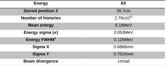
Table 1 - Parameters of the generated phase space for the segment s1. ... 55

Table 2 - Passing rates obtained in the gamma analysis between simulated and measured PDDs and transverse profiles at the considered depths. ... 74

Table 3 - Simulated transmission readings. ... 76

Table 4 - Determination of the transmission factor for the HD 120TM MLC. ... 76

Table 5 - Values used for the calculation of the DLG. ... 76

Table 6 - Passing rates obtained in the gamma analysis performed between the film and the calculated dose distributions for the IMRT plan. ... 82

Table 7 - Passing rates obtained in the gamma analysis performed between the portal image and the calculated dose distributions for the IMRT plan. ... 83

Table 8 - Gamma analysis results for the structures of interest. ... 85

Table 9 - Percentage of points passing the gamma criteria, considering the different dose distributions evaluated in VeriSoft® for the slice placed at -3.5cm from the isocenter marked in the phantom relatively to the z axis. ... 88

Table 10 - Percentage of points passing the gamma criteria, considering the different dose distributions evaluated in VeriSoft® for the slice placed at -6.25cm from the isocenter marked in the phantom relatively to the z axis. ... 90

Table 11 - Passing rates obtained in the gamma analysis for the different volumes of interest performed in PRIMO, not considering a positioning mismatch. ... 93

Table 12 - Passing rates obtained in the gamma analysis for the different volumes of interest performed in PRIMO, considering a positioning mismatch of +0.5cm in the x axis. ... 93

Table 13 - Passing rates for the situation without any positioning mismatch, considering the AAA algorithm. ... 95

Table 14 - Passing rates for the situation with a positioning mismatch of +0.5cm in the x axis, considering the AAA algorithm. ... 95

Table 15 - Passing rates for the situation without any positioning mismatch, considering the Acuros XB algorithm. ... 95

Table 16 - Passing rates for the situation with a positioning mismatch of +0.5cm in the x axis, considering the Acuros XB algorithm. ... 96

(12)

ix

List of Graphs

Graph 1 - Comparison between the measured and the calculated PDDs. ... 67 Graph 2 - Comparison between the measured and the calculated transverse profiles at

1.5cm depth. ... 68

Graph 3 - Comparison between the measured and the calculated transverse profiles at

5.0cm depth. ... 68

10.0cm depth. ... 69

20.0cm depth. ... 69

30.0cm depth. ... 69

each considered depth for a 2x2cm2 field size. ... 70

Graph 10 - Comparison between the measured and the calculated transverse profiles

at each considered depth for a 6x6cm2 field size. ... 71

Graph 17 - Plot of dose as function of MLC leaf gap. ... 77 Graph 18 - Dmin parameter assessed for the CTV and for the PTV considering the

various positioning mismatches simulated. The red line represents the 95% dose value. ... 100

(13)

x

Graph 19 - V95% parameter assessed for the CTV and for the PTV considering the

various positioning mismatches simulated. The red line represents the 95% dose value. ... 101

Graph 20 - Dose received by both kidneys for all the positioning shifts considered. The

(14)

xi

List of Figures

Figure 1 - Interactions of electrons with matter: (A) excitation, (B, C) ionization, (D)

bremsstrahlung (adapted from Gunderson, L. L. et al 2015). ... 5

Figure 2 - Bremsstrahlung and generation of characteristic x-rays (adapted from

Ahmed, S. N., 2015). ... 6

Figure 3 - Typical bremsstrahlung spectrum for an x-ray tube (adapted from Ahmed, S.

N., 2015). ... 6

Figure 4 - Regions of relative predominance for the three major interactions of photons

with an absorber medium. The left curve is the region where the cross sections for the photoelectric effect and Compton effect are equal (aτ = aσ). The right curve is the region

where the Compton cross section is identical to the pair production cross section (aσ

=aκ) (adapted from Sun, Y. et al, 2017). ... 8

Figure 5 - Schematic diagram of the photoelectric effect: hʋ is the energy of the

incident photon, EB is the shell binding energy and EK is the kinetic energy of the

ejected electron (adapted from Podgorsak, E. B., 2016). ... 9

Figure 6 - Schematic diagram of the Compton effect by a loosely bound electron

(adapted from Kharisov, B. I. et al, 2013). ... 10

Figure 7 - Schematic representation of pair production: (a) nuclear pair production in

the Coulomb field of the atomic nucleus; (b) electron pair production (triplet production) in the Coulomb field of an orbital electron (adapted from Podgorsak, E. B., 2016). ... 11

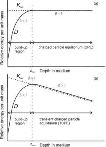
Figure 8 - Variation of the collision KERMA, , and absorbed dose, , with depth in

a medium, irradiated by a high-energy photon beam: (a) CPE; (b) Transient CPE. (adapted from Podgorsak, E. B., 2005). ... 16

Figure 9 - The working principle of the MLC (adapted from Romeijn, H. E. et al, 2005).

... 18

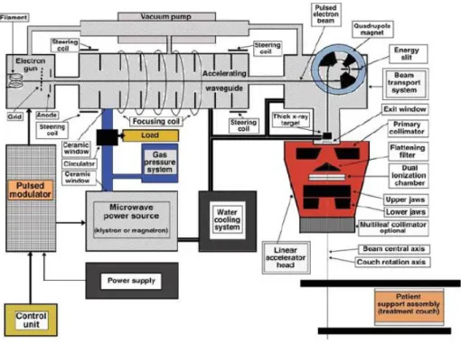
Figure 10 - The two banks of a Varian MLC (adapted from Hughes, J. L., 2013). ... 19 Figure 11 - General structure of a LINAC (adapted from Hamza-Lup, F. G., et al,

2014). ... 19

Figure 12 - Schematic block diagram of a LINAC (adapted from Podgorsak, E. B.,

2010). ... 19

Figure 13 - Transverse beam profile of a 10 MV flattened (dashed line) and unflattened

(solid line) photon beam (adapted from Prendergast, B. M. et al, 2013) ... 21

Figure 14 - Transverse profiles for : (a) 6MV FFF; (b) 10MV FFF photon beams; at

(15)

xii

Figure 15 - Example of a water tank phantom (adapted from Prezado, Y., et al, 2010).

... 23

Figure 16 - (a) Front view of RANDO phantom; (b) CT scan of the RANDO phantom

(adapted from Puchalska M. et al, 2014). ... 23

Figure 17 - Computational male and female phantoms (adapted from Xu, G. X, 2014).

... 24

Figure 18 - Percentage depth dose definition (adapted from Khan, F. M, 2014). ... 24 Figure 19 - Percentage depth doses for: (a) electron beams ranging from 6–20 MeV

for a field size of 10x10 cm2; (b) megavoltage x-ray beams ranging from 1·17–1·33 MeV (60Co) to 22 MV (adapted from Dicker, A. P., 2003, SSD not mentioned in the article, as well as the field size for photons). ... 25

Figure 20 - Flattened 6MV beam profile for a 5x5 cm2 field (adapted from Kuppusamy, T., 2017). ... 27

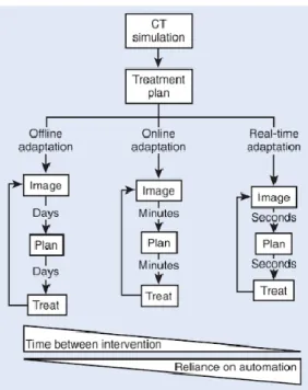
Figure 21 - The various adaption methods for radiotherapy and the required time and

automation associated (Hoppe, R. et al, 2010). ... 37

Figure 22 - 3D grid of cubic voxels used to segment a given geometry (adapted from

Bottigli, U. et al, 2004). ... 42

Figure 23 - Schematic diagram representing the layered structure of the simulation

engine based on PENELOPE 2011 provided by PRIMO (adapted from Rodriguez, M.

et al, 2013). ... 44 Figure 24 - Representation of the roud-leaf-end effect (adapted from Shende, R. et al,

2017). ... 58

Figure 25 - The 1cm gap defined by the HD 120TM MLC. ... 59

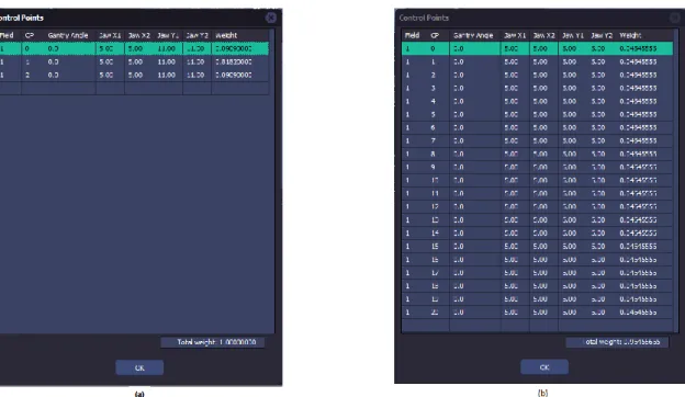
Figure 26 - (a) Control points of the plan as exported by the TPS; (b) Control points

after the edition of the project file. ... 59

Figure 27 - The RUPERT phantom used. ... 60 Figure 28 - (a) coordinate system defined in the TPS (EclipseTM); (b) coordinate system defined in PRIMO. ... 61

Figure 29 - CT illustrating the isocenter markers placed in the RUPERT phantom. .... 62 Figure 30 - The brain VMAT plan after its import to PRIMO. ... 62 Figure 31 - The simulated abdominal VMAT plan without positioning mismatch. ... 63 Figure 32 - Analysis of the generated phase space for the segment s1 (electrons are

represented by the blue curve, photons are represented by the red curve, and positrons are represented by the green curve). ... 65

Figure 33 - Profiles of the spatial distribution of (a) photons and (b) photons energy, in

(16)

xiii

Figure 34 - Surfaces representing (a) spatial distribution of photons and (b) spatial

distribution of photons energy, in the phase space created. ... 66

Figure 35 - (a) Gamma analysis performed on PRIMO for the PDD of a 10x10cm2 field;

(b) Gamma analysis performed on PRIMO for the transverse profile of a 10x10cm2 field at 1.5cm depth. ... 75

Figure 36 - (a) Dose distribution calculated by PRIMO. At the top of the image the

dose profiles taken along the axial, sagittal, and coronal directions of the orthogonal planes relative to point selected in the views, which is the isocenter in this case, are represented. Below it is illustrated the dose profile on the x axis at the isocenter plane (left) and a 3D view of the calculated dose distribution (right); (b) Gamma analysis between the PRIMO and TPS dose calculations performed on PRIMO. The voxels that pass the criteria are represented in blue and those that fail the criteria are indicated in red. The curves below represent the comparison of the transverse dose profile on the z axis between the PRIMO (blue) and the RP file (red) dose distributions at the isocenter. ... 79

Figure 37 - (a) Dose distribution obtained after the addition of control points to the .ppj

file; (b) Gamma analysis between the PRIMO and TPS calculation, performed on PRIMO. ... 81

Figure 38 - 2D gamma analysis performed between the film and the TPS calculation.

... 82

Figure 39 - 2D gamma analysis performed between the portal image and the TPS

calculation. ... 83

Figure 40 - Number of control points associated with the brain VMAT plan simulated in

PRIMO. ... 85

Figure 41 - Example of a gamma analysis for the PTV performed in PRIMO. The grey

axes intersection represents the isocenter ... 85

Figure 42 - Effect of the out of the body doses on the 2D gamma comparison

performed in VeriSoft® between the AAA calculation and the PRIMO simulation. ... 87

Figure 43 - 2D analysis, performed in VeriSoft®, between the TPS calculation and the PRIMO simulation after the removal of all the information outside of the body structure. ... 87

Figure 44 - Effect of the distance to the isocenter in the 2D gamma analysis results. In

the bottom image the isodose lines for the PRIMO calculation are represented. ... 89

Figure 45 - Result of the gamma analysis only considering the region of the distribution

(17)

xiv

Figure 46 - Radiochromic film placing in the RUPERT phantom (adapted from

Ghareeb, F. et al, 2017). ... 90

Figure 47 - Film boundary interpreted as dose in VeriSoft®. ... 90

Figure 48 - Intersection of two grey axes in the sagittal view representing the

localization of the films placed at (a) -3.5cm and at (b) -6.25, from the isocenter marked in the phantom relatively to the z axis. The red curve represents the PTV. .... 92

Figure 49 - Example of a gamma analysis of the PTV (red curve) performed in PRIMO

for the situation without a positioning mismatch, considering the simulation and the AAA calculation. The grey axes intersection represents the isocenter. ... 94

Figure 50 - Intersection of two grey axes in the sagittal view representing the

localization of the films placed at (a) -3.75cm; (b) -1.25cm; (c) +1.25cm; (d) +3.75cm, from the isocenter marked in the phantom relatively to the z axis, for the case without positioning mismatch. The red curve represents the PTV and the blue curve corresponds to the CTV. ... 96

Figure 51 - Intersection of two grey axes in the coronal view representing the

localization of the films placed at (a) -3.75cm; (b) +3.75cm, from the from the isocenter marked in the phantom relatively to the z axis, for the case without positioning mismatch. The red curve represents the PTV. ... 97

Figure 52 - Red square indicating the region of the films chosen for all the gamma

analysis performed in this study. ... 97

Figure 53 - DVHs comparison for the reference (PRIMO calculation) and external (AAA

calculation) dose distributions, relative to the various volumes of interest for a single treatment fraction without positioning mismatch. ... 99

(18)

xv

List of Abbreviations

3DCRT Three-Dimensional Conformal Radiation Therapy

AAA Analytical Anisotropic Algorithm

AAPM American Association of Physicists in Medicine

BEV Beam’s Eye View

CBCT Cone Beam Computed Tomography

CPE Charged Particle Equilibrium

CT Computed Tomography

CTV Clinical Target Volume

DICOM Digital Imaging and Communications in Medicine

DTA Distance To Agreement

DLG Dosimetric Leaf Gap

DVH Dose-Volume Histogram

eV Electron Volt

FF Flattening Filter

FFF Flatenning Filter Free

FWHM Full Width at Half Maximum

GTV Gross Tumour Volume

(19)

xvi

ICRU International Commission on Radiation Units and Measurements

IMRT Intensity Modulated Radiation Therapy

IGRT Image-Guided Radiotherapy

ITV Internal Target Volume

IPOPFG Instituto Português de Oncologia de Francisco Gentil

KERMA Kinetic energy released in matter

LASER Light Amplification by Stimulated Emission of Radiation

LCG Linear Congruential Generator

LINAC Linear Accelerator

MATLAB Matrix Laboratory

MC Monte Carlo

MLC Multileaf Collimator

MeV Mega-Electron Volt

MOSFET Metal-Oxide-Semiconductor Field-Effect Transistor

MU Monitor Unit

MV Megavolt

PDD Percentage Depth Dose

(20)

xvii

PTV Planning Target Volume

OAR Organ at Risk

QA Quality Assurance

QUANTEC Quantitative Analysis of Normal Tissue Effects in the Clinic

RNG Random Number Generator

RT External Beam Radiotherapy

SRS Stereotactic Radiosurgery

SRT Stereotactic Radiotherapy

SSD Source-Surface Distance

TCP Tumour Control Probability

TPS Treatment Planning System

VMAT Volumetric Modulated Arc Therapy

(21)

1

1.) Introduction

1.1. ) Motivation

In External Beam Radiotherapy (RT) the idea of modulating the radiation field through the motion of a collimating system developed into the Intensity Modulated Radiation Therapy (IMRT) concept. IMRT allows to achieve a practical clinical gain by the creation of complex dose distribution patterns, at the price of great complexity. Volumetric Modulated Arc Therapy (VMAT) is a generalization of the IMRT technique, which introduces the dynamic rotation of the gantry during the treatment.

The patient position is one of the most critical steps during the RT process. A mismatch in the clinical setup can produce undesirable effects from the dosimetric point of view. In principle, the effect of the positioning uncertainty cannot be predictable as it depends on several factors, such as the patient’s anatomy, the anatomical region to treat, the radiation beam energy, and the RT technique.

The increase of the technological complexity in VMAT requires patient dedicated Quality Assurance (QA) programs in order to ensure safety to the patient and treatment effectiveness. The pre-treatment patient-specific QA becomes more important as the treatment complexity increases. A general approach is to make use of QA dedicated phantoms and to recalculate the dose distribution substituting the patient with the phantom. Delivering the planned VMAT radiation beam on the phantom allows a comparison between the dose distribution calculated by the Treatment Planning System (TPS) and the measurement. The most common tool to assess the equivalence between the TPS calculated and the measured (2D/3D) dose distribution is the gamma index.

The delivery of the VMAT radiation beam on the phantom requires that the positioning tools, at the treatment unit, are perfectly calibrated and allow the phantom to be placed with the minimum operator uncertainty. In principle, the positioning of patient and phantom can follow the same process. If a mismatch in the positioning instruments occurs, the QA can provide unexpected false results.

In Medical Physics, several dosimetric problems have been addressed by means of the Monte Carlo (MC) simulation method. The MC approach is considered the gold standard method for radiation transport simulation. In some cases it is the only one to perform accurate absorbed dose calculations, since it provides the most detailed and complete description of the radiation fields and the particle transport in matter.

(22)

2

The MC method can be a powerful tool to evaluate dose distributions in undesirable, but possible, conditions, such as patient and/or phantom positioning mismatch. Several codes are available for MC simulations in the field of RT, some of which are GEANT4, EGSnrc/BEAMnrc, PENELOPE, FLUKA, and MCNP. Recently, a new MC code named PRIMO that makes use of the PENELOPE features was developed.

The PRIMO simulation software has a user-friendly approach, which is a suitable and competitive characteristic for the clinical activity. Among the different linear accelerator (LINAC) models provided in the PRIMO release, Varian FakeBeam is an available model of the Varian TrueBeamTM unit. TrueBeamTM has very peculiar features such as the absence of the flattening filter (FFF – Flattening Filter Free), respiratory gating, and a real-time tracking system. This particular LINAC can be used for a wide range of RT applications, including stereotactic and VMAT techniques.

A version of PRIMO is installed at Instituto Português de Oncologia do Porto de Francisco Gentil (IPOPFG) and previous experience on radiation beam modeling of a TrueBeamTM unit has been developed (Master’s Degree thesis on implementation of VMAT MC simulation in the clinical activity). As a result, adequate conditions were established for the realization of this thesis.

1.2.) Thesis Outline

This thesis is divided into seven chapters. In chapter one the framework of the work is introduced. Then, chapter two includes the theoretical and experimental background associated with radiation therapy and Monte Carlo simulations. Chapter three represents the objectives of the work performed. Flowingly, in chapter four the materials and methods used are mentioned. Afterwards, chapter five includes all the results obtained and their discussion. Next, chapter six contains the protocol developed for the adaption of the treatment plan. In chapter seven the conclusions of this work are withdrawn and finally chapter eight encompasses the bibliography used.

(23)

3

2.) Theoretical and Experimental

Background

Cancer is one of the main life-threatening diseases worldwide and it is expected a rise in this public health problem due to multiple reasons, such as the increase of the Human life expectancy, the continuous growth of the population, and the obesity upsurge (Global Burden of Disease Cancer Collaboration, 2017; Jung, K. et al, 2017).

Some oncological therapies currently used are surgery, chemotherapy, radiation therapy (radiotherapy), immunotherapy, hormone therapy, and targeted therapy. Frequently, cancer’s therapeutic approach involves a combination of local therapy, like surgery and/or radiotherapy, and systemic therapy, such as chemotherapy and/or hormone therapy (Liu, K. et al, 2017; Silverman, P., 2012).

Radiotherapy consists in the use of ionizing radiation to damage the tumorous cells’ DNA, leading to the shrinkage and possibly to the control of solid tumours. Commonly, this area is further divided in external beam radiotherapy and brachytherapy. In this thesis the focus will be on external beam radiotherapy, where an ionizing radiation source, placed at some distance from the individual, produces a beam of high energy photons, neutrons or charged particles. The beam is then directed to a specific region of the patient’s body in order to deliver a therapeutic amount of radiation, usually referred as radiation dose or simply dose, to a target volume (Salvajoli, J. V. et al, 2008; Silver, J., 2006; Voutilainen, A. 2016).

2.1.) Radiobiological Background

Ionizing radiation can damage the cells’ DNA directly (direct action) or interact with water molecules and produce free radicals that react with this biological entity, a process known as indirect action. A single strand break, as well as spatially distant multiple single strand breaks, is likely to be repaired by the cell. On the other hand, when two opposite or very close breaks occur there is a high probability of a double strand break, which is considered to be the main reason for radiation induced cell death (Baskar, R. et al, 2014; Voutilainen, A. 2016). Ionizing radiation causes similar harm in normal and tumorous cells, however experimental results show that healthy cells can repair the DNA damage faster than cancerous cells. This factor combined with other effects, like reoxygenation of neoplastic cells and reassortment of cells during the cell cycle, leads to an increased sensitivity of the cancerous cells to radiation when the dose is delivered in small fractions over longer periods of time, instead of a

(24)

4

large fraction once. Nevertheless, there is a possibility of further complications for the patient because, for example, the healthy cells may not undergo apoptosis when they are not able to repair all the damage done to the DNA strand or after performing wrong corrections in that molecule (Baskar, R. et al, 2014; Voyant, C. et al, 2014).

2.2.) Radiation Physics

In this section, the physics associated with the interaction of electrons and photons with matter will be addressed. These are the two types of radiation that a linear accelerator can produce and, consequently, the only ones used at Instituto Português de Oncologia do Porto de Francisco Gentil (IPOPFG) for external radiotherapy treatments. Also, the basic quantities and units associated with radiation dosimetry will be briefly described.

2.2.1.) Interaction of Electrons with Matter

Since electrons have an electric charge, they experience Coulomb interactions with nuclei and atomic electrons during their passage through matter, therefore these particles are defined as directly ionizing radiation. In each interaction event there are several possible energy losses and angular changes that an electron can undergo (Mozumder, A. et al, 2003). Any momentum change of an incident particle is defined as a collision and it can be classified as (Autran, J. et al 2015; Podgorsak, E. B., 2016; Vidyasagar; P. B. et al, 2017; Zhang, S.-L., 2012):

 Elastic collision: the kinetic energy of the involved particles after and before the encounter is equal and the incident particle is just deflected from its original path; for energies above ~100 eV elastic collisions with atomic electrons can be neglected;

 Inelastic collision: kinetic energy is transferred to the struck particle (nucleus or atomic electron), as a result the involved particles do not have the same kinetic energy after and before the encounter, albeit the total energy is conserved in the process.

The major interaction processes of electrons with matter are excitation, ionization, and inelastic scattering by nuclei, which is known as bremsstrahlung (Sharma, S. 2008).

An incident electron can excite an atomic electron to a higher energy orbital when there is an inelastic collision between the two particles (figure 1.A) and, if the energy provided to the orbital electron is high enough, it may result in the ejection of

(25)

5

the struck electron, leading to the ionization of the atom. The energy of the emitted electron depends on its binding energy as well as on the incident electron’s energy. When the ejected electron leaves the atom a vacancy in the electronic band structure is created, which must be filled for the atom to reach its lowest energy state (except when the ejection occurs at the outer shell - figure 1.B and 1.C). If the expelled electron is from an inner shell of the atom, the filling of the vacancy left behind, by the transition of another electron located in a higher energy orbital, originates a release of energy equal to the binding energy difference between the two orbital levels involved (Hornyak, G.L. et al, 2008; Knapp, F.F.R. et al 2016; Leroy, C. 2016). This energy can be emitted via a photon (radiative emission – characteristic x-rays) or be absorbed by a bound electron of a higher shell, causing its ejection (this released electron is called Auger electron). The probability of non-radiative transitions, with consequent emission of Auger electrons, is higher for low atomic number materials (Splinter, R. 2016).

Figure 1 - Interactions of electrons with matter: (A) excitation, (B, C) ionization, (D) bremsstrahlung (adapted from Gunderson, L. L. et al 2015).

Another important interaction of electrons with matter is bremsstrahlung (braking radiation – figure 1.D). This process is characterized by the electromagnetic radiation emitted per charged particles when they decelerate in a medium, due to the inelastic interaction with nuclei of absorber atoms within matter. Bremsstrahlung is the dominant mode through which the moderate to high energy electrons lose energy in high atomic number materials (Bushong, S. C., 2017; Halperin, E. C. et al, 2013; Podgorsak, E. B., 2016). For the energies used in external radiotherapy, in the order of MeVs, this interaction produces a continuous x-ray emission spectrum, for the reason that there are no transitions between quantized energy levels involved in the process

(26)

6

as opposed to characteristic x-rays, where there exists a well-defined transition that leads to a discrete x-ray emission spectrum (Halperin, E. C. et al, 2013).

Figure 2 - Bremsstrahlung and generation of characteristic x-rays (adapted from Ahmed, S. N., 2015).

Nevertheless, the bremsstrahlung continuous emission spectrum frequently includes single strong peaks, because the bombarding electrons can expel electrons from the inner atomic shells of the struck particle. As a result, the filling of these vacancies by other electrons located in the higher energy orbitals, as discussed before, produces characteristic x-rays or Auger electrons (Johnston J. et al, 2015).

Figure 3 - Typical bremsstrahlung spectrum for an x-ray tube (adapted from Ahmed, S. N., 2015).

There are other types of elastic interactions of electrons with matter, such as Møller scattering and Bhabha scattering, but for the energy range used in radiotherapy this processes can be neglected (Podgorsak, E. B., 2016).

2.2.2.) Interaction of Photons with Matter

Photons are quanta of electromagnetic field, which interact with matter in a different way than electrons due to their charge neutrality, being classified as indirectly

(27)

7

ionizing radiation because they deposit energy in an absorbing medium through a two-step process (Krems, R. V., 2018; Nikjoo, H. et al, 2012; Podgorsak, E. B., 2016):

 First step: energy transfer from the photon to an energetic charged particle with low weight (electron or positron) that is released in the medium;

 Second step: deposition of energy in the medium by the released low weight charged particle.

In radiotherapy treatments, photon beams are directed towards the patient’s body. As they pass through the individual, there are three possible outcomes for each photon (Nikjoo, H. et al, 2012). It can:

 Pass through the patient without interacting;

 Interact with the patient and be completely absorbed, depositing its total energy in the medium;

 Interact with the patient, deposit part of its energy in the medium, and experience scattering or deflection from its original direction.

There are various interactions that each photon can undergo: it may interact with an atom as a whole, with the nucleus of an atom, or with an orbital electron of the atom. Therefore, different photons in a given beam passing through a certain medium do not necessarily interact in an identical way with matter as they travel. The occurrence probability associated to a particular interaction is generally expressed in terms of an interaction cross section, which depends on the photon’s energy as well as on the density and atomic number of the absorber material (Dössel, O. et al, 2010; Key, T., 2013; Podgorsak, E. B., 2016). The cross section for a given interaction can be defined as the area of the target (atomic nucleus or subatomic particle) perpendicular to the direction of the incident photon beam; the event occurs whenever a particle hits this area (Brahme, A. et al, 2014; Podgorsak, E. B., 2016).

The three main interactions of photons with matter, for the energy range used in radiotherapy, are: the photoelectric effect, the Compton effect, and the pair production. They are dominant at different energies and for different absorber atomic number values, as it is possible to see in figure 4 (Podgorsak, E. B., 2016).

(28)

8

Figure 4 - Regions of relative predominance for the three major interactions of photons with an absorber medium. The left curve is the region where the cross sections for the photoelectric effect and Compton effect are equal (aτ = aσ). The

right curve is the region where the Compton cross section is identical to the pair production cross section (aσ =aκ)

(adapted from Sun, Y. et al, 2017).

These processes (figure 4) are classified as inelastic because the involved particles do not have the same kinetic energy before and after the event (Biersack, H.-J. et al, 2007). Additionally, there are two elastic interactions of photons with matter relevant to medical physics (not shown in figure 4), namely Thomson scattering and Rayleigh scattering (Cremer, J. T. 2012). The latter is considered elastic, even though the atom as a whole absorbs the transferred momentum, for the reason that the recoil energy is very small and, therefore, the scattered photon has essentially the same energy as the original photon (Podgorsak, E. B., 2016). These two processes occur mainly for low energy photons and they do not originate a considerable energy deposition in the medium. Since external beam radiotherapy relies on the energy transfer to a precise location of the patients’ body, these elastic interactions will not be detailed in this thesis (Barazzuol, L. et al, 2012; Podgorsak, E. B., 2016; Turner, J. E., 2007).

As it is possible to see from figure 4, the photoelectric effect is dominant for photons in the energy range of 0.01 MeV to ~0.1 MeV and its prevalence upsurges with the increase of the absorber’s atomic number (Z) (Chin, L. S. et al, 2015). During this process an incident photon is completely absorbed by the medium and an electron from a shell of the struck atom is ejected (known as “photoelectron”). The considerations of conservation of energy and momentum indicate that this interaction can only occur on a tightly bound (shell with a higher binding energy) electron, rather than with a “free electron” (shell with a lower binding energy), so that the atom can pick

(29)

9

up the difference of momentum and energy between the photon and the photoelectron (Chin, L. S. et al, 2015; Brahme, A. et al, 2014; Yang, F. et al, 2010).

Figure 5 - Schematic diagram of the photoelectric effect: hʋ is the energy of the incident photon, EB is the shell binding

energy and EK is the kinetic energy of the ejected electron (adapted from Podgorsak, E. B., 2016).

From figure 5, it is possible to conclude that the energy of the incident photon must be superior to the electron’s binding energy for the photoelectron to be ejected. As a result, the energy of the emitted particle is equal to the incident photon energy minus the binding energy of the ejected orbital electron. In this interaction the atom is left in an ionized state (Saha, G. B., 2013). Sometimes the photon energy is not high enough to emit an orbital electron, but it is sufficient to raise it to a higher energy orbital, leaving the atom in an excited state (Müller, M., 2007). When an ionization of an atom occurs, the filling of the vacancy left behind is similar to the process described in section 2.2.1.), also occurring the emission of an Auger electron or a characteristic x-ray photon (Klockenkämper, R. et al, 2014).

An important last note about this interaction is that the angular distribution of the ejected electrons is determined by the incident photon energy. At low photon energies the photoelectrons tend to be ejected at ~90º relatively to the incident photon direction and, as the photon energy increases, the emission angle starts to decrease. Consequently the orientation of the electron emission progressively changes towards the same direction as that of the incident photon (Green, D., 2014; Podgorsak, E. B., 2016).

A different interaction starts dominating over the photoelectric effect when the energy of the incident photon increases (figure 4). In this process, called Compton effect, or scattering, the photon interacts with a free or loosely bound orbital electron, so that it is possible to consider it stationary for the fact that its binding energy is insignificant in comparison to the photon’s energy. Two particles result from this interaction: a scattered photon with lower energy than the incident photon, and an

(30)

10

electron known as Compton electron, which is ejected from the atom with a certain kinetic energy (Bushong, S. C., 2017; Kharisov, B. I. et al, 2013; McParland, B. J., 2010). The Compton effect may also occur between a photon and a nucleus, however this specific process can be neglected in the area of medical physics and radiation dosimetry (Podgorsak, E. B., 2016).

Figure 6 - Schematic diagram of the Compton effect by a loosely bound electron (adapted from Kharisov, B. I. et al, 2013).

From the analysis of figure 4, it is possible to view that the pair production processes begin to dominate over the Compton effect as the incident photon energy is further increased and the atomic number of the absorber rises (dependence ~Z2). When the incident photon energy, , surpasses ~1.02MeV, i.e. twice the electron’s rest mass ( ), the production of an electron-positron pair in combination with the complete absorption of the incident photon becomes energetically viable (Leroy, C., 2012; Pawlicki, T. et al, 2016). Three quantities must be conserved for the occurrence of this interaction: energy, charge, and momentum. If the photon’s energy verifies the condition stated before ( ), energy and charge can be conserved even if pair production befalls in free space. However, the conservation of its linear momentum implies that this phenomenon can only occur in the Coulomb field of another particle (collision partner). When the collision partner is an atomic nucleus, an appropriate portion of the momentum carried by the incident photon is taken up by that structure (figure 7(a)) (Henley, E. M., 2007; Podgorsak, E. B., 2016; Thornton, S. T. et al, 2013). Otherwise, if , an orbital electron can receive the exceeding linear momentum. The recoil energy of this atomic electron might be substantial and the process is known as triplet production (pair production in the Coulomb field of the electron). When such event occurs, three particles leave the site of interaction (figure 7(b)) (Andreo, P. et al 2017; Pawlicki, T. et al, 2016).

(31)

11

Figure 7 - Schematic representation of pair production: (a) nuclear pair production in the Coulomb field of the atomic nucleus; (b) electron pair production (triplet production) in the Coulomb field of an orbital electron (adapted from Podgorsak, E. B., 2016).

The positron resulting from this interaction moves through an absorbing medium and, therefore, experiences kinetic energy losses by collisional and radiative processes via Coulomb interactions with orbital electrons and nuclei of the absorber (Podgorsak, E. B., 2016). When the energy of this particle becomes sufficiently low, it experiences a process of annihilation with an orbital electron of the absorber, yielding two photons that approximately move in opposite directions (~180º) (Herrmann, K. et al, 2016; Niederhuber, J. E. et al, 2013; Podgorsak, E. B., 2016):

Another possible interaction between an energetic photon (8-16 MeV) and an absorber nucleus is the photonuclear reaction (also called photodisintegration), in which the atomic nucleus absorbs a photon. The most probable outcome of such process is the emission of a single neutron. This process does not play a role in overall photon attenuation studies, but it is important in shielding calculations whenever the energy of the photons exceeds the photonuclear reaction threshold (Chang, D. et al, 2014; Johnson, T. E., 2017; Podgorsak, E. B., 2016).

2.2.2.1.) Photon Attenuation Coefficients

The interaction mechanisms described before do not occur singly, but rather they combine to produce a global attenuation of the photon beam as it passes through matter. Attenuation can be interpreted as the removal of photons from the original photon beam and it is governed by the inverse-square law, along with absorption and scattering events. This weakening of the beam is frequently expressed in terms of an attenuation coefficient, which describes the interaction probability of the photons in a material. Generally, the macroscopic attenuation coefficient is given by the sum of the attenuation coefficients for all the possible interactions that a photon, with a given energy, can have with an absorber medium (Ahmed, S. N., 2015; Bushberg, J. T. et al,

(32)

12

2011; Huda, W; 2010; Podgorsak, E. B., 2016; Singh, H. et al, 2016; Vosper, M. et al, 2011).

2.2.3.) Basic Quantities and Units in Radiation Dosimetry

In radiotherapy, the prescribed dose must be delivered accurately and safely to the target site in order to reach the treatment goal and, simultaneously, minimize the probability of complications in normal tissues (Lee, E. K. et al, 2017). Therefore, the precise measurement of the deposited energy is fundamental for the medical use of radiation (van der Merwe, D. et al, 2017). In such context, dosimetry appears as the measurement, calculation, and assessment of the dose delivered to a given volume (Adlienė, R. et al, 2017; Meghzifene, A., et al¸ 2010; Tweedy, J. T., 2013).

This area can be divided into two categories, namely absolute dosimetry and relative dosimetry. Absolute dosimetry consists in a direct measure of the absorbed dose, or another dose related quantity, at a certain point by a dosimeter (section 2.5.1.)) under standard conditions, not needing a calibration of the measurement device in a known radiation field. On the other hand, relative dosimetry involves dosimeters that require a calibration of their response to ionizing radiation, in a well-defined radiation field, before the radiation induced signal can be used to obtain dosimetric information (Podgorsak, E. B., 2005; Podgorsak, E. B., 2016; Watanabe, Y., 2014).

There are numerous quantities that were introduced with the objective of quantifying radiation. In this thesis, only the most important will be addressed, according to the International Commission on Radiation Units and Measurements (ICRU) report No.85.

2.2.3.1.) Particle Number and Radiant Energy

The particle number, N, is the number of particles that are emitted, transferred or received. SI Unit: dimensionless.

The radiant energy, R, is the energy (excluding rest energy) of the particles that are emitted, transferred or received. SI Unit: J.

2.2.3.2.) Flux and Energy Flux

The flux, ̇, is the increase of the particle number ( ) per time interval ( ), thus:

(33)

13 ̇

SI Unit: s-1.

The energy flux, ̇, is the increase of radiant energy ( ) per time interval , thus:

̇ SI Unit: W.

2.2.3.3.) Fluence and Energy Fluence

The fluence, , is the number of particles ( ) incident on a sphere of

cross-sectional area da, thus

SI Unit: m-2.

The energy fluence, , is the radiant energy ( ) incident on a sphere of

cross-sectional area , thus

SI Unit: J m-2

2.2.3.4.) Fluence Rate and Energy-Fluence Rate

The fluence rate, ̇, is the fluence increase ( ) per time interval , thus: ̇

SI Unit: m-2 s-1

The energy-fluence rate, ̇, is the increase of the energy fluence in the time interval dt, thus:

̇ SI Unit: W m-2.

2.2.3.5.) KERMA

According to Podgorsak, E. B., 2016, KERMA is an acronym for “Kinetic energy released in matter” and it is only defined for indirectly ionizing radiation. ICRU report No. 85 describes this quantity as: the quotient of by , where is the mean

sum of the initial kinetic energies of all the charged particles liberated in a mass of

a material by the uncharged particles incident on , thus

(1) (2) (3) (4) (5) (6)

(34)

14

(7)

SI Unit: J Kg-1 = Gy.

The released charged particles can lose kinetic energy through inelastic collisions with atomic electrons (ionization and excitation) or by radiative processes involving atomic nuclei. Therefore KERMA can be decomposed in two quantities, the collision KERMA, which does not take into account the radiative losses of the liberated charged particles, and the radiation KERMA, , that only considers the energy emitted through radiative processes, thus (Khan, F. M. et al, 2014; Nilson, B. N., 2015):

For low atomic number materials (e.g., air, water, soft tissue), charged particles lose the major part of their kinetic energy via collision interactions and only a small fraction through emission of radiation. increases with increasing particle energy, however for absorbed dose (2.2.3.6.)) calculations the radiative losses are not considered because the emitted radiation can exit from the volume of interest. As a result, only the collision KERMA is used as an estimate of the absorbed dose, in conditions of charged particle equilibrium (CPE) (2.2.3.6.1.)) (Khan, F. M. et al, 2014; Yukihara, E. G. et al, 2010).

2.2.3.6.) Absorbed Dose

The absorbed dose, , is the mean energy imparted by ionizing radiation ̅ to

matter of mass , thus

̅ SI Unit: J Kg-1 = Gy.

This quantity is defined for all types of ionizing radiation (i.e., directly and indirectly ionizing radiation), all materials, and all energies, whereas KERMA is only defined for indirectly ionizing radiation (Khan, F. M. et al, 2014). As discussed in section 2.2.3.5.1.), the absorbed dose can be estimated by the collisional KERMA in conditions of CPE.

A relevant quantity related to the absorbed dose is the equivalent dose, defined as the absorbed dose multiplied by a radiation weighting factor(SI Unit: Sievert (Sv)). This measure considers the biological effectiveness of radiation, i.e. the effectiveness of a given type of radiation in causing damage to tissues and organs, and it depends on the radiation type and energy (Hoskin, P. et al, 2011; Symonds, R. P. et al, 2012). Another pertinent quantity associated with absorbed dose is the effective dose, which

(8)

(35)

15

is defined as the tissue-weighted sum of the equivalent doses associated with all the tissues and organs exposed to ionizing radiation (SI unit: Sievert (Sv)). In this case, the weighting factor is called tissue weighting factor and it assesses the risk of stochastic effects that may result from an irradiation of that particular tissue. Therefore, the effective dose evaluates the stochastic health risk to the whole body resulting from a given radiation dose (Allen, B. et al, 2012; Hoskin, P. et al, 2011).

2.2.3.6.1.) Charged Particle Equilibrium (CPE)

Charged particle equilibrium (CPE), or electronic equilibrium, is said to exist in a volume if each charged particle of a given type, direction, and energy exiting from that volume is replaced by a particle of equal type, direction, and energy entering the same volume (Attix, F. H., 2008). When CPE conditions are fulfilled it is valid to assume that the collision KERMA is equal to the absorbed dose (2.2.3.6.)) (Sibtain, A. et al, 2012).

In the buildup region the CPE requirements are not verified, consequently the deposited energy cannot be inferred from the energy transfer to matter in this location. From figure 8(a), it is possible to see that immediately beneath the patient’s surface the absorbed dose ( ) is much smaller than the collision KERMA ( ). However, increases quickly with depth (z) until CPE is achieved at zmax (depth of maximum

absorbed dose) and both quantities become comparable (Andreo, P. et al, 2017; Attix, F. H., 2008; Das, I. J., 2017; Nilson, B. N., 2015).

The difference between absorbed dose and collision KERMA, observed in the buildup region, occurs due to the relative long range of the energetic secondary charged particles (electrons and positrons). When these particles are released by interactions of photons with matter they travel through matter, depositing their energy in the medium at a given distance from the location where they were initially freed (Ghom, A. G., 2016).

Considering a more realistic case (figure 8(b)), beyond zmax both dose and

collision KERMA decrease due to the photon attenuation in the medium, resulting in a transient rather than a true CPE. In this situation, the energy entering the volume is slightly larger than the energy leaving that same volume and the absorbed dose is proportional, but not equal, to the collision KERMA (Andreo, P. et al, 2017; Attix, F. H., 2008; Das, I. J., 2017; Nilson, B. N., 2015).

(36)

16

Figure 8 - Variation of the collision KERMA, , and absorbed dose, , with depth in a medium, irradiated by a high-energy photon beam: (a) CPE; (b) Transient CPE.

(adapted from Podgorsak, E. B., 2005).

2.2.3.7.) Exposure (X)

Exposure, , is defined as: the quotient of by , where is the absolute

value of the mean total charge of the ions of one sign produced when all the electrons

and positrons liberated or created by photons incident on a mass of dry air are

completely stopped in dry air, thus:

SI Unit: C kg-1.

Summing up, this quantity is only defined for photons and it characterizes the capability of photons to ionize the air.

An alternative unit to this measure is the roentgen (R) and it is defined as the amount of photon radiation needed to produce a charge of 2.54x10-4 C per kilogram of dry air (under standard conditions for pressure and temperature) (Haynes, K. et al, 2013).

(37)

17

2.3.) The Linear Accelerator

The key equipment in external beam radiotherapy is the linear accelerator (LINAC), figures 11 and 12, because it is the source of the ionizing radiation beams used for patient treatment (Healy, B. J. et al, 2016).

The primary source of radiation in the LINAC is the electron gun. This component of the accelerator has a heated tungsten filament which, through thermionic emission, emits electrons that will form the LINAC beam (Bhattacharjee et al, 2012; Chin, L. S., 2012; Symonds, R. P. et al, 2012). After the emission, the electrons are accelerated in a waveguide by means of electromagnetic waves in the microwave range, which are generated via a magnetron or a klystron (Cherry, P. et al, 2009; Hanna, S., 2012; Hoppe, R. et al, 2010; Symonds, R. P. et al, 2012). For LINACs that produce electron beams of 6MV or higher, the necessary accelerating waveguide length is too long to sit in line with the target and so it becomes useful to bend the electron beam through the use of bending magnets. The most commonly used bending systems are named according to the angle that electrons are turned, namely: the 90º bending, 270º bending, and the slalom system (also called 112.5º bending) in which the electrons take a zigzag path (Cherry, P. et al, 2009; Khan, F. M., 2012; Kuppusamy, T., 2017).

The electrons that exit the bending magnets system can be used directly for treatment on the body’s surface, or they can collide with a target, producing high energy x-rays through bremsstrahlung that can be used to treat deeper areas within the patient (Rahbar, R. et al, 2013; Snider, J. W. et al, 2016). The resulting beam passes through a primary collimator, where it is collimated. This component is a conical opening machined in a block of a shielding material and it defines the maximum circular field (Cherry, P. et al, 2009; Podgorsak, E. B., 2005).

In the clinical energy range (4MV – 25MV) the angular distribution of the bremsstrahlung photons is preferentially in the direction of the incident electrons that exit from the bending magnets system, creating a forward peaked (bell-shaped) transverse dose profile (figure 11). Therefore, in order to provide a flat (uniform) dose distribution at a defined depth, a flattening filter (FF) is introduced in the beam path (Joiner, M. C. et al, 2009; Xiao, Y et al, 2015; Yan, Y. et al, 2016). This component has a conical shape in order to flatten the forward peaked bremsstrahlung spectrum of MV photons. The type of FF used depends on the beam energy produced by the LINAC (Podgorsak, E. B., 2005; Sharma, S. D., 2011; Xiao, Y et al, 2015).

Below the flattening filter there are dual, sealed, and independent, ionization chambers. These chambers are sealed in order to give a constant reading at a

(38)

18

constant dose rate, independently of the temperature and pressure in the bunker. Therefore, they can terminate the irradiation when the planned number of monitor units (MUs) is debited. The advantage of having a dual system is that if the primary chamber fails during the treatment, the secondary dose monitoring system can terminate the irradiation when the selected MUs are surpassed by a set limit, providing additional safety for the patient by preventing an excessive output of radiation (Cherry, P. et al, 2009; Washington, C. M. et al, 2015).

Afterwards, the collimated beam is truncated by the secondary collimators, also known as jaws. These consist of two pairs of adjustable blocks, made of a high Z material (e.g., tungsten or lead) and perpendicular between them. The jaws restrict the radiation emerging from the LINAC’s head to specific square or rectangular fields, ranging from 1x1 cm2 to 40x40 cm2 at the isocenter of the accelerator (Cherry, P. et al, 2009; Podgorsak, E. B., 2012; Sikora, M. P., 2011). The isocenter is the point where the rotation axes of the treatment couch, the gantry, and the collimator intersect (Khan, F. M. et al, 2014; Voutilainen, A. 2016). Most modern models of LINACs have an additional system for beam collimation called the multileaf collimator (MLC), figure 9. This component is made up by several thin leaves of a high atomic number material (typically tungsten), allowing the dynamic design of practically any field shape for patient irradiation (Goh, G. et al, 2015; Jeraj, M. et al, 2004; Salles A. A. F. et al, 2011). The MLC is divided into two carriages, also called bank A and bank B, each of which with half of the total number of MLC leaves (figure 10) (Hughes, J. L., 2013). Nowadays, the MLCs used in the clinical practice may have 40 till 160 leaves. These leaves can have different widths, ranging from some millimeters until 1 cm. Every leaf is computer controlled, allowing field conformations with accuracy better than 1mm (Best, L. et al, 2013; Chin, L. S. et al, 2015; Jeraj, M. et al, 2004; Klüter, S. et al, 2009; Orlandini, L. C. et al, 2015).

(39)

19

Figure 10 - The two banks of a Varian MLC (adapted from Hughes, J. L., 2013).

Figure 11 - General structure of a LINAC (adapted from Hamza-Lup, F. G., et al, 2014).