Lisboom, speculation in Lisbon’s housing market

LISBOOM,

SPECULATION IN LISBON’S

HOUSING MARKET

Carlos Bernardo Bento Costa

Dissertation presented as the partial requirement for

obtaining a Master's degree in Statistics and Information

Management

NOVA Information Management School

Instituto Superior de Estatística e Gestão de Informação

Universidade Nova de Lisboa

LISBOOM, SPECULATION IN LISBON’S

HOUSING MARKET

Carlos Bernardo Bento Costa

Dissertation presented as the partial requirement for obtaining a Master's degree in Statistics and Information Management Specialization in Risk Analysis and

Management

Advisor: Flávio Luís Portas Pinheiro

ACKNOWLEDGEMENTS

- My family, for always pushing me to be better no matter what.

- Daniela, for always being by my side.

- My advisor, Flávio, for the guidance, trust, and discussions provided

while working in this research.

- To brazilian jiu-jitsu as a martial art, which taught me that there isn’t

nothing you can’t overcome if you put your mind into it.

- Python, community and developers, which these recent years

contributed a lot to the way I problem solve and approach data problems.

ABSTRACT

A degree of speculation has always been present in the major asset markets worldwide and the real estate market is not exempt of it. During this research, focused exclusively on Lisbon’s housing market, we discovered that real estate evaluation has never experienced higher values, and currently, it is difficult to provide support to justify an increase of this magnitude, not only that, but there was never a time in which more real estate transactions were conducted in such small-timeframes, this is also due to the current cost of money as the rates provided by the Central European Bank have been negative in these recent years, making the cost of money considerably low, thus increasing purchasing power and, with this ease of access in getting a higher degree of purchasing power, the means investors have to invest in asset markets are widely increased, with this increase will come the opportunity of asset trading in much smaller timeframes, which will serve as base to speculation growth around housing market.

KEYWORDS

INDEX

1. Intro ... 1

2. Literature Review ... 4

2.1. Bubble Definition ... 4

2.2. Economic impact ... 5

2.3. Drivers for pricing variation ... 9

2.4. Market analysis techniques ... 12

2.4.1. Price-to-income Ratio ... 14

2.4.2. Price-to-rent Ratio ... 14

2.4.3. User Cost of Housing (Imputed Rent) ... 15

2.5. Feature overview ... 18

3. Methodology ... 19

3.1. Ratio Construction ... 21

3.2. Exploratory data analysis ... 22

3.3. A proxy for demand ... 24

4. Analysis and Results ... 26

4.1. Economic features ... 26

4.2. Prices, rental and buying markets ... 30

4.3. Cost benefit, interest rates, homeowning expenses ... 36

4.4. Tourism, short-term rental, online interest ... 39

4.5. A proxy for demand ... 42

4.6. Data limitations, area change ... 45

5. Conclusions ... 48

6. Limitations and further work ... 52

7. Bibliography ... 53

FIGURE INDEX

Figure 1: Portuguese GDP, EUR, source: World Bank ... 26

Figure 2: Portuguese GDP Growth, source: World Bank ... 26

Figure 3: Portuguese GDP per-capita growth, source: World Bank ... 27

Figure 4: Portuguese inflation, source: World Bank ... 28

Figure 5: Portuguese Unemployment Rate (%), source: World Bank ... 29

Figure 6: Price per m2 _{Index, buyers, source: INE ... 30}

Figure 7: Number of house transactions, Lisbon, source: INE ... 31

Figure 8: Total transaction value housing market, Lisbon, source: INE ... 32

Figure 9: Average transaction value for housing market, Lisbon, source: INE ... 32

Figure 10: Google Search Index: Airbnb Lisbon, source: Google Trends ... 41

Figure 11: Model residual analysis ... 43

Figure 12: Observed vs expected values ... 44

Figure 13: Observed vs expected values, model 2nd _{iteration ... 46}

Figure 14: Model Residual Analysis ... 47

Figure 15: Portuguese GDP Per Capita, USD, source: World Bank ... 58

Figure 16: Portuguese CPI, source: World Bank ... 58

Figure 17: Portuguese Population, Millions, source: World Bank ... 58

Figure 18: Price per m2_{, buyers, Lisbon, source: INE ... 59}

Figure 19: Google Search Index: Lisbon Real Estate, source: Google Trends ... 59

TABLE INDEX

Table 1: Features, literature overview ... 18

Table 2: Features, methodology overview ... 19

Table 3: Summary Statistics, GDP and GDP Growth ... 27

Table 4: Statistics summary, Portuguese GDP per capita growth ... 28

Table 5: Statistics summary, inflation ... 28

Table 6: Statistics summary, Portuguese unemployment rate ... 29

Table 7: Summary statistics, price per m2 _{index ... 30}

Table 8: Summary statistics, number of transactions ... 31

Table 9: Summary statistics, total and average value per transaction ... 32

Table 10: Rental prices per county, source: INE ... 34

Table 11: Statistics summary, rental prices per county ... 34

Table 12: Number of new rental agreements in Lisbon, source: INE ... 35

Table 13: Statistics summary, number of new rental agreements ... 35

Table 14: Euribor 3, 6- and 9-month average rates, source: European Money Markets Institute ... 37

Table 15: Average Mortgage Spreads in Portugal, source: INE ... 37

Table 16: Renting vs Buying costs, source: INE ... 38

Table 17: Current Distribution of Operators in Lisbon, source: PORDATA ... 39

Table 18: Short-term rental permit requests, source: Turismo de Portugal ... 40

Table 19: Short-term rental prices and occupancy rates for 2017, source: AirDNA . 40 Table 20: Model Summary, dependent variable: Future Growth ... 42

Table 21: Model Summary, baseline model ... 43

Table 22: Model summary, 2nd iteration, dependent variable: Future Growth ... 46

Table 23: Annual exchange rates, source: Banco de Portugal ... 56

Table 24: Price per m2_{, Lisbon, buying, source: INE ... 57}

Table 25: Number of new transactions, buyers, source: INE ... 57

ACRONYMS

CPI Consumer price index EDA Exploratory data analysis GDP Gross domestic product

INE Instituto Nacional de Estatística, Portuguese Statistics Institute KPI Key point of interest

ROI Return on investment

QoQ Quarter-over-Quarter, difference between the current quarter and the previous one

1. INTRO

If the reason that the price is high today is only because investors believe that the selling price is high tomorrow -- when ‘fundamental’ factors do not seem to justify such a price -- then a bubble exists. (Stiglitz, 1990)

Speculation and asset markets were always two topics researchers dwelled into because of a simple assumption, every price needs to have a justification, it needs be able to be explained by actual features and not by future beliefs or simple guessing, (e.g. a similar process to what happens with initial valuation of startup companies). Effectively, housing market provides a great number of speculative events or factors to exist, because of features which cannot be actually measured, some of them might not even be precisely estimated (e.g. proximity of public infra-structures like hospitals and its impact on the value of a house), and is within this sort of features which are subject to different estimates from different perspectives, that speculation has a place to exist and start to propagate throughout the entire market, this effect can also be replicated to other types of markets other than the housing one.

The main question of this research is: Is there any kind of speculation effect in the current Lisbon housing market?; or can all the current prices be explained by precise features with no space for any estimates or external supporting factors, is the market currently in equilibrium or are there clear benefits between owning and renting? Are the majority of houses being bought for familiar householding or for investment purposes?

Housing itself is an industry, the vast majority of banks have major quantities of real estate assets on their portfolios since it provides a stable cashflow via renting, and unless the market is down, a conversion to a more liquid financial instrument is always

an option, this, however is not always possible to perform in the optimal conditions due to liquidity risk.

Liquidity risk is the most relevant risk associated with real estate assets, in which if the owner desperately needs to turn its asset net worth into actual cash it might take more time than the one the investor is willing to wait, or worse, there might be a current market crisis and selling on a fire sale environment will make the investor incur on a loss. Now for banks, this does not necessarily apply unless a nationwide financial crisis happens, and the losses on the balance sheets become unsustainable, then banks would have to enter the fire sale scenario and start selling their real estate assets at discount.

Moving one level up, banks are the basis of any economy and nationwide financial systems, if it were to happen a crisis on the market where banks currently have large quantities of their balance sheet’s assets, a subsequent financial crisis would happen with a nationwide magnitude, worst case scenario some banks would default and would need support from higher financial systems, (e.g. Central European Bank for Europe or the Federal Reserve for the United States). In the end, the impacts of a crisis on the housing market cannot be underestimated.

Speculation provides basis for this financial crisis to happens, as it fuels a bubble-like scenario in which the asset values cannot be controlled, not even by supply and demand fundamentals, predicted, or accurately measured, instead, the only common investor belief will be that its asset will keep on growing in value as time goes by. Like in other asset markets, prices cannot go up indefinitely, there is not or ever will be enough fundamental support for this to happen and eventually a correction period will start, the downside, despite the clear loss in value, will be the phase called, bubble

burst, which will translate into a panic-state asset selling with the exact opposite effect of when speculation was in place and the market was growing.

Just like investors speculate in order to maximize their profits against other investors when the market is growing, in a panic-sale, the supply is so high, that each investor will undercut its competitor up to a point where all of them were to incur in great losses.

When the market reacts to this rapid sale phase, it will reverse the initial growth without any fundamental support, to an even faster decrease to the point an aggressive market correction took place. Understanding when this correction is happening is of uttermost importance to investors for either, move their portfolios away from housing market in case liquidity is a necessity, or at the very least sell their assets before the rapid sale phase takes place, which would result on a loss. For the investors who have not had any contact with the housing market before the correction took place, it will be the best time to enter the market.

This research analyzes the surrounding economic environment of the current Lisbon housing market, in order to attempt to explore and explain any possible movements caused by speculation effects, and how these can impact both perspectives, house owner as an investor, and house owner as familiar housing.

2. LITERATURE REVIEW

2.1. B

D

The term bubble is widely used to classify the state of different asset markets around the globe. It is usually mentioned along with the lack of real fundamental support for an asset to have a certain valuation, when there is not enough support to prove a certain price being attributed to an asset (usually higher than expected), it is a sign of speculation happening and the existence of a possible bubble.

It is a scenario compromised of two different phases or events, the boom phase in which asset valuation begins to increase without showing no signs of deceleration, and the burst phase, which takes place when investors noticed the deceleration in prices, and start to take part into a rapid sale event in which every asset will most likely be sold at a loss.

This overvaluation might come from different perspectives, the most common being the excessive public expectations of future price increases, that will then cause prices to be temporarily elevated simply because of the belief that an asset will be worth more tomorrow when compared with today.

When we apply this to the housing market, homebuyers think that a home that they would normally consider too expensive for them, is now an acceptable purchase because they will be compensated in the future by significant price increases (Case & Shiller, 2003), in this kind of market, when the expectations of rapid and steady future price increases are the most important deciding factor for buyers, then the home prices will become unstable. Prices cannot go up rapidly forever, and when the buyers start to acknowledge this and check that price increasing has stopped, the support for the

rapid price increase also stops and prices start to break down faster than usual, and then, as a result, the bubble bursts (Case & Shiller, 2003).

2.2. E

Since the beginning of the 20th _{century, studies have been developed around the} housing market and its impact on the local and global economies.

During early 2000s, housing market was a major source of jobs and served perhaps as the most significant channel from monetary policy to the real economy (Case, Shiller, & Thompson, 2012). The presence of speculative bubbles in the housing market impacts local economies in different ways. A bubble can distort agents’ investment incentives, leading to overinvestment in an asset which is overpriced, and can also cause a false sense of wealth, as homebuyers assume they will not need to save as much because the increase on housing value will do the saving for them (Case & Shiller, 2003). When bubbles burst, the balance sheets of firms, financial institutions and households has a higher chance of being economically impaired, slowing down its regular activity (Brunnermeier & Oehmke, 2013).

Whenever there is a sudden decrease or increase in house prices, other economic indicators are also evaluated to check their correlation with the events. Early theories regarding housing market relied on the assumption of it being made of two different markets, one for the stock of existing houses which determines the housing pricing, and another one for the flow of new construction, which was responsible for the level of new investment. Both directions of a variation in each one of these markets, could cause different intensity shocks to the economies, the faster these variations happened, the bigger the shock (Poterba, Weil, & Shiller, 1991). Locally, when there is a large increase in the number of buyers of non-owner-occupied houses, this

propagates through the housing prices and makes them increase, which will increase the boom effect and subsequently, the economic impacts of the burst when it arrives, along with a greater correction on the housing prices (Gao, Sockin, & Xiong, 2016).

House prices and local economic metrics were always correlated to some extent. Also, worth to note, besides the current national economy situation, is the origin of the funds being invested into it. It is needed to take into consideration if the money invested into the housing market is coming from national or, foreign taxpayers, because both will be subject to completely different taxation rules. This also has a direct connection with the national banking system, since foreign homebuyers will most likely apply for a loan in their fiscal territory, and will not cause any pressure (e.g. impact on the loan’s balance sheet of banks) on the national financial system, meaning all of these foreign buyers are protected against changes in the national interest rate amounts, as well as eventual measures banks might take in case of a financial crisis.

From a local perspective, house prices go up when income levels and consumption power show signs of growth, when consumption power increases, it is often an indicator of better employment opportunities and overall socio-economic development. It is expected an increase of housing demand along with an improvement on the local economy. With an increase on the housing demand, new construction also ends up getting more profitable and suppliers activity tends to increase to support the new level of construction demand (Hwang & Quigley, 2006).

On a simplistic approach, one can say that an increase in housing demand is due to a better economic development, but when investigating further, it is tied with an improvement in all industries and activities which are connected to the housing market in some way.

When housing prices start to drop due to the approximation of the bubble burst, and entrance on the correction period, the country’s financial system stars to be in danger of collapsing due to the increased risk of default caused by the devaluation of mortgage involved assets (Case et al., 2012). During these recession periods, after a housing boom, neighborhoods that accumulated a high level of debt, are more likely to experience a fall in housing prices, which will result in massive losses. On the contrary, households that avoided accumulation of debt during the housing price boom, remain almost unaffected when the correction period takes place (Mian, Rao, & Sufi, 2013).

After the burst, and correction on housing prices, there will also be corrections applied to different macroeconomic measures of interest, one of them is the consumption power, which is also one of the most affected by household wealth shocks, partially due to tightened credit constraints caused by the correction period, which fairly reduces credit limit for households with debts already increasing from housing price correction (Mian et al., 2013). A study conducted in 2013 revealed that an estimation of consumption and housing wealth decline, could be measured by a fall between 5% and 7% in purchasing power, for each monetary unit in housing net wealth (Mian et al., 2013). The bigger problem on these price corrections and recession periods post bubble burst is not the actual pricing correction, but the fact that this correction often occurs only very late, at which point risk and large imbalances have already built up. The trigger event for the pricing decrease or bubble burst does not necessarily need to be of a major economic significance, due to amplification effects, even small trigger events can lead to major financial crisis and recessions periods. These amplification effects increase the magnitude of the correction in the part of the economy that was affected by the speculative bubble, in this case, the housing market,

and spread its effects to other parts directly or indirectly tied to it (Brunnermeier & Oehmke, 2013).

The current financial system status is also taking part in establishing conditions for speculative bubbles happen, or housing prices to increase. Ease of access to loans and financing is seen as an important driver in this subject (Brunnermeier & Oehmke, 2013; Santos, Serra & Teles, 2015). Despite taking part in establishing conditions for bubbles to happen, financial system also suffers the most when bubbles burst, and recession period starts.

In the early 1990s, Bank of Japan limited the growth rate of lending to the real-estate industry and forced all banks to report lending to the construction industry and non-bank financial industry (e.g. insurance companies). These interventions forced the real-estate sector to de-lever, driving down prices. As result, many real estate firms went bankrupt, leading to a mass sale in the housing market. As real-estate was the primary collateral for many industries, overall lending started to decline, pushing the collateral value even further, this resulted in a debt overhang problem for the entire Japanese banking sector, which ended up crippling the Japanese economy for decades (Hoshi & Kashyap, 2004).

Another example of a real-estate bubble burst affecting the financial system was the financial market turmoil in the United States between 2007 and 2008, which is considered to be the most severe financial crisis since the Great Depression. A combination of low interest rates, financial innovation in the form of mortgage securitization had led to a boom in the United States housing prices that started to see its correction in 2007. When this correction took place, housing speculative bubble collapsed and led to the default, or near default of a number of United States financial institutions (Brunnermeier, 2009).

It is important to point the relevance of the housing market regarding financial crisis and the actual financial system, a shock in the housing market can very quickly become a shock in the financial system (Lourenço & Rodrigues, 2017), which will then be systemically transmitted to all the different industries and activities with large dependency on credit limits and day-to-day credit ease of access, which is the most rapid service to suffer whenever there is a crisis among the financial system.

2.3. D

More than supply and demand factors, house pricing is driven by a different range of economic variables and events, which in most cases, at least to some extent, are under the influence of each other.

Housing demand can be influenced in the long-term by growth in household disposable income (Cardoso, Farinha & Lameira, 2008), shifts in demographics, features of the tax system (e.g. fiscal incentives which make owning a house a better option towards renting) and the average level of interest rates (Lourenço & Rodrigues, 2017). When there is already a speculative bubble in place, demand is also influenced by the buyers belief of rising prices in the future, as a result, buyers tend to look more aggressively for houses to buy as they believe that as more times goes by, the higher price they will have to pay to acquire a home (Case & Shiller, 2003). As for housing supply, it can be influenced in the long term by the availability and cost of land, as well as the cost of construction and investments in the improvement of the quality of existing housing stock (Tsatsaronis & Zhu, 2004). When supply does not follow an increase of demand, there is evidence of a price increase followed by worsen residential income segregation (Pangallo & Loberto, 2018).

During early 1990s, house price movements could be explained by changes on three main variables, construction costs, real after-tax cost of home ownership and changes in demographic factors. This theory was supported by three different empirical tests, the first test examined data about individual housing transactions with the goal of determining which houses gained value and which ones lost it during the upcoming decade. The second test examined data regarding the rates of house price appreciation in a group of cities which experienced rapidly growing populations. The final test analyzed the capability of housing prices being forwardly looked and the ability to forecast changes in local economic conditions. Results indicated that house price movements could be explained by lagged changes in city’s real per capita income as well as lagged changes in real house prices (Poterba et al., 1991).

Economic indicators with performances above regular levels, such as, GDP, unemployment rates, tourism levels, interest and growth rates, are expected to have a positive impact on the housing market, the prices will tend to go up as long as these indicators keep on performing. When the reverse happens and these metrics start to deaccelerate their growth or even decrease, house prices will eventually go down, especially if we are only considering the interest rates, which when they are performing poorly (higher than normal), will make the investment perspective of buying a house less attractive, and when this ties up with supply and demand, it will decrease the latter, resulting in a fall of housing prices.

The impact on housing prices from changes on these fundamentals is greater at times when real, long-term interest rates are already low and in cities where expected price growth is high (Himmelberg, Mayer, & Sinai, 2005). A financial crisis is also capable of driving down house pricing especially if it happens when there is also a speculative bubble in place (Lourenço & Rodrigues, 2017), during the crisis, when

there is a shortage of credit followed by a failure of mortgage holders to keep their payments, there will be a fire sale of the assets, and most of them will be sold on discount, contributing to the fall in house pricing.

Recent studies have been conducted regarding influence of online activity and human behavior on different kinds of websites to measure supply and demand, concluding that Google housing-related searches are predictive of future price appreciations and a higher volume of transactions at city level (Wu & Brynjolfsson, 2015; van Dijk & Francke, 2018).

Popular proxies for demand include income and population numbers at city levels, added to this, online activity and user behavior also started to be considered as a viable proxy for demand. Technological evolution made possible to quantify demand on a larger scale. Potential home buyers start gathering information about possible houses by browsing the internet and many follow it up with contacts to real-estate agencies to obtain more detailed information (Pangallo & Loberto, 2018).

Online activity and subsequently, the recent development of short-term rental platforms also impacted the housing market. Recently, with the appearance of these short-term rental platforms, tourism began to play an even major role regarding housing market. Previously, investors only invested in households for traditional, long-term rental contracts which provided them with a steady income throughout the rental periods, on the other hand, tourists, when looking for accommodations, were almost restricted solely to hotels as few other options were available, or the cost benefit simply was not enough. Nowadays, years later, online platforms helped increase the existing industry, but also introduced a new option for both investors, and customers, short-term rental of apartments, rooms, with some homeowners even listing their own spare rooms in these platforms for renting during shorter periods.

This connected directly to the housing market, as short-term rental only helps increasing both rental and buying prices by inflicting in the market a sense of distortion. Each house or room listed in a short-term rental platform, is one less house or room present for traditional renting purposes and in a way, becomes a hotel. This moving of a property from traditional to short-term renting, ends up leading to a potential price increase, as property owners will be able to short-rent their assets cheaper than a hotel room while making more money than if they were to rent it via traditional channels, this serves as a powerful motivator to all property owners to move from traditional renting channels into short-term renting, decreasing housing supply, and increasing housing prices (Lee, 2016).

2.4. M

Different approaches are used when it comes to analyzing the house market and detect if we are facing an overvaluation or undervaluation. Besides market valuation, it is also important to be able to somehow measure the impact of speculation, if any, in the market we are currently analyzing, if there is no fundamental support for the current prices, and all the prices are subject of speculation or belief that they will increase sometime in the future, then a bubble is formed, and it will eventually reach burst phase somewhere in the future.

It is difficult to claim with certainty if we are facing a bubble, independently of the market we are looking, (e.g. tech companies usually get valuations based on technology potential rather than present fundamentals), and there is not a 100% correct method to actually evaluate this, same principle applies to the housing market.

Housing markets do not have a clear analysis methodology that will allow investigators to reach the conclusion about the existence or not of a bubble. What

investigators do is a research around housing market that will gather different information from different features which are all connected to it and measure their impact and current values based on current local economic scenarios. This will serve as an indicator to whether the market is currently under, or overvalued, and if there is an increased presence of speculation driving market movements.

It is important to notice that high pricing growth in housing market is not always an indicator of the presence of speculation or an overvaluation of the current state of the market (Himmelberg et al., 2005). When analyzing current housing market growth, fundamentals theoretically would be able to explain much of this growth, events such as income growth, employment growth, and falling interest rates might provide significant support to it (Case & Shiller, 2003).

The usage of ratios to explore the relationship between housing prices and other fundamental variables was one of the first methods developed to try and find what could explain current housing prices. A log-linear reduced form regression with three variables was used along all the states in the US during between 1985 and 2002 to try and explain pricing variation, the three dependent variables used were: level of home prices, quarter-to-quarter change in home prices, and price-to-income ratio. In the states where income and home prices were highly correlated, the addition to the regression of variables such as mortgage rates, housing starts, employment and unemployment, added little to no explaining power, meaning that income alone could greatly explain pricing variation, however, when the opposite happened and instead of a high correlation between income and home prices there were only few to no signs of correlation, the added variables which had not add explanatory value to the previous regression, significantly increased it in this last case (Case & Shiller, 2003).

When investigating if there is possibility of a speculative bubble being under formation, or already formed, there are two key features to keep under consideration, first one being the level of prices bided up beyond what is consistent with the current underlying fundamentals, and that asset buyers do buy them with the only expectation of future price increases (Stiglitz, 1990).

There are different approaches to claiming there is a bubble happening, some of them rely only on the rapid rate of increase in national home price series as enough evidence of a bubble taking place, McCarthy and Peach’s approach for instance, does not consider this as enough support evidence (McCarthy & Peach, 2004). Instead, it relies on two measures, home prices relative to household income, and home prices relative to rents, price-to-income ratio and price-to-rent ratio.

2.4.1.

P

-

-

R

The ratio of the median home price to median household income (price-to-income ratio), is one frequently used metric of home ownership affordability, it relies on the comparison of the current house prices against the household income. When this ratio is relatively high, households should find both, down payments and monthly mortgage payments more difficult to meet, created by the big difference between home prices, and household income, this results in a reduction of demand and leads to downward pressure on home prices (McCarthy & Peach, 2004; Lourenço & Rodrigues, 2014).

2.4.2. P

-

-

R

The ratio of the median home price to median rent price (price-to-rent ratio), is another common way to evaluate house pricing, it relies on the comparison of the current house prices against the value a tenant would have to pay to live in that house. For homeowners, rent works in the same way as a dividend in the stock market, the

higher it gets, the better it is to hold the asset and keep it in the market over time. A high price-to-rent ratio suggests that the return on the housing asset for homeowners is low relative to other assets that they could hold, for this return to increase, the ratio would have to decrease, since the rents would have gone up, and it would become more profitable to keep hold of the house as an asset because of the increase in the rents received (McCarthy & Peach, 2004).

When analyzing the possibility of a bubble these two metrics supports that in the long term, house prices are likely to fall, however there are some real-world features that both ratios do not take into consideration.

As (Brunnermeier, 2009), stated, low interest rates were partially connected to the housing boom that happened in the United States in the past, so it would not be entirely accurate to analyze the market disregarding this fact. The disregard for interest rates should be taken into consideration, since neither metric makes use of it to study the market. Interest rates directly influence home ownership affordability, and at the same time, represent the yield on a competing asset in a household’s portfolio.

2.4.3. U

C

H

(I

R

)

A common error while evaluating the current housing market situation is when the buyer considers the purchase price of a home equal to its annual cost of ownership. Consider the scenario, buyer purchases a home for 1,000,000 USD and plans to pay it in 5 years, however, the annual cost of living in that home is not necessarily 200,000 USD, neither is the financial return on the home equal to just the capital gains or losses on that property. To have a more accurate overview of this situation, one would have to compare the value of living in the home for one year, also referred to as: the imputed rent; against what it would have cost to rent a similar property, and, the differences

between investing in a home, against any other sort of alternative investment, this is also referred to as: opportunity cost of capital. This full comparison should take into account differences in risk, tax benefits, property taxes, maintenance expenses, and any anticipated capital gains from owning the home. On this approach, a house price bubble occurs when homeowners have abnormal expectations regarding their properties, causing them to perceive their user cost lower than it actually is, ending up paying premium for house purchased today (Himmelberg et al., 2005).

Imputed rent formula is the sum of six components representing both costs and offsetting benefits, these are:

• Cost of foregone interest: the amount of money the homebuyer could have made by investing into another asset than a house;

• One-year cost of property taxes: the effective tax burden of the homebuyer:

• Effective tax rate on income times the estimated mortgage and property tax payments: this is the tax deductibility the homebuyer is able to perform by paying a mortgage;

• Maintenance costs expressed as a fraction of home value: an estimation of the average maintenance costs per year homebuyers are expected to incur in;

• Expected capital gains (or losses) during the year: possible gains or losses, directly tied with the valuation or devaluation of the housing market, the final one is a

• Risk premium: aims to compensate homeowners for the higher risk of owning vs renting;

(1) %&'()*+ ,*-) = /!0!"# + /!2!− /!4!(0!$+ 2!) + /!5!− /!6!%&+ /!7!

Regarding equation 1, in which, /_! is the price of housing, 0_!"# is the risk-free interest rate, 2_! is the property tax rate, 5_! is the estimated fraction of maintenance costs, 6_!%& is the expected capital gains (or losses) during the year, and /_!7_! represents the additional risk premium referred to earlier.

An equilibrium situation using this framework states that the imputed rent should not exceed the annual cost of renting. If annual ownership costs rise without being followed by rental prices, then house prices must fall to convince potential buyers to buy, instead of renting.

Important to notice from user cost of housing is the global cost concept attached to this framework. Most buyers do not include all the related cashflows which come with the act of buying a house, and this becomes a relevant calculation error when comparing actual renting versus buying prices, as there is more to it than monthly rental or mortgage payments. (Himmelberg et al., 2005) considered all of these cashflows while building this metric, so they were able to obtain an accurate estimate of the actual cost of owning which could then be directly compared with the cost of renting and evaluating the final equilibrium situation considering both.

2.5. F

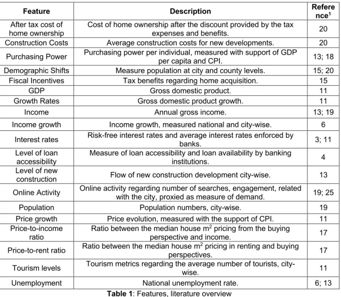
Feature Description Refere_nce1

After tax cost of

home ownership Cost of home ownership after the discount provided by the tax expenses and benefits. 20 Construction Costs Average construction costs for new developments. 20

Purchasing Power Purchasing power per individual, measured with support of GDP _{per capita and CPI.} 13; 18 Demographic Shifts Measure population at city and county levels. 15; 20

Fiscal Incentives Tax benefits regarding home acquisition. 15 GDP Gross domestic product. 11 Growth Rates Gross domestic product growth. 11

Income Annual gross income. 13; 19 Income growth Income growth, measured national and city-wise. 6

Interest rates Risk-free interest rates and average interest rates enforced by _banks. 3; 11 Level of loan

accessibility

Measure of loan accessibility and loan availability by banking

institutions. 4 Level of new

construction Flow of new construction development city-wise. 13 Online Activity Online activity regarding number of searches, engagement, related _{with the city, proxied as measure of demand.} 19; 25

Population Population numbers, city-wise. 19 Price growth Price evolution, measured with the support of CPI. 11 Price-to-income

ratio Ratio between the median house m

2 _{pricing from the buying}

perspective and income. 17 Price-to-rent ratio Ratio between the median house m_{perspectives.} 2 pricing in renting and buying 17 Tourism levels Tourism metrics regarding the average number of tourists, city-_wise. 11 Unemployment National unemployment rate. 6; 13

Table 1: Features, literature overview

Every feature used by past researchers is connected to some extent to the economic situation of each country, city, and its behaviors when exposed to external shocks, the end-goal being to evaluate how the reaction to this shock impacts the housing market. Present in the table above, is a summary overview of the most relevant features mentioned in the literature review.

3. METHODOLOGY

As an overview, from all the features gathered during the literature review, present in the table below, is a summary of which will be used in this research’s analysis.

Feature Proxy (if required) Used during _research

After tax cost of home ownership

Monthly mortgage price, included the annual tax

related to income owning. Yes

Construction Costs - No

Purchasing power Consumer price index. Yes

Demographic Shifts - No

Fiscal Incentives - No

GDP - Yes

Growth Rates GDP, GDP per capita and unemployment. Yes

Income - Yes

Income growth GDP per capita growth. Yes Interest rates Average implicit interest rates charged by banks _{during mortgage operations.} Yes

Level of loan

accessibility Interest rate growth, number of transactions in the housing market. Yes Level of new

construction - No

Online Activity Google search index, AirBnB and HomeAway _{metrics provided by AirDNA.} Yes

Population - No

Price growth - No

Price-to-income ratio - No

Price-to-rent ratio Monthly mortgage price against monthly rent price. Yes Tourism levels Number of sleepover operators in Lisbon, short-term _{rental permit requests} Yes

Unemployment - Yes

Table 2: Features, methodology overview

The process of analyzing Lisbon’s housing market will be based around concepts discussed in the literature review, it is important to take into consideration that most of the methods mentioned in the literature review cannot be directly re-performed with Portuguese data since its availability it is not the same as in the United States, however, the concepts behind the frameworks and metrics utilized will be kept and used as core of the analysis.

The first step was fetching all the necessary data with the biggest timeframe possible to make sure there is enough historical background available to compare

different economic situations. Data was obtained via INE (National Statistics Institute) and PORDATA, a Portuguese database repository, Google Trends, Turismo de Portugal and World Bank. From the literature review the most important KPIs to support the current housing prices are among, but not limited to interest rates, income, economic indicators (e.g. GDP, unemployment), construction costs, tourism levels and city population.

Data utilized in the research is limited to Lisbon district, and only considering construction utilized in familiar housing, e.g. office buildings and commercial buildings’ evaluation are not present or considered to any of the values shown.

Regarding the feature space to be utilized in the analysis, it is important to note that it is not limited to the features presented in the literature review, as an area of impact on the housing market, (e.g. tourism), can be developed in several different indicators which will help us with the support, or not, speculation effects.

It is fundamental for the analysis that the timeframe is able to capture free speculation scenarios (e.g. no speculative bubble present), as well as the opposite, so that the feature evolution that led up to that bubble, and subsequent burst, can be analyzed.

The ideal timeframe for all the analysis made on the features would be a full monthly-year space, but when this is not possible, a monthly cluster scenario (e.g. quarterly, semesterly) will be taken into consideration.

When referring to currency amounts, it is important to minimize the impact inherent time deviations (e.g. inflation), from past observations in order to be accurately compared against more recent ones. To perform this, two approaches were considered, for domestic currency, euro (€), inflation up until 2018 was imputed onto

the values, inflation was calculated with the support of the Portuguese CPI and subsequent computation of the YoY differences. For non-domestic currencies, a conversion to euro (€) was performed, using the currency pair from the referenced original date, and then, similarly to the approach used previously, inflation was again imputed in the values. By performing these calculations, the error obtained from any possible monetary value comparisons will be kept to a minimum, as the time deviation present in the data was normalized.

3.1. R

C

From the literature review, we concluded that, despite not being limited to, there were two ratios which were considered as highly relevant in analyzing the current housing market.

In both, price-to-income ratio and price-to-rent ratio, the goal is to analyze the magnitude of the difference between median housing prices and median income values, and the same for median housing prices and median rent values. As this research is only considering Lisbon as location. This provides a great overview regarding the housing market when compared with other local indicators, in this case, the income and the rent prices, which most of the time are correlated with the housing prices, but in an equilibrium situation, there should not be a major difference between a monthly payment of a house, and monthly rent.

By analyzing these ratios it will be possible to have a better understanding regarding the current economic situation of the city, (e.g. if the price-to-income ratio keeps increasing rapidly, it indicates that the house prices are growing faster than the actual incomes, supporting the idea of a possible bubble.).

As a limitation, accurate and up to date income information is not made publicly available, despite the minimum national wages, there is not a drilldown available and no historical information besides occasional reports done by public domain institutions.

The approach used to mitigate this lack of data was to deconstruct both ratios in their actual concept, the difference between house buying, rental and income values, it is relevant to keep the concept mentioned by (Himmelberg et al., 2005) when describing the imputed-rent framework which emphasized the actual cost of owning a house, not being limited to simply the monthly mortgage payments, but also including other factors such as, alternative investment opportunities, so that when comparisons are made between rental and buying costs, the researcher can analyze the most information possible so it can develop a more accurate and precise finding.

3.2. E

For the question at hand in this research, exploratory data analysis (EDA), is the most suitable approach as there is not a highly precise technique which could answer it leaving no room for future work.

EDA is a set of techniques from data analysis field which leaves space for alternative possibilities, it does not give a binary scenario result, but instead supports the investigator in choosing a direction when conducting its research, EDA ends up being a systematic way to investigate relevant information from different perspectives, instead of insisting in one set of data and re-analyzing it until it proves the researcher’s question without leaving space for further understanding (Yu, 1977).

As the research question2 _{is non-probabilistic, the focal point should be all the} available data at hand and, since EDA is not a standalone approach, how can the

researcher make use of different exploratory techniques available, to create new hypothesis which will support the initial question. Traditionally, EDA can be characterized by an emphasis on the substantive understanding of data that will attempt to address the research question, an emphasis on graphical representations, a focus on tentative model building and hypothesis generation and residual analysis (e.g. the difference between predicted and observed values), and, positions of flexibility regarding which methods to apply when analyzing data (Behrens, 1997).

For what concerns this research, graphical representations and understanding the underlying features which are directly connected to the core question will be the focal points of EDA.

The goal of EDA is to discover patterns and hidden relations in the data and evaluate if those can support the initial research question with either findings or the development of alternative hypothesis. It also supports the researcher in dealing with common data quality problems which might include but not limited to missing values or outliers, it ends up serving as basis for having the perfect foundations to build the research upon (Fedderke & Klitgaard, 1998).

From the techniques described in the literature review, most of them were suited to analyze the United States housing market and economy, unfortunately, due to limitations in data governance and data availability, it was not possible to match all the features used by previous researchers with the same correspondent features belonging to the Portuguese scenario.

Instead, this research kept the core concepts behind those techniques and applied those to proxy features, while trying to keep the differences between the basis of

previous studies’ insights to a minimum while also providing accurate insights for the Portuguese environment as well as opportunities for new hypothesis development.

3.3. A

Future growth in number of transactions was the feature selected to act as proxy for quantifying the demand in the housing market. Future growth is the future growth rate based on the present number of transactions, considering -_! as the number of transactions in the beginning of the period and ∆!%& as the future growth rate, the

number of transactions in ) + 1 should be equal to -!∗ ∆!%&. During the analysis, a

multilinear regression model was established in order to attempt to measure what features have the most impact on demand. The end goal being to evaluate the volatility of each independent features and understand how this relates with their impact on the target variable.

As all the independent features are not in the same scale, to achieve a better understanding of the final coefficients obtained, a min-max scaling3_{, was performed in} all the features present, so their values could be compromised between 0 and 1.

Volatility was proxied via the standard deviation of each feature (Baillie & DeGennaro, 1990; French, Schwert, & Stambaugh, 1987; Shiller, 1980). Standard deviation is often used as a measure of volatility in the stock market, to measure price and return volatility, during the research, the exact same approach was considered, to measure individual feature volatility of the independent features preset in the multilinear regression model.

3 _{Min-max scaling,} !!"#"!#

#"$%"#"!# , where x$ is the current feature observation, X%$& is the minimum value of the feature set and X is the maximum value of the feature set.

Model performance was evaluated via the adjusted R2_{, since it explains from 0 to} 100% the percentage of data variance explained by the model, and residual analysis, considering the difference between predicted and actual values, and evaluating their quantiles distribution against a quantile distribution from a t-Student distribution sample.

4. ANALYSIS AND RESULTS

4.1. E

In the literature review, previous researchers mentioned the importance of analyzing the surrounding economic scenario where the target housing market is inserted. A limitation of this part of the research is the lack of accurate sources with these indicators segmented by cities, instead were used the same indicators, but on a nationwide scale.

Figure 1: Portuguese GDP, EUR, source: World Bank

Figure 2: Portuguese GDP Growth, source: World Bank

100 000 € 120 000 € 140 000 € 160 000 € 180 000 € 200 000 € 220 000 € 240 000 € 2000 2001 2002 2003 2004 2005 2006 2007 2008 2009 2010 2011 2012 2013 2014 2015 2016 2017 2018 GD P ( Mi lli o n ) Year

Portuguese GDP

Portuguese GDP Growth

Statistics Portuguese GDP, Million Portuguese GDP Growth Min €100,318.54 -4.32% 1st Quantile €163,791.84 1.76% Median €183,389.80 3.68% 3rd Quantile €201,844.22 4.33% Max €222,072,95 5.68% Standard Deviation €36,069.55 2.84% Size 19 18

Table 3: Summary Statistics, GDP and GDP Growth

Figures 1 and 2 exhibit the recent nationwide growth in terms of economic development, it is also worth to notice the recession period suffered around the global financial crisis of 2008, which served as starting point for the Portuguese financial crisis suffered between 2010 and 2014, which is clearly reflected in the Figure 2, as a period of increased volatility is present between 2008 and 2014. During the last three years growth has been stable, but it is also showing signs of a deceleration which suggest a new crisis might be erupting, the only time GDP has ever been this high was in 2008 and it rapidly dropped because of the global crisis which then lead into the 2010-2014 Portuguese crisis.

Figure 3: Portuguese GDP per-capita growth, source: World Bank Statistics GDP Per Capita Growth

Min -1.71% 1st Quantile 2.68% Median 3.42% 3rd Quantile 4.86% -2,00% -1,00% 0,00% 1,00% 2,00% 3,00% 4,00% 5,00% 6,00% 7,00% 2000 2001 2002 2003 2004 2005 2006 2007 2008 2009 2010 2011 2012 2013 2014 2015 2016 2017 2018 GD P P er C ap it a Gr o wt h Year

Max 6.63% Standard Deviation 2.34%

Size 18

Table 4: Statistics summary, Portuguese GDP per capita growth

During the 2008-2014 crisis, GDP Per Capita suffered as it was expected during a recession period, decreasing on a year basis. Since the end of the crisis, it has been increasing again, on average, 4.77% per year during the last three years, from the entire timeframe available, it is also worth to notice the high volatility present in the data. GDP per capita it is currently at the highest values ever recorded for Portugal, meaning there never was a timeframe with as much available to spend.

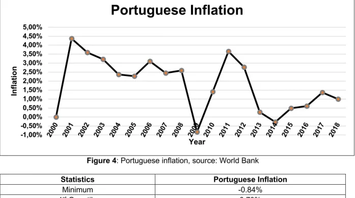
Figure 4: Portuguese inflation, source: World Bank

Statistics Portuguese Inflation

Minimum -0.84% 1st _{Quantile 0.70%} Median 2.32% 3rd _{Quantile 3.02%} Maximum 4.37% Standard Deviation 1.48% Size 18

Table 5: Statistics summary, inflation

Inflation, which is the YoY between CPI, has grew on average 1% per year from the last three years, when compared with GDP per capita, it makes the assumption of having a bigger purchasing power even more accurate, as citizens are having more available income and there is a surplus when comparing the differences between these

-1,00% -0,50% 0,00% 0,50% 1,00% 1,50% 2,00% 2,50% 3,00% 3,50% 4,00% 4,50% 5,00% 2000 2001 2002 2003 2004 2005 2006 2007 2008 2009 2010 2011 2012 2013 2014 2015 2016 2017 2018 In fla tio n Year

Portuguese Inflation

two indicators. Considering 2010 as basis, there is currently a +10% increase on the CPI, and when considering 2010 as basis for GDP per capita, there is currently a +26% increase in the same time frame, leaving people with surplus regarding purchasing power they had when compared directly with inflation.

Figure 5: Portuguese Unemployment Rate (%), source: World Bank Statistics Unemployment Rate

Minimum 3.81% 1st _{Quantile 6.59%} Median 7.96% 3rd _{Quantile 11.76%} Max 16.18% Standard Deviation 3.74% Size 19

Table 6: Statistics summary, Portuguese unemployment rate

Unemployment suffered with the Portuguese crisis of 2010-2014, which is expected as the economy’s health declines with it also declines the business incentive, and with it, job opportunities. On the last three years, unemployment rate has been declining on an average rate of -18% per year, again proving the current Portuguese economic prosperity. 0% 2% 4% 6% 8% 10% 12% 14% 16% 18% 2000 2001 2002 2003 2004 2005 2006 2007 2008 2009 2010 2011 2012 2013 2014 2015 2016 2017 2018 Un em p lo ym en t Ra te Year

4.2. P

,

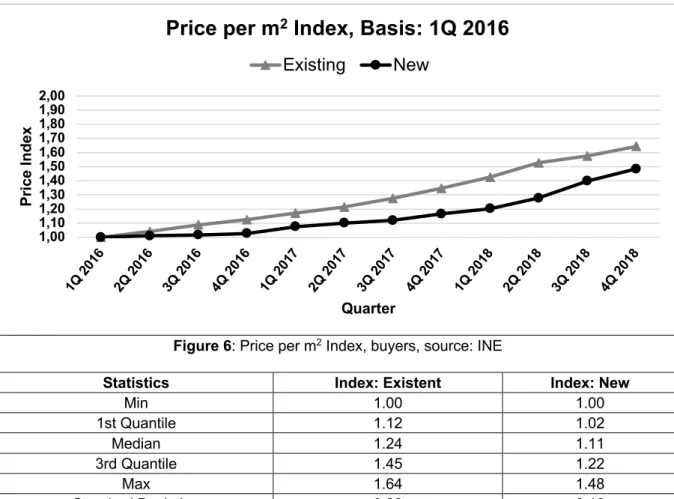
Figure 6: Price per m2 _{Index, buyers, source: INE}

Statistics Index: Existent Index: New

Min 1.00 1.00 1st Quantile 1.12 1.02 Median 1.24 1.11 3rd Quantile 1.45 1.22 Max 1.64 1.48 Standard Deviation 0.22 0.16 Size 12 12

Table 7: Summary statistics, price per m2 _index

Since 2016, the increase of housing prices in both new and existing construction has been steadily increasing. Between 2016 and 2018, a difference of 64% in existing construction and 48% on new construction was observed. Which means that in a 3-year timeframe, householders achieved a possible return on investment of 64% before considering expenses and taxes related to owning a house, and in cases which houses were bought with the sole purpose of increase in value, expenses beside taxes do not nearly exist. Such high increase in a relatively small timeframe, encourages buyers and common investors which might at the time not even considering real estate on their portfolios, to acquire real estate assets with the sole purpose of selling them later in time based on the belief that prices will keep increasing in the future.

1,00 1,10 1,20 1,30 1,40 1,50 1,60 1,70 1,80 1,90 2,00 1Q 2016 2Q 2016 3Q 2016 4Q 2016 1Q 2017 2Q 2017 3Q 2017 4Q 2017 1Q 2018 2Q 2018 3Q 2018 4Q 2018 Pr ic e In d ex Quarter

Price per m

_{Index, Basis: 1Q 2016}

A speculative scenario happens when there is an exaggeration of the beliefs behind these increases, considering only the scenario that, if it had increased in the previous 3-year period, it will be continuing to increase on the upcoming period with the same magnitude.

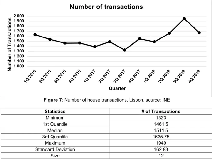
Figure 7: Number of house transactions, Lisbon, source: INE Statistics # of Transactions Minimum 1323 1st Quantile 1461.5 Median 1511.5 3rd Quantile 1635.75 Maximum 1949 Standard Deviation 162.93 Size 12

Table 8: Summary statistics, number of transactions

The number of transactions in the housing market verified between 2016 and 2018 is constant without too much variance reported. However, we can observe that the highest differences in transaction numbers happened at the same time of the highest increases in construction prices, Figure 8, (2018, 3rd _{and 4}th _{quarters), which, according} to the literature, continues to support the idea of investing due to simple beliefs of the asset having a higher value tomorrow.

1 000 1 100 1 200 1 300 1 400 1 500 1 600 1 700 1 800 1 900 2 000 1Q 2016 2Q 2016 3Q 2016 4Q 2016 1Q 2017 2Q 2017 3Q 2017 4Q 2017 1Q 2018 2Q 2018 3Q 2018 4Q 2018 Nu m b er o f T ra n sa ct io n s Quarter

Number of transactions

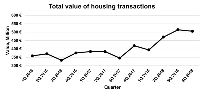
Figure 8: Total transaction value housing market, Lisbon, source: INE

Figure 9: Average transaction value for housing market, Lisbon, source: INE

Statistics Total Value, (Million €) Average Value Per Transaction (€)

Minimum €332.51 €219,962.55 1st _{Quantile €367.65 €253,122.75} Median €383.93 €262,397.05 3rd _{Quantile €431.56 €272,161.11} Maximum €514.06 €303,028.79 Standard Deviation €60.62 €23,088.32 Size 12 12

Table 9: Summary statistics, total and average value per transaction

From the observation of Figures 7, 8 and 9, a significant increase in housing price is noticed, when comparing both, beginning of 2016 and fall 2018, there is a slight difference between the number of transactions occurred (+2.3%), but the difference in

300 € 350 € 400 € 450 € 500 € 550 € 600 € 1Q 2016 2Q 2016 3Q 2016 4Q 2016 1Q 2017 2Q 2017 3Q 2017 4Q 2017 1Q 2018 2Q 2018 3Q 2018 4Q 2018 Va lu e, M ill io n Quarter

Total value of housing transactions

200 000 € 210 000 € 220 000 € 230 000 € 240 000 € 250 000 € 260 000 € 270 000 € 280 000 € 290 000 € 300 000 € 310 000 € 1Q 2016 2Q 2016 3Q 2016 4Q 2016 1Q 2017 2Q 2017 3Q 2017 4Q 2017 1Q 2018 2Q 2018 3Q 2018 4Q 2018 Av g Va lu e p er T ra n sa ct io n Quarter

value traded (+41%) is much higher, concluding that the average household price increased significantly despite the market demand staying stable, and that this new price increasing did not drove away investors from the housing market, and instead brought more money into it, despite being in an all-time high value scenario. The only belief behind investors in all time high scenarios is the idea that the current valuation is not fair, despite being the highest of all time, and that in the future, this value will eventually increase further.

County Price per m

2 _(€) YoY 2S 2017 1S 2018 2S 2018 Ajuda 8.77 10 10.83 23.49% Alcântara 8.87 9.66 10.49 18.26% Alvalade 9.67 10.37 11.34 17.27% Areeiro 9.70 10.44 10.87 12.06% Arroios 9.05 9.76 10.60 17.13% Avenidas Novas 10.15 10.96 12.54 23.55% Beato 9.23 9.57 10.11 9.53% Belém 10 10.77 11.58 15.80% Benfica 8.81 9.26 10.20 15.78% Campo de Ourique 10.94 11.35 12.18 11.33% Campolide 9.93 11.56 12.43 25.18% Carnide 10.91 10.96 12.31 12.83% Estrela 10.11 11.82 12.80 26.61% Lumiar 9.46 9.61 10.42 10.15% Marvila 8.42 9 9 6.89% Misericórdia 11.64 12.33 13.38 14.95% Olivais 8.64 9.29 10.07 16.55%

Parque das Nações 11.70 12.28 13.12 12.14%

Penha de França 8.71 9.57 10.18 16.88%

Santa Clara 6.82 7.65 8.31 21.85%

Santa Maria Maior 9.78 11.70 11.93 21.98%

São Domingos de Benfica 10.07 10.79 11.39 13.11%

São Vicente 10.03 10.92 12.07 20.34%

Table 10: Rental prices per county, source: INE

Statistics 2S 2017 1S 2018 2S 2018 Minimum €6.82 €7.65 €8.31 1st Quantile €8.86 €9.60 €10.37 Median €9.74 €10.61 €11.37 3rd Quantile €10.12 €11.40 €12.34 Maximum €11.70 €13.10 €14.10 Standard Deviation €1.11 €1.26 €1.40 Size 24 24 24

Table 11: Statistics summary, rental prices per county

Rental prices increased on average 17% between fall 2017 and fall 2018, meaning a regular 3-person family household around 90m2 _{would cost approximately something} between 750€ and 1269€. This increase in rental prices drove people away from renting into buying, but in this case, it is important to notice the difference between buyers as investors, and buyers who are effectively living in the household they just bought, since one is contributing to the speculative scenario with the belief the asset will increase in the future, and the other is only weighting an opportunity to save money when comparing monthly cost of rentals against monthly cost of owning a house.

County New Rental Agreements YoY (%) 2S 2017 1S 2018 2S 2018 Ajuda 240 221 201 -16.25% Alcântara 293 278 282 -3.75% Alvalade 429 413 417 -2.80% Areeiro 259 227 257 -0.77% Arroios 612 607 619 1.14% Avenidas Novas 406 360 372 -8.37% Beato 175 181 169 -3.43% Belém 187 173 161 -13.90% Benfica 388 362 368 -5.15% Campo de Ourique 370 343 327 -11.62%

Campolide 193 167 176 -8.81% Carnide 88 91 102 15.91% Estrela 350 311 341 -2.57% Lumiar 435 421 429 -1.38% Marvila 68 81 65 -4.41% Misericórdia 262 207 214 -18.32% Olivais 152 173 152 0.00%

Parque das Nações 286 267 265 -7.34%

Penha de França 442 452 468 5.88%

Santa Clara 176 166 145 -17.61%

Santa Maria Maior 181 163 158 -12.71%

Santo António 218 214 208 -4.59%

São Domingos de Benfica 470 477 460 -2.13%

São Vicente 300 295 287 -4.33%

Table 12: Number of new rental agreements in Lisbon, source: INE

Statistics 2S 2017 1S 2018 2S 2018 Minimum 68.00 81.00 65.00 1st _{Quantile 185.50 173.00 167.00} Median 274.00 247.00 261.00 3rd _{Quantile 392.50 360.50 369.00} Maximum 612.00 607.00 619.00 Standard Deviation 133.41 130.98 136.22 Size 24 24 24

Table 13: Statistics summary, number of new rental agreements

The decrease in rental agreements justifies the cost difference between actually owning and renting a house, on average, there was a -5% decrease in rental agreements in Lisbon.

All data related to the current buying and renting market leads to the conclusion that as time goes by and prices increase in both markets, despite a faster increase in the buying market, people are moving from the rental to buying, most likely because of cost related reasons.

There is a limitation when considering the ability to study the cost impact on the exchanges between rental and buying prices, since the data regarding wages in Lisbon is misleading, as the official average wage estimate is at around 860€ gross per month, but the actual values, according Social Security estimates, are around 1,294€ gross monthly, in both cases, considering a 14-month yearly period. As these are averaged values, there is a high possibility of outliers influencing this metric, as the minimum national wage is set at 600€ monthly gross, an increase of +3.4% when compared to last year, which makes any sort of conclusion with an assumption related with wages to be inaccurate or not as precise.

This enabled the research to follow other perspective, the source of actual funds being invested in Lisbon, as well as the average cost benefit of buying when compared to renting.

4.3. C

,

,

House mortgages are subject to a down payment on the house (between 10% and 20% of the house after a bank evaluation), and subsequent monthly payments with interest attached for the amount of the mortgage.

These interest rates are subject to two main components, one established by each bank, the spread and other one established by the Central European Bank, the EURIBOR, which can be a 3-month rate or a 6-month rate, on top of these two rates, banks also add markups for profit, but in the end, these represent much less percentage of the total interest rate than the two mentioned previously.

Year Euribor Periods, Rates in (%)

3m 6m 9m 12m