A 2D Hopfield Neural Network approach to mechanical beam damage detection

Noname manuscript No. (will be inserted by the editor)

A 2D Hopfield Neural Network approach to

mechanical beam damage detection

Juliana Almeida · Hugo Alonso · Pedro Ribeiro · Paula Rocha

Received: date / Accepted: date

Abstract The aim of this paper is to present a method based on a 2D Hop-field Neural Network for online damage detection in beams subjected to external forces. The underlying idea of the method is that a significant change in the beam model parameters can be taken as a sign of damage occurrence in the structural system. In this way, damage detection can be associated to an identification prob-lem. More concretely, a 2D Hopfield Neural Network uses information about the way the beam vibrates and the external forces that are applied to it to obtain time-evolving estimates of the beam parameters at the di↵erent beam points. The neural network organizes its input information based on the Euler-Bernoulli model for beam vibrations. Its performance is tested with vibration data generated by means of a di↵erent model, namely Timonshenko’s, in order to produce more re-alistic simulation conditions.

Keywords 2D Hopfield Neural Network · Euler-Bernoulli beam model · Timoshenko beam model· Damage detection

J. Almeida· P. Rocha

Faculdade de Engenharia da Universidade do Porto, Rua Dr. Roberto Frias, 4200-465 Porto, Center for Research & Development in Mathematics and Applications (CIDMA) - Universi-dade de Aveiro, Portugal

E-mail: almeidajfc@gmail.com; mprocha@fe.up.pt H. Alonso

Universidade Lus´ofona do Porto, Rua Augusto Rosa, 4000-098 Porto, Universidade de Aveiro, 3810-193 Aveiro, Center for Research & Development in Mathematics and Applications (CIDMA) - Universidade de Aveiro, Portugal

E-mail: hugo.alonso@ua.pt P. Ribeiro

DEMec/IDMEC, Faculdade de Engenharia da Universidade do Porto, Rua Dr. Roberto Frias, 4200-465 Porto

E-mail: pmleal@fe.up.pt

Click here to download Manuscript: mssp_v14.pdf Click here to view linked References

1 2 3 4 5 6 7 8 9 10 11 12 13 14 15 16 17 18 19 20 21 22 23 24 25 26 27 28 29 30 31 32 33 34 35 36 37 38 39 40 41 42 43 44 45 46 47 48 49 50 51

MULTIDIMENSIONAL SYSTEMS AND SIGNAL

PROCESSING Vol. 26 Nº. 4 p. 1081-1095

1 Introduction

Structural health monitoring using vibration based methods has shown to be a feasible approach to detect and locate damage. For economical and safety reasons, detecting beam cracks in their growth at an early stage is an important issue. This topic has been discussed by several authors and di↵erent approaches were proposed.

Some of the contributions use the fundamental mode shape as the most typical dynamic property for damage localization and quantification [1]. In beams with fatigue cracks, the control of the excitation force level is used for damage detection and does not require a comparative measurement on an intact structure [2]. In [3], the authors study the detection of fatigue damage on a beam using experimentally obtained modal parameters. The use of the modal parameters is justified since any beam can be considered as a dynamic system characterized by sti↵ness, mass and damping coefficients. When a beam su↵ers damage, the frequency response func-tions will change and the modal parameters of the system will also change [4]. This change can be taken as an early sign of damage occurrence in the structural system. In this way, damage detection can be associated to a problem of tracking parameter variations through appropriate estimation techniques, like the recursive least-squares and the Kalman filter [5]. Recently, a Hopfield Neural Network has been proposed in [6] for parameter estimation in one-dimensional dynamical pro-cesses. That network detects well parameter changes and can therefore be applied to damage detection. Here, in order to take into account the higher dimensionality of the process, a 2D version of that network is proposed. The 2D network enables a recursive update of the parameter estimate both in time and (one-dimensional) space. The estimate at a certain time instant and beam point depends on the esti-mate, vibration data and external forces information at previous time instants and neighbouring beam points. The way how the network organizes the data collected from the beam is based on the Euler-Bernoulli model for beam vibration. This model was chosen due to its simplicity.

The proposed identification method is illustrated by means of simulations. In order to produce a more realistic simulation environment, the proposed damage detection procedure is tested using data simulated from a di↵erent, more complex model, namely a Tiomoshenko beam to which a damage is inflicted at a certain time instant. These data are obtained using a p-finite element, with appropriate displacement shape functions, of a beam model based on Timoshenko’s theory for bending. The crack is represented by a small indentation on the beam, with consequent changes in its mass and sti↵ness.

The remainder of the paper is organized as follows. Section 2 presents the parameter estimation method for beam damage detection proposed here. This is followed by a reformulation of the damped Euler-Bernoulli beam model that allows for a better use of our methods described in Section 3. Section 4 explains how the simulated data were obtained and presents the corresponding damage detection results. The conclusions are drawn in Section 5.

1 2 3 4 5 6 7 8 9 10 11 12 13 14 15 16 17 18 19 20 21 22 23 24 25 26 27 28 29 30 31 32 33 34 35 36 37 38 39 40 41 42 43 44 45 46 47 48 49 50 51

2 Parameter identification via 2D Hopfield neural networks

The use of Hopfield Neural Networks (HNN) has proved to be an efficient method for online parameter estimation in one-dimensional processes [6]. Such networks are basically nonlinear dynamical systems with an adequate structure, whose out-puts are the time-evolving estimates of the relevant parameters. In [6], a special architecture was proposed that guarantees that the parameter estimates converge to their real values under some mild theoretical assumptions. Motivated by these results, here a 2D HNN approach based on an extension of the 1D HNN introduced in [6] is proposed in order to deal with higher dimensional or distributed processes. Before describing its two-dimensional version, first the 1D HNN introduced in [6] is presented. This network is designed for one-dimensional dynamical processes with a linear parameter dependency, i.e., for which the dynamical equations can be rewritten as

y(t) = A(t) ✓, (1)

where ✓ denotes the vector of parameters to be estimated and the vector y(t) and the matrix A(t) can be computed from the process data and depend on the model structure. Note that, the process dynamics may be nonlinear; linearity is only a requirement for the parameter dependency. The HNN dynamics is then given by

˙ˆ✓(t) = 1 D ⇣_✓(t)ˆ ⌘_AT_(t)⇣_{y(t) A(t)ˆ✓(t)}⌘_{, (2)} where ˆ✓(t) represents the parameter estimate at time t, ˙ˆ✓(t) is the first time deriva-tive, D ⇣✓(t)ˆ ⌘ is a positive definite (and thus invertible) matrix defined as

D ⇣✓(t)ˆ ⌘= diag⇣ 2 ✓ˆ2i(t) ⌘

(3) and and are design parameters, chosen such that ✓i2 ] , [ and chosen to guarantee a suitable network performance (speed of convergence, robustness to noise in the data, etc.). Letting (t) = ✓ ✓(t) represent the estimation error,ˆ equation (2) can be equivalently written as

˙ (t) = 1 D (✓ (t)) A(t)TA(t) (t). (4) As shown in [6], the estimate trajectory ˆ✓(t) converges to the real parameter vector ✓ under mild theoretical conditions, as stated in the following theorem. Theorem 1 The equilibirium ⇤= 0 of the estimation error dynamics (4) is glob-ally uniformly asymptoticglob-ally stable if for all nondegenerate interval I⇢ [t0, +1[,

\ t2I

ker (A(t)) = 0. (5)

Note that, since A(t) depends on system data, this theorem presents a sort of persistent excitation condition, under which the neural network is able to estimate the model parameters.

Discretizing the HNN (2) using finite di↵erences for a discretization step of t, yields: 1 2 3 4 5 6 7 8 9 10 11 12 13 14 15 16 17 18 19 20 21 22 23 24 25 26 27 28 29 30 31 32 33 34 35 36 37 38 39 40 41 42 43 44 45 46 47 48 49 50 51

ˆ

✓(k) = ˆ✓(k) + 1 D ⇣✓(k)ˆ ⌘ AT(k)⇣y(k) A(k)ˆ✓(k)⌘, (6) where, for the sake of simplicity notation, ˆ✓(k), A(k) and y(k) now respectively stand for ˆ✓(k t), A(k t) and y(k t), k = 0, 1, . . ., the design parameter rep-resents _t and is the time shift operator, defined by ✓(k) = ˆˆ ✓(k + 1).

It can be shown that for t small enough the discrete 1D HNN (6) maintains the convergence properties of (2). Therefore, we shall take this as a basis for defining a discrete 2D HNN to be used in the sequel for parameter identification and damage detection in parameterized 2D processes defined over time and (one-dimensional) space.

Hence, consider a parameterized 2D process in the time/linear-space. Like in the 1D case, the parameter dependence is assumed to be linear and the system dynamics can be rewritten as

y(x, t) = A(x, t) ✓, (7)

where the vector y(x, t) and the matrix A(x, t) depend on the system signals and their partial derivatives and ✓ is a vector of fixed parameters.

In order to estimate the parameters ✓ along time and space, the following 2D version of the discrete 1D HNN (6) is proposed:

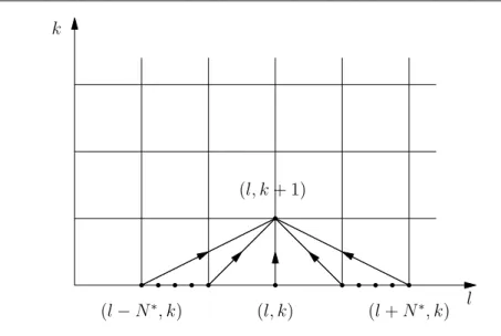
2✓(l, k) = ˆˆ ✓(l, k) + N⇤ X j= N⇤ ↵j(l) 1jF ⇣ ˆ ✓(l, k), A(l, k), y(l, k)⌘, (8) where l is the space discrete variable, k is the time discrete variable, 2 stands for the time-shift, i.e., 2h(l, k) = h(l, k + 1), 1 is the space-shift, defined by

j

1h(l, k) = h(l + j, k), the weights ↵j(l) are design coefficients,

F⇣✓(l, k), A(l, k), y(l, k)ˆ ⌘= 1 D (ˆ✓(l, k))AT(l, k)⇣y(l, k) A(l, k)ˆ✓(l, k)⌘, (9)

D (ˆ✓(l, k)) = diag⇣ 2 ✓ˆi 2

(l, k)⌘,

and and are suitable design parameters like in the 1D HNN. Moreover, again to keep notation simple, A(l, k) and y(l, k) are defined as the discretizations of A(x, t) and y(x, t), respectively, with spatial lag x and time lag t; more concretely,

A(l, k) = A(l x, k t) (10)

y(l, k) = y(l x, k t) (11)

for l = 0, 1, . . . and k = 0, 1, . . .

The updating structure of the nonlinear 2D di↵erence equation (8) is shown in Fig. 1.

In this setting, convergence to the parameter vector ✓ is understood as lim

k!1supl2Z ˆ

✓(l, k) ✓ = 0 . (12)

A theoretical analysis of this convergence problem will be presented elsewhere. In this paper, devoted to an application, we shall focus on the use of the proposed discrete 2D HNN for damage detection in vibrating beams.

1 2 3 4 5 6 7 8 9 10 11 12 13 14 15 16 17 18 19 20 21 22 23 24 25 26 27 28 29 30 31 32 33 34 35 36 37 38 39 40 41 42 43 44 45 46 47 48 49 50 51

l

k

(l, k + 1)

(l

N

_{, k)}

_{(l, k)}

_{(l + N}

_{, k)}

Fig. 1 Updating structure for Equation (8).

3 BEAM DAMAGE DETECTION

As mentioned before, our approach consists in detecting damage on a beam by monitoring the online estimates of the parameters of a corresponding mathematical model. This is based on the idea that damage corresponds to a change on the beam characteristics, which is in turn translated into a change in the parameters of the model that describes the beam dynamics.

Note that the damage detection problem is treated in a 2D framework in spite of the beam length being finite. This type of approach is also frequent in repetitive processes, in the sense that it is also common to see a system that is finite in one of the directions to be treated as a 2D system (see [19], for instance). Looking at the damage detection problem in a 2D context allows us to choose di↵erent discretization steps in both directions, time and one-dimensional space, which is an advantage. Moreover, the smaller the step in one direction, the greater the number of points in that direction, and hence, in a certain sense, the greater the extension of that direction.

3.1 Beam model

Here, the beam is considered to be described by a damped Euler-Bernoulli model [8], i.e.,

µ ¨w(x, t) + c ˙w(x, t) + EI @ 4_w

@x4(x, t) = q(x, t), (13) where w(x, t) is the transversal displacement at instant t and location x, ˙w(x, t) and ¨w(x, t) are, respectively, the first and second derivatives of w(x, t) with respect to t, and the parameters µ, c, EI correspond to the mass, damping coefficient and sti↵ness, respectively. The external force q(x, t) is considered to be a harmonic

1 2 3 4 5 6 7 8 9 10 11 12 13 14 15 16 17 18 19 20 21 22 23 24 25 26 27 28 29 30 31 32 33 34 35 36 37 38 39 40 41 42 43 44 45 46 47 48 49 50 51

excitation with amplitude F and frequency ! applied at the middle point of the beam, i.e., q(x, t) = ✓ x L 2 ◆ F sin(!t) (14)

where L is the length of the beam and is the unit spatial impulse. Moreover, it is assumed that the beam is clamped at both ends, which corresponds to the following boundary conditions:

w(x, t)_|x=0,L= 0 and @w

@x(x, t)_x=0,L = 0. (15) Note that this model is linear in the parameters in the sense that it can be rewritten as

y(x, t) = A(x, t) ✓ (16)

with y(x, t) = ¨w(x, t), A(x, t) =h w(x, t)˙ @4_w

@x4(x, t) q(x, t) i and ✓ = [✓1 ✓2 ✓3]T = h c µ EI µ 1 µ iT , for instance.

The presence of the fourth spatial derivative of the deflection w(x, t), @_@x4w4(x, t), may cause computational problems. An alternative to overcome this drawback is to reformulate the original Euler-Bernoulli model. For this purpose, a procedure based on Galerkin’s method is used [9]. First, the transversal displacement w(x, t) is expanded in an orthonormal basis for the spatial component with time-dependent coefficients. This allows to obtain the natural vibrations forms for the beam as solutions of ODEs. These spatial functions can in turn be used to obtain the fourth spatial derivative @4_w

@x4(x, t).

More concretely, the deflection w(x, t) is written as

w(x, t) = 1 X i=1 gi(x) fi(t) , (17) and approximated as w(x, t) = M X i=1 gi(x) fi(t) , (18)

for some M , where the functions gi(x) correspond to natural vibration forms for a beam with clamped ends [10], i.e., each gi(x) is the solution of

d4g dx4(x) ⇣ 4 i g(x) = 0 g(0) = g(L) = 0 (19) dg dx(0) = dg dx(L) = 0, where each ⇣i is a solution of the equation

cos(⇣ L)cosh(⇣ L) = 1 . (20) 1 2 3 4 5 6 7 8 9 10 11 12 13 14 15 16 17 18 19 20 21 22 23 24 25 26 27 28 29 30 31 32 33 34 35 36 37 38 39 40 41 42 43 44 45 46 47 48 49 50 51

The values of ⇣i i = 1, 2, . . ., can be found in a table (see for instance pp. 371 of [11]).

Thus, gi(x) is given by

gi(x) = cosh(⇣ix) cos(⇣ix) ↵i(sinh(⇣ix) sin(⇣ix)) , (21) with

↵i= 1

sinh(⇣iL)sin(⇣iL)

. (22)

Here, for the sake of simplicity in the exposition, it is assumed that the value of M in (18) is taken to be 1, M = 1, i.e., only the first natural vibration mode is considered, and in this way the beam deflection is assumed to be given by

w(x, t) = g(x) f (t), (23)

where g(x) = g1(x) is given by (21) for ⇣1= 9.46 (see [11, Table D.3]).

Substituting (23) in (13) and recalling that q(x, t) = x L₂ F sin(!t), the Euler-Bernoulli equation, with the considered boundary conditions, is equivalent to: g(x) ¨f (t) + ✓1g(x) ˙f (t) + ✓2 d 4_g d x4(x)f (t) = ✓3 ✓ x L 2 ◆ F sin(!t). (24) Multiplying both sides of equation (24) by the function g(x), integrating with respect to x in the interval [0, L] and taking into account that w(x, t) = g(x)f (t), the following alternative formulation is obtained:

¨

w(x, t) + ✓1w(x, t) + ✓˙ 2⌘w(x, t) = ✓3K g(x) F sin(!t), (25) where K = g(L/2)_G with G =R₀Lg2_{(x) dx and ⌘ = ⇣}

14. This finally yields the equation

¨ w(x, t) | {z } y(x,t) = [ w(x, t)˙ ⌘w(x, t) K g(x) F sin(!t)] | {z } A(x,t) 2 4✓✓12 ✓3 3 5 | {z } ✓ . (26)

For a time discretization lag t and a spatial discretization lag x = _{m 1}L , corresponding to the division of the interval [0, L] into m 1 intervals of equal length, one obtains:

y(l, k) = A(l, k) ✓ (27)

where, following the previously introduced notation,

y(l, k) = y(l x, k t) and (28)

A(l, k) = A(l x, k t). (29)

Finally, it is not difficult to check that y(l, k) and A(l, k) can be obtained as

y(l, k) = ¨w(l x, k t) (30) A(l, k) = [ w(l x, k t)˙ ⌘ w(l x, k t) K g(l x) F sin(! k t)] (31) 1 2 3 4 5 6 7 8 9 10 11 12 13 14 15 16 17 18 19 20 21 22 23 24 25 26 27 28 29 30 31 32 33 34 35 36 37 38 39 40 41 42 43 44 45 46 47 48 49 50 51

4 Simulations

This section starts by presenting the Timoshenko model used to simulate vibration data di↵erent from those generated by the Euler-Bernouli model, on which the discrete 2D Hopfield Neural Network damage detection method is based. Then, the results of the application of this method to that data are presented.

4.1 Simulation model

In order to test the damage detection procedure, a di↵erent model, independent from the one employed in the damage detection algorithm, was used to gener-ate vibration data corresponding to healthy and damaged beams. Although being still within a simulation framework, this seems to be a more realistic situation, as it mimics the misfit between models and reality. The model used to simu-lated the beam vibration is based on a Timoshenko type p-version finite element and was introduced in [12] see also [13]). We used this model to obtain the data w(x, t), ˙w(x, t) and ¨w(x, t) from which y(x, t) and A(x, t) in (26) are constructed and then given as inputs in their discrete versions to the 2D HNN (8). For the sake of completeness, the main steps of the formulation are described here.

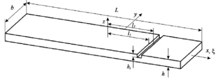
Although geometrical non-linearity was taken into account in [12], only the linear part of the model is now presented, because small displacements are con-sidered in the test cases of this paper. In this model, damage is represented by an always open notch or indentation, with corresponding mass and sti↵ness loss. The beam has rectangular cross section of thickness h and width b. Measured from the beams middle, the notch starts at x = l1and ends at x = l2, its depth is h1.

Fig. 2 Damaged beam with local and global coordinate system.

The displacement components along the beam axis, x, and in the direction perpendicular to it, z, are represented by u(x, z, t) and w(x, z, t), respectively. They are given by

u(x, z, t) = u0(x, t) + z ⇡0(x, t), w(x, z, t) = w0(x, t), (32) where superscript00000 represents the axis that crosses the undamaged cross section centroids, i.e. axis x, and t represents time; cross section rotations are represented by ⇡0_{(x, t).} 1 2 3 4 5 6 7 8 9 10 11 12 13 14 15 16 17 18 19 20 21 22 23 24 25 26 27 28 29 30 31 32 33 34 35 36 37 38 39 40 41 42 43 44 45 46 47 48 49 50 51

Note that the transversal displacement w(x, t) of the Euler-Bernoulli model corresponds to the w0(x, t) of the Timoshenko model. The derivatives ˙w(x, t) and

¨

w(x, t) are obtained by numerical di↵erentiation.

The longitudinal strain and the engineering shear strain are, respectively,

✏x(x, t) = @u 0 @x (x, t) + z @⇡0 @x(x, t) (33) xz(x, t) = @w 0 @x (x, t) + ⇡ 0 (x, t). (34)

The displacement components at axis x and the cross section rotation form vector d0( ¯⇠, t), which is expressed as the product of the hierarchical shape functions matrix N ( ¯⇠) by the vector of generalized displacements q(t):

d0( ¯⇠, t) = N ( ¯⇠)q(t) , 2 4u 0_{( ¯⇠, t)} w0_{( ¯⇠, t)} ⇡0_{( ¯⇠, t)} 3 5 = 2 4N u_{( ¯⇠)}T _{0 0} 0 Nw_{( ¯⇠)}T ₀ 0 0 N⇡_{( ¯⇠)}T 3 5 2 4qqwu(t)(t) q⇡(t) 3 5 , (35)

qu(t), qw(t) and q⇡(t) are vectors of generalized displacements. The matrix of shape functions N ( ¯⇠) is constituted by row vectors of longitudinal, transverse and rotation shape functions. To improve the accuracy of the discretization, the number of shape functions and generalized displacements in a finite element are increased. A non-dimensional co-ordinate, ¯⇠, was inserted in equation (35), as is common in finite elements; however, because one element is sufficient to describe the whole beam, the relation between ¯⇠ and x is simply ¯⇠ = 2x/L. The set of shape functions employed here is given in [12]; this set includes new functions which improve the efficiency of the p-version FEM in the presence of localized steep variations.

The material is assumed to behave in a linear elastic manner and to be isotropic, hence generalized Hooke’s law holds, so (without function arguments, in order to simplify the notation)

= D ✏ _,  x ⌧xz =  E 0 0 G  ✏x xz . (36)

In equation (36) E is the Young modulus and G is the shear modulus of elasticity, which is equal to _2(2+⌫)1 and ⌫ is the passion ratio and is the shear correction factor, which we assume to be 5+5⌫_6+5⌫ after [14]; and ✏ are vectors which contain, respectively, the non-zero stresses and the strains of interest here. The longitudinal strain can be written as

✏x = ⇥1 z⇤ 

✏p₀ ✏b0

, (37)

with ✏p₀ the longitudinal and z ✏b0 the bending strain.

Integrating along the normal stress, the shear stress and the moment the nor-mal stress about y, one obtains a longitudinal force per unit length, T , a transverse force per unit length, Q, and a moment per unit length, M . They are

1 2 3 4 5 6 7 8 9 10 11 12 13 14 15 16 17 18 19 20 21 22 23 24 25 26 27 28 29 30 31 32 33 34 35 36 37 38 39 40 41 42 43 44 45 46 47 48 49 50 51

 T M =  A B B D  ✏p₀ ✏b0 (38) Q = ( _Eh 2(1+⌫) xz, x 2 ⇥ _L 2, l1 ⇤ [⇥l2,L₂⇤ E(h h1) 2(1+⌫) xz, x 2 ]l1, l2[ , (39)

where A, B and D are the extension, coupling and bending coefficients, given by

A = ⇢ Eh , ⇥ L₂, l1⇤[⇥l2,L₂⇤ E(h h1) , ]l1, l2[ (40) B = ⇢ 0 , ⇥ L₂, l1⇤[⇥l2,L₂⇤ Eh1(h1 h) 2 , ]l1, l2[ (41) D = ( _Eh3 12 , ⇥ _L 2, l1 ⇤ [⇥l2,L₂⇤ E[h3_{+(h 2h} 1)3] 24 , ]l1, l2[ (42) The discontinuity in the cross section due to the localized change in the beam thickness a↵ects coefficients A, B and D. Actually, B would be zero in a rectan-gular, homogeneous beam, and only appears in this formulation because of the notch.

The equations of motion are obtained by applying the principle of virtual work, according to which

Win + WV + Wex= 0, (43)

where Win, WV and Wex are, respectively, the virtual work that the inertia, internal and external forces do under a virtual vector displacement d:

d = 2 4 wu ✓ 3 5 = N q. (44)

The virtual work of internal and inertia forces are respectively given by

WV = Z V ✏ dV (45) Win= Z V ⇢ dTd dV ,¨ (46)

where ¨d is the vector containing components of acceleration. More details on the above written virtual works can be found in [12]. The virtual work of the external forces is given in [15].

Without damping, the equation of motion in time domain are: 2 4M l _{0 0} 0 Mb ₀ 0 0 Mr 3 5 2 4q¨q¨wu(t)(t) ¨ q⇡(t) 3 5 + 2 4 0 0 Mlr 0 0 0 Mlr T_{0 0} 3 5 2 4qq¨¨wu(t)(t) ¨ q⇡(t) 3 5 + (47) + 2 4K0 K` 011 0 ` K 12 ` 0 K 21 ` K`b+ K`22 3 5 2 4qqwu(t)(t) q⇡(t) 3 5 + 2 4 0 0 Klr ` 0 0 0 Klr ` T 0 0 3 5 2 4qqwu(t)(t) q⇡(t) 3 5 = 2 4F E u(t) FE q (t) ME_(t) 3 5 , 1 2 3 4 5 6 7 8 9 10 11 12 13 14 15 16 17 18 19 20 21 22 23 24 25 26 27 28 29 30 31 32 33 34 35 36 37 38 39 40 41 42 43 44 45 46 47 48 49 50 51

⇥ FE

u (t), FwE(t), ME(t)⇤ T

is the vector of generalized external forces. Matrices M and K` are, respectively, the mass and sti↵ness matrices. Superscripts l, b, r and

indicate, respectively, longitudinal, bending, cross section rotation and shear e↵ects. Superscript lr represents longitudinal-rotation coupling that occurs due to damage and is reflected in the mass and linear sti↵ness matrix. The mass and sti↵ness matrices are given in [12], the vector of generalized external forces in [15]. Finally, introducing Rayleigh-type damping, with damping coefficients ↵ and , and writing the equations of motion in a more condensed form, yields,

(M + Mc_{)¨q(t) + ↵ (K}

` + K`c) ˙q(t) + (M + Mc) ˙q(t) + (K` + K`c) q(t) = F (t). (48)

Matrices Mcand K`crepresent couplings introduced by the notch.

4.2 Simulation results

In this section, the discrete 2D Hopfield Neural Network (8), with y, A and ✓ as defined in (26), is applied to detect damage in a beam. The vibration data in (26) were obtained using the Timoshenko model described in subsection 4.1 for a beam with the following characteristics (before the damage occurs): L = 0.5 m, E = 71.72⇥ 109_N/m2_{, I = 3.255⇥ 10} 8_m4_{, µ = 1.75 kg/m and c = 1808.7 N s/m}2_. Within this setting, the model initialising parameters are ✓1= _µc = 1033.5, ✓2 =

EI

µ = 1334.1 and ✓3= 1

µ = 0.5714. Then, damage was simulated at t = 0.1 s, and, as explained in Section 4.1 (second paragraph), was represented by an always open notch or indentation, with corresponding mass and sti↵ness loss, which translated into a change in all parameters ✓1, ✓2 and ✓3. The beam was subjected to a harmonic excitation with amplitude F = 1000 N and frequency ! = 3214.87 rad/s. The beam was spatially discretized in 27 equally spaced points xl= l x with l = 0, . . . , 26. Moreover, in equation (8), N⇤ was taken equal to 1 and the weights ↵j(l) were defined as in [18], i.e., at the beam ends we took

↵ 1(0) = 0 ↵0(0) = 26/27 ↵1(0) = 1/27 ↵ 1(26) = 1/27 ↵0(26) = 26/27 ↵1(26) = 0

in the middle of the beam

↵ 1(l) = 0.5/27 ↵0(l) = 26/27 l = 1, . . . , 25 ↵1(l) = 0.5/27 1 2 3 4 5 6 7 8 9 10 11 12 13 14 15 16 17 18 19 20 21 22 23 24 25 26 27 28 29 30 31 32 33 34 35 36 37 38 39 40 41 42 43 44 45 46 47 48 49 50 51

and finally

↵j(l) = 0 l < 0 or l > 26

taking into account that there is a finite number of discretization points in a beam of limited length. Note that, for each point l = 0, . . . , 26, the sum of the weights equals 1, and that more importance, corresponding to a weight of 26/27, is given to the data collected from that point, while less importance, corresponding to a distributed weight of 1/27, is given to the data collected from the neighbours of that point. Since in a realistic situation the real values of the parameters are not known, instead of considering the parameter estimation error, in order to analyze the performance of the damage identification method, we considered at each discrete time instant k 0 the error measure

ECH(k) = max

l ky(l, k) A(l, k)ˆ✓(l, k)k1 (49) and computed the average ECH(k) of the errors ECH(0), . . . , ECH(k). In the sequel, we examine the relative change in the average error from time k 1 to time k, given for k 1 by

er(k) =ECH(k) ECH(k 1)

ECH(k 1) ⇥ 100% . (50)

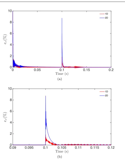
Figure 3 shows the results for the 2D HNN proposed here. It also shows, for com-parison purposes, the results of a 1D HNN approach based in the work presented in [6]. It can be seen that, when damage occurs at time t = 0.1 s, the relative change in the average error is greater for the 2D HNN. This means that our multi-dimensional approach presented here makes easier to detect damage. Furthermore, it presents more stable results, as the relative change in the average error does not oscillate after the initial identification phase, contrary to what happens with the 1D HNN approach.

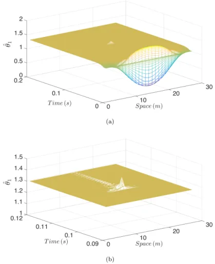
The 2D HNN proposed here can be used not only for damage detection but also for damage localization. Figure 4 depicts the time/space evolution of the ✓1 estimate produced by the network. It can be seen where damage occurs by observ-ing where the peak in the parameter estimate occurs after the initial identification phase.

Finally, note that the good results obtained by the 2D HNN were achieved in a context where the beam displacement data was generated by a model di↵erent from the one on which the network is based. Moreover, the velocity and acceleration data were contaminated with errors, since they were calculated using numerical di↵erentiation. For all this, the results suggest that the 2D HNN deals well with a model mismatch and is robust to noise in the data.

5 Conclusions

This paper presents a multidimensional neural network for mechanical beam dam-age detection. The network organizes the data collected from the beam based on the Euler-Bernoulli model for beam vibrations. In order to simulate a mismatch

1 2 3 4 5 6 7 8 9 10 11 12 13 14 15 16 17 18 19 20 21 22 23 24 25 26 27 28 29 30 31 32 33 34 35 36 37 38 39 40 41 42 43 44 45 46 47 48 49 50 51

Time (s) 0 0.05 0.1 0.15 0.2 er (% ) 0 2 4 6 8 10 1D 2D (a) Time (s) 0.09 0.095 0.1 0.105 0.11 0.115 0.12 er (% ) 0 2 4 6 8 10 1D 2D (b)

Fig. 3 (a) Time evolution of the relative change in the average identification error; (b) zoom around the time instant where damage occurs.

between this model and reality, we test the network using data from a di↵erent, more complex model, namely Timoshenko’s. The network deals well with the mis-match and is robust to noise in the data. It enables not only damage detection but also damage localization. The results are superior to those of a unidimensional neural network approach. For all this, we feel encouraged to incorporate the mul-tidimensional neural network method in an automatic system for online damage detection. Finally, we remark that this method can be extended to nD processes with n > 2 (where, as here, one of the variables is the time). This could, for instance, be useful for damage detection in vibrating plates.

1 2 3 4 5 6 7 8 9 10 11 12 13 14 15 16 17 18 19 20 21 22 23 24 25 26 27 28 29 30 31 32 33 34 35 36 37 38 39 40 41 42 43 44 45 46 47 48 49 50 51

(a)

(b)

Fig. 4 (a) Time/space evolution of a parameter estimate produced by the 2D HNN; (b) zoom around the time instant where damage occurs.

6 Ethical Statement

This work supported by FEDER founds through COMPETE–Operational Pro-gramme Factors of Competitiveness (”Programa Operacional Factores de Compet-itividade”) and by Portuguese founds through the Portuguese Foundation for Sci-ence and Technology (”FCT–Funda¸c˜ao para a Ciˆencia e a Tecnologia”), within the project PEst-C/MAT/UI4106/2011 associated with the Center for Research and Development in Mathematics and Applications (University of Aveiro) with COM-PETE reference FCOMP-01-0124-FEDER-022690, and the project INSTEAD, PTDC/EEA-AUT/108180/2008 with COMPETE reference

FCOMP–01–0124–FEDER–009842.

The authors hereby declare that there are no potential conflicts of interest in this work. 1 2 3 4 5 6 7 8 9 10 11 12 13 14 15 16 17 18 19 20 21 22 23 24 25 26 27 28 29 30 31 32 33 34 35 36 37 38 39 40 41 42 43 44 45 46 47 48 49 50 51

References

1. Maosen Cao, Lin Ye, Limin Zhou, Zhongqing Su, Runbo Bai, Sensitivity of fundamental mode shape and static deflection for damage identification in cantilever beams, Mechanical Systems and Signal Processing, 25, 630-643 (2011)

2. Do-Gyoon Kim, Soon-BokLee, Structural damage identification of a cantilever beam using excitation force level control, Mechanical Mechanical Systems and Signal Processing, 24, 1814-1830 (2010)

3. Maciej Radzi´nski, Marek Krawczuk, Magdalena Palacz, Improvement of damage detection methods based on experimental modal parameters, Mechanical Systems and Signal Process-ing, 25, 2169-2190 (2011)

4. Hanno Niemann, Joseph Morlier, Amir Shahdin, Yves Gourinat, Damage localization using experimental modal parameters and topology optimization, Mechanical Systems and Signal Processing, 24, 636-652 (2010)

5. Lennart Ljung, System identification (2nd ed): theory for the user, Prentice Hall PTR Upper Saddle River, NJ, USA (1999)

6. Hugo Alonso, Teresa Mendon¸ca, Paula Rocha, Hopfield neural networks for online param-eter estimation, Neural Networks, 22, 450-462 (2009)

7. Juliana Almeida, Hugo Alonso, Paula Rocha, A Neural network approach to damage detec-tion in Euler-Bernoulli beams subjected to external forces, 21st Mediterranean Conference on Control and Automation, Greece (2013)

8. O. A. Bauchau, J. I. Craig, Structural Analysis (Solid Mechanics and Its Applications), Springer Volume 163, pp. 173-221 (2009)

9. O. C. Zienkiewicz and K. Morgan, Finite Elements and Approximation, Wiley-Interscience, New York (1983)

10. W. Weaver, S. P. Timoshenko, D. H. Young, Vibration Problems in Engineering, John Wiley & Sons, New York (1990)

11. Alper Erturk, Daniel Inman, Piezoelectric Energy Harvesting, John Wiley & Sons (2011) 12. Vladimir Stojanovic, Pedro Ribeiro, Stanislav Stoykov, Non-linear vibration of Timo-shenko damaged beams by a new p-version finite element method, Computers and Structures, 120, 107-119 (2013)

13. Pedro Ribeiro, Vibration of Beams in the Elasto-Plastic and Geometrically Nonlinear Regime, Chapter 5, pp. 171-223, Lecture notes of CISM Advanced School Exploiting Non-linear Behaviour in Structural Dynamics. Editors D. Wagg and L. N. Virgin. Springer, Wien, New York, 2012.

14. T. Kaneko, On Timoshenko correction for shear in vibrating beams, Journal of Physics D 8, 19271936 (1975)

15. Pedro Ribeiro, A p-version, first order shear deformation, finite element for geometrically non-linear vibration of curved beams, International Journal for Numerical Methods in En-gineering, 61, 2696-2715 (2004)

16. Meyer, C. D., Matrix Analysis and Applied Linear Algebra, Philadelphia, PA: Society for Industrial and Applied Mathematics - SIAM (2000)

17. D. J. Schroeder, Astronomical optics (2nd edition). Academic Press (1999)

18. Almeida, J. Alonso, H., Rocha, P. A 2D neural network approach for beam damage detec-tion, 8th International Workshop on Multidimensional Systems (nDS13), Erlangen, Deutsch-land, September 2013.

19. Hladowski, L. and Galkowski, K. and Cai, Z. and Rogers, E. and Freeman, C.T. and Lewin, P.L. A 2D systems approach to iterative learning control for discrete linear processes with zero Markov parameters. International Journal of Control, 84(7), 1246-1262, 2011.

1 2 3 4 5 6 7 8 9 10 11 12 13 14 15 16 17 18 19 20 21 22 23 24 25 26 27 28 29 30 31 32 33 34 35 36 37 38 39 40 41 42 43 44 45 46 47 48 49 50 51