Transmission network expansion planning based on hybridization model of neural networks and harmony search algorithm

(1)

doi: 10.5267/j.ijiec.2011.08.018

Contents lists available at GrowingScience

International Journal of Industrial Engineering Computations

homepage: www.GrowingScience.com/ijiec

Transmission network expansion planning based on hybridization model of neural networks and harmony search algorithm

Mohammad Taghi Amelia , Mojtaba Shivaiea*, and Saeid Moslehpourb

a

Department of Electrical and Computer Engineering, Power and Water University of Technology (PWUT), Tehran, Iran

b_{Department of Electrical and Computer Engineering, University of Hartford, Hartford, USA}

A R T I C L E I N F O A B S T R A C T

Article history: Received 1 August 2011 Available online 10 August 2011

Transmission Network Expansion Planning (TNEP) is a basic part of power network planning that determines where, when and how many new transmission lines should be added to the network. So, the TNEP is an optimization problem in which the expansion purposes are optimized. Artificial Intelligence (AI) tools such as Genetic Algorithm (GA), Simulated Annealing (SA), Tabu Search (TS) and Artificial Neural Networks (ANNs) are methods used for solving the TNEP problem. Today, by using the hybridization models of AI tools, we can solve the TNEP problem for large-scale systems, which shows the effectiveness of utilizing such models. In this paper, a new approach to the hybridization model of Probabilistic Neural Networks (PNNs) and Harmony Search Algorithm (HSA) was used to solve the TNEP problem. Finally, by considering the uncertain role of the load based on a scenario technique, this proposed model was tested on the Garver’s 6-bus network.

Artificial intelligence Harmony search algorithm Probabilistic neural networks Transmission network expansion planning

1. Introduction

(2)

the factors affecting the system must be evaluated. One of these factors is transmission network losses. Reduction of these losses has been a priority for transmission network owners. In most cases, expansion costs and network losses are in conflict with each other, so the component losses in TNEP would be a multi-criteria decision making (MCDM) function. Accordingly, the network planner can construct the lines with lower losses and higher cost or construct the lines with lower costs but higher losses (Shayeghi et al., 2008; Youseef, 2001). Another factor affecting TNEP is uncertainty over Garver's famous offering of innovative ideas in 1970, at the same time as oil-crisis planners were being considered. Uncertainty refers to unknowns in the accurate diagnosis and determination of a case or a quantity. Uncertainties in power systems include the inability to determine the exact parameters of the system that are otherwise feasible. Irrespective of the uncertainty in the parameters, the process of transmission network expansion planning is a technical, economic optimization problem. But if this uncertainty were considered, the transmission network expansion problem would be more complicated. Some of these uncertainties include: (1) uncertainty in load, (2) uncertainty in fuel availability, (3) uncertainty in factor prices and financial parameters (Silva et al., 2005; Choi et al., 2005). Generally, the TNEP problem is a complicated optimization problem in which various methods are used. GA (Abdelaziz, 2000; Sadegheih & Drake, 2008), decimal codification genetic algorithm (DCGA) (Sadegheih & Drake, 2008) and TS have been used to solve the TNEP problem. Different hybridization models of AI were used (Al-Saba & El-Amin, 2002) such as the ANN with a Multi-Layer Perceptron (MLP) model, GA and TS. Therefore, in this paper, as a new approach, the hybridization model probabilistic neural networks (PNNs) and harmony search algorithm (HSA) were used to solve the TNEP problem. Accordingly, different solving states were considered as the neural network input and suitable alternatives with the features, which will be described in the next section, were considered as the neural network outputs. Therefore, the neural network is trained and the best solution set are made. Then, per every random input, the model used one of the best n-solution sets as an input for the HSA; network expansion was based on this. Also in this paper, DC load flow was used. Finally, by considering the uncertainty role in the load based on the scenario technique, this proposed model was tested on Garver’s 6-bus network.

2. Mathematical model (objective function) of the TNEP problem

As noted earlier, one of the expansion planning parameters which made optimal use of the transmission network losses was that its reduction is always a priority of network owners and the other one is uncertainties in load. On this basis, this study evaluated the role of losses in the network while considering these uncertainties, which was considered the objective function according to Eq. (1) (Shayeghi et al., 2008; Al-Saba & El-Amin, 2002). Also, Load Not Supply (LNS), in its normal state, is considered as a penalty factor in the objective function.

,

Objective Function :

( , ) 1

Y N

ij ij k b

i j k b B

TEC CL n ALC α r

∈Ω = ∈

= ∑ × +∑ + × ∑ (1)

where:

8760

Loss Loss

ALC =Loss C× ×K × (2)

2

( , )i j ij ij

Loss R I

∈Ω

= ∑ × (3)

where Ωis the set of all corridors, B the set of all buses, N_Y the expanded network adequacy (in years), TEC the total expansion cost of the network, CL_ijthe construction cost of each line in the

corridor i-j, ALC the annual losses cost of the network, Loss the total losses of the network, rbthe

load not supplied in bus b, αthe transfer coefficient of the load not supplied to the cost, R_ijthe

resistance of corridor i–j, I_ij the flow current of the corridor i–j, C_Lossthe cost of one kWh

(3)

The LNS component is the over load of the expanded network lines which hasn't arrived at the load center because of the power flow limitation and some of the load isn't supply. So, relating this component's cost to the consumed load value in the planning horizon, is affected by the considered scenario for the load growth. Of course, the value of LNS evaluation is very difficult to discern so in this study, it was considered as an approximate value for the coefficientα. Also, the constraints of the TNEP problem were set according from Eq. (4) to Eq. (9).

0

Sf + − =g d (4)

0

( )( ) 0

ij ij ij ij i j

f −γ n +n θ −θ = , ( , )∀ i j ∈ Ω (5)

0

( ij ij) ij

j

f n n f

i ≤ + , ( , )∀ i j ∈ Ω

(6)

, , ,

0≤nij ≤nij, n_i_j is integer variable, , ( , )∀ i j ∈ Ω (7)

0

( ) ,,

ij ij ij ij

Y = − y +n τ i ≠ j , ( , )∀ i j ∈ Ω (8)

0

0 ( ) ,,

ii i ij ij ij j i

Y y y n τ i j

∈

= + ∑ + ≠ , ( , )∀ i j ∈ Ω (9)

whereS is the branch-node incidence matrix,f the active power matrix in each corridor with elements f_ij ,g the generation vector, d the demand vector, θ the phase angle of each bus,γ_ijthe

total admittance of circuits in the corridor i-j, 0

ij

n the number of initial circuits in the corridor i-j, n_ij

the number of new circuits added to the corridor i-j, n_ijthe maximum number of constructible circuits

in the corridor i-j, f_ij the maximum transmittable active power through the corridor i-j, 0

ij

y the initial

admittance of the corridor i-j,τ_ijthe new circuit admittance of the corridor i-j,y_i₀the shunt

admittance at bus i, and Y the bus admittance matrix of the system.

Eq. (4) and Eq. (5) are DC load flow relationships and Eq. (6) points to the power-flow limitations. Eq. (7) requires transmission line expansion within the bounds of maximum line addition. Eq. (8) and Eq. (9) simply update the network admittance matrix with expansion (Eliassi et al., 2009).

3. Probabilistic neural networks

One of the most powerful neural networks is a Radial Basis Function (RBF). This network has more strategic benefits than perceptron neural networks (Christodoulou & Georgiopoulos, 2001). Probabilistic Neural Networks (PNNs) are a kind of radial-basis network suitable for classification problems. PNNs are feed forward networks which are built with three layers. The input layer, hidden layer and one output layer. In the hidden layer, an activation function is applied to the distance between the unknown input and the training example. PNNs estimate the probability density function for each class based on the training samples using similar probability density functions, which are calculated for each test vector.

(4)

4. Harmony search algorithm

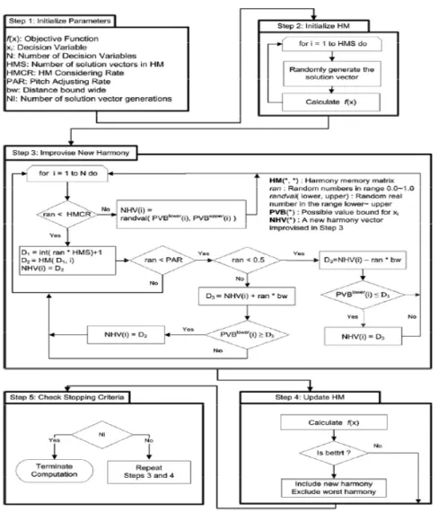
In researching TNEP, problems are solved using many algorithms (Sadegheih & Drake, 2008). The Harmony Search Algorithm (HSA) was recently developed in an analogy with a music improvisation process, where music players improvise the pitches of their instruments to obtain better harmony. The steps in the procedure of harmony search are shown in Fig. 1. They are as follows (Vasebi et al., 2007):

• Step 1: Initialize the problem and algorithm parameters

• Step 2: Initialize the harmony memory

• Step 3: Improvise a new harmony

• Step 4: Update the harmony memory

• Step 5: Check the stopping criterion

These steps are described in the next five subsections.

Fig. 1. Optimization procedure of the HSA

4.1. Initialize the problem and algorithm parameters

In Step 1, the optimization problem is specified as follows:

minimize :{ ( ) |

f x x

∈

X

}

(10)

(5)

where f x( )is the objective function andg x( )is the inequality constraint function,h x( )is the equality constraint function, x is the set of each decision variable, xi , and X is the set of the

possible range of values for each decision variable, that is xiL ≤xi ≤xiU , where xiLand xiU are the

lower and upper bounds for each decision variable.

The HS algorithm parameters are also specified in this step. These represent the Harmony Memory Size (HMS), or the number of solution vectors in the harmony memory, Harmony Memory Considering Rate (HMCR), Pitch Adjusting Rate (PAR), number of decision variables (N) and the number of improvisations (NI), or stopping criterion. The Harmony Memory (HM) is a memory location where all the solution vectors (sets of decision variables) are stored. This HM is similar to the genetic pool in the GA. Here, HMCR and PAR are parameters that are used to improve the solution vector. Both are defined in Step 3.

4.2Initialize the harmony memory

In Step 2, the HM matrix is filled with as many randomly generated solution vectors as the HMS.

1 1 1 1

1 2 1

2 2 2 2

1 2 1

HMS 1 HMS 1 HMS 1 HMS 1

1 2 1

HMS HMS HMS HMS

1 2 1

HM

N N

x x x x

− − − − − − − − ⎡ ⎤ ⎢ ⎥ ⎢ ⎥ ⎢ ⎥ = ⎢ ⎥ ⎢ ⎥ ⎢ ⎥ ⎣ ⎦ " " # # # # # " " (11)

4.3Improvise a new harmony

A new harmony vector, ' ' ' '

1 2

( , ,... _N)

x = x x x , is generated based on three rules: (1) memory consideration, (2) pitch adjustment and (3) random selection. Generating a new harmony is called improvisation. In the memory consideration, the value of the first decision variable 1

1

(x )for the new vector is chosen from any value in the specified HM range 1

1 1

( HMS)

x −x . Values of the other decision

variables ' ' ' 2 3

(x ,x ,...xN)are chosen in the same manner. The HMCR, which varies between 0 and 1, is

the rate of choosing one value from the historical values stored in the HM, while (1-HMCR) is the rate of randomly selecting one value from the possible range of values.

{

1 2

}

'

, , ,

' _, _,..., _{, with probability}

, with probability

(1-, , , )

HMS i i i i

i i

x x x x HMCR

i x

x X HMCR

⎧ _∈

⎪ ⇐ ⎨

∈

⎪⎩ (12) For example, a HMCR of 0.85 indicates that the HS algorithm will choose the decision variable value from historically stored values in the HM with 85% probability or from the entire possible range with (100–85) 15% probability. Every component obtained by memory consideration is examined to determine whether it should be pitch-adjusted. This operation uses the PAR parameter, which is the rate of pitch adjustment as follows:

' , with probabilit, ,

, , y

Pitch adjusting decision for

, with probabili

, ,

ty (1 )

, ,

i

Y es PAR

x

No PAR

⎧

⇐ ⎨ ₋

⎩ (13)

(6)

The value of 1-PAR sets the rate of doing nothing. If the pitch adjustment decision. For '

i

x is Yes, '

i

x is replaced as follows:

' ' _,_{() *}

i i

x ⇐x ±rand bw (14)

where bw is an arbitrary distance bandwidth and rand () is a random number between 0 and 1. In Step 3, HM consideration, pitch adjustment or random selection is applied to each variable of the new harmony vector in turn. If the new harmony vector, ' ' ' '

1 2

( , ,... _N)

x = x x x , is better than the worst harmony in the HM, judged in terms of the objective function value, the new harmony is included in the HM and the existing worst harmony is excluded from the HM.

4.5Check stopping criterion

If the stopping criterion (maximum number of improvisations) is satisfied, computation is terminated. Otherwise, steps 3 and 4 are repeated.

5 Case Study

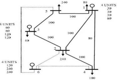
The TNEP model and the proposed method for solving it was implemented in MATLAB software and the TNEP algorithm was applied to the Garver's 6-bus network, shown in Fig. 2. Also, characteristics of the transmission lines are presented in Table 1 (Shariati et al., 2008). The total number of possible corridors for TNEP are considered in nine corridors out of which three corridors are new. The new corridors are shown by the dotted lines in Fig. 2. On the other hand, in order to consider uncertainty in the load, two scenarios—10% (first scenario) and 12% (second scenario)— have been predicted based on the scenario technique and by the same probability of occurrence for the load growth (Al-Saba & El-Amin, 2002). Theαcoefficient is assumed to be $10 million/MW. The planning horizon is 10 years and the network losses across each year of the planning horizon are determined (Shayeghi et al., 2008). Also in this paper, three expansion alternatives are suggested (see Table 2). The suggested alternatives with regard to the suggested prices by producers and the competitive power market mechanism, buying the maximum power from the plant, flatness of the Locational Marginal Prices (LMPs) in the network and the congestion reduction are experimentally achieved by the planner. So, without complicating the TNEP model, we can evaluate plans for different criteria such as congestion, price profile etc. The TNEP can be solved easily for large-scale systems. Also, for generating the alternatives, different methods can be used such as forward- and backward-expansion algorithms. Each algorithm will generate an alternative solution. The basic engineering concepts suggest using a lot of alternatives, so in this paper three different hybridization models are considered.

(7)

Table 1

Lines Data (X in P.U on 100 MVA BASE)

Investment cost (m$) Reactance (Ohm) Capacity (MW) To From Line N.O 2 0.4 100 2 1 1 6 0.6 80 4 1 2 2 0.2 100 5 1 3 1.5 0.2 100 3 2 4 4 0.4 100 4 2 5 2.5 0.2 100 5 3 6 3 0.3 100 6 2 7 3 0.3 100 6 4 8 6.1 0.3 78 6 5 9 Table 2

Proposed Alternatives for Network Expansion

Rights-of-Way Alternatives N.O

{2-6, 3-5, 4-6, 5-6} Alternative1

{2-6, 3-2, 4-6, 5-6} Alternative2

{2-6,1-2, 4-6, 5-6} Alternative3

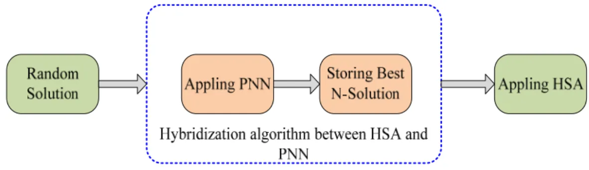
It should be noted that in practical power expansion, after determining the optimized plan, this plan is evaluated based on the stability and short-circuit-level limitations and whether the selected plan was determined unsuitable due to technical reasons, the planner should use the alternative plan. PNNs are also used for classifying the TNEP solutions. In this paper, the expansion solutions are four hybridizations of the total possible corridors, which total 126 states that were achieved. These states have been used for training and testing the PNNs. So, for training the PNNs, 80 different states were chosen out of the expansion solutions. The PNN output is one of the three suggested alternatives. Thus, the best n-solution set is produced. Then for every randomized input, the model selects the best n-solution set as an input for the HSA and, based on this, the network expansion is completed. Fig. 3 shows the hybridization algorithm between HSA and PNN. Since the number of layers and neurons are defined in a PNN, the only control parameter is core width (MATLAB Neural Network Toolbox User’s Guide, 1998). For determining it, the network error is evaluated based on the different core-width values. It should be noted that a small core core-width will increase the accuracy and sensitivity of the network and a large core width will improve the network generality. So, there should be a compromise between the network accuracy and its generality. The value of this variable was selected to be 0.9. Furthermore, the HSA algorithm parameters were set as follows: HMS = 8, HMCR = 0.85, PAR = 0.5 and bw=0.01.

Fig. 3. Hybridization algorithm between HSA and PNN

(8)

on first scenario are presented in Table 3. Fig. 4 shows the comparison of objective values for the first and second scenarios. As observed, the investment cost and the suggested first-alternative-losses cost is more suitable than the second and third alternatives and so the plan is more economical. The cost savings from considering the losses component is calculated by the difference in losses cost, before and after the expansion. Before the expansion, the losses cost for the test network is $135.36 million. So, for example for the first alternative according to the first scenario, the cost savings would be ($135.36m-$34.2m) = $101.16 million.

Table 3

Optimal plan and objectives values for the first scenario

Cost (million $) Lines

N.O Rights -of-Way

Alternative

N.O Saved

Cost Load not

Supply Active

Losses Investment

101.16 0

34.2 29.1

4 2-6

Alternative 1

2 3-5

2 4-6

1 5-6

98.46 0

36.9 28.6

4 2-6

Alternative 2

1 3-2

3 4-6

1 5-6

96.96 0

38.4 28.1

2 1-2

Alternative 3

4 2-6

2 4-6

1 5-6

Fig. 4. Comparison the objectives values for the first and second scenario

(9)

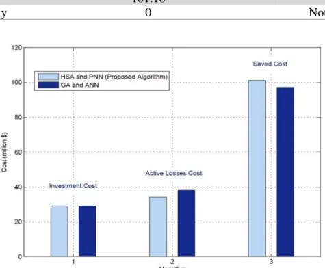
Table 4

Comparison of the objectives values with results similar to Al-Saba and El-Amin (2002)

Algorithms

Cost (million $) GA-ANN

Al-Saba and El-Amin (2002) HSA-PNN

Alternative1 (based on first scenario)

29.1 29.1

Investment

38.254 34.2

Active Losses

97.11 101.16

Saved Cost

Not Calculated 0

Load not Supply

Fig. 5. Comparison the objectives values with results similar to Al-Saba and El-Amin (2002)

6 Conclusion

In this paper, the transmission network expansion planning problem was analyzed using a new method in order to optimize the expansion costs, active losses costs and load. A hybridization model of the artificial intelligence tools was used to solve the TNEP. This model included a hybridization of the probabilistic neural networks and harmony search algorithm. Also, the suggested alternatives using the uncertainty role in the load were evaluated based on the expansion criteria. Based on the results, it was observed that the expansion plans are economical and effective.

References

Abdelaziz, A.R. (2000).Genetic algorithm based power transmission expansion planning. In:

Proceedings of the 7th IEEE international conference on electronics, Circuits and systems, 2,

642–645.

Al-Saba, T. & El-Amin, I. (2002). The application of artificial intelligent tools to the transmission expansion problem. International Journal of Electric Power Systems Research (Elsevier), 62, 117-126.

Binato, S., Oliveira, G.C. & Arajo, J.L. (2001). A greedy randomized adaptive search procedure for transmission expansion planning. IEEE Transactions on Power Systems, 16 (2), 247–53.

Choi, J., Tran, T., El-Keib, A. A., Thomas, R., Oh, H.S., & Billinton, R. (2005). A Method for Transmission System Expansion Planning Considering Probabilistic Reliability Criteria. IEEE

(10)

Christodoulou, C., & Georgiopoulos, M. (2001). Applications of Neural networks in

Electromagnetics. Artech House Publishers.

De, I., Silva, J., Rider, M.J., Romero, R., & Murari, C.A. (2005). Transmission network expansion planning considering uncertainness in demand. In: Proceeding of IEEE power engineering society

general meeting, 2, 1424-1429.

Eliassi, M., Seifi, H. & Haghifam, M.R. (2009). Multi-Objective Value-Based Reliability Transmission Planning Using Expected Interruption Cost Due to Transmission Constraint. Electric

Power and Energy Conversion Systems (EPECS '09), International Conference on 10-12, 1-8.

Latorre, G., Cruz, R. D., Areiza, J. M., & Villegas A. (2003). Classification of publications and models in transmission expansion planning. IEEE Transactions PWRS, 18, 938-946.

MATLAB Neural Network Toolbox User’s Guide, The MathWorks, 1998.

Sadegheih, A. & Drake, P.R. (2008). System network planning expansion using mathematical programming, genetic algorithms and tabu search. International Journal of Energy Conversion

and Management (Elsevier), 49, 1557–1566.

Shariati, H., Askarian Abyaneh, H. & Javidi, M. H. (2008). Transmission Expansion Planning Considering Security Cost under Market Environment. DRPT 2008 6-9 April 2008 Nanjing China, 1430-1435.

Shayeghi, H., Jalilzadeh, S., Mahdavi, M. & Haddadian, H. (2008). Studying influence of two effective parameters on network losses in transmission expansion planning using DCGA.

International Journal of Energy Conversion and Management (Elsevier), 49, 3017–3024.

Silva, I.J., Rider, M. J. & Romero, R. (2005). Transmission Network Expansion Planning Considering Uncertainty in Demand. IEEE Transactions on Power Systems, 21, 1565-1573.

Vasebi, A., Fesanghary, M. & Bathaee, S.M.T. (2007). Combined heat and power economic dispatch by harmony search algorithm. International Journal of Electrical Power and Energy Systems

(Elsevier), 29, 713–719.

Youseef, H. K. M. (2001). Dynamic transmission planning using a constrained genetic algorithm.