A Bag of Words Description Scheme for Image
Quality Assessment
Miguel Francisco Fidalgo Fernandes
Dissertação para obtenção do Grau de Mestre em
Engenharia Electrotécnica e de Computadores
(2º ciclo de estudos)
Orientador: Prof. Doutor António Manuel Gonçalves Pinheiro
tempo e que disponibilizou para que este trabalho fosse feito.
Ao Marco V. Bernardo, o aluno de doutoramento que tirou muitas das minhas dúvidas (algumas delas óbvias ou até ridículas).
Aos professores, de todos os ciclos de ensino desde o primário ao universitário, que permitiram que chegasse até aqui.
A todos os colegas de curso que se tornaram amigos, que conheci durante estes 5 anos. Aos colegas da minha banda, Semilunar, que me aturaram estes anos todos.
À família pelo seu apoio constante, avós, tios, primos e principalmente aos meus pais e à pirralha que chamo de irmã (ou talvez à irmã que chamo de pirralha).
e reproduzidas. Em qualquer destas operações podem ocorrer distorções que prejudicam a sua qualidade. A qualidade destas imagens pode ser medida de forma subjectiva, o que tem a desvantagem de serem necessários vários testes, a um número considerável de indivíduos para ser feita uma análise estatística da qualidade perceptual de uma imagem. Foram desenvolvi-das várias métricas objectivas, que de alguma forma tentam modelar a percepção humana de qualidade. Todavia, em muitas aplicações a representação de percepção de qualidade humana dada por estas métricas fica aquém do desejável, razão porque se propõe neste trabalho usar modelos de reconhecimento de padrões que permitam uma maior aproximação.
Neste trabalho, são dadas definições para imagem e qualidade e algumas das dificuldades do estudo da qualidade de imagem são referidas. É referida a importância da qualidade de imagem como ramo de estudo, e são estudadas diversas métricas de qualidade.
São explicadas três métricas, uma delas que usa a qualidade original como referência (SSIM) e duas métricas sem referência (BRISQUE e QAC). Uma comparação é feita entre elas, mostrando-– se uma grande discrepância de valores entre os dois tipos de métricas.
Para os testes feitos é usada a base de dados TID2013, que é muitas vezes considerada para estudos de qualidade de métricas devido à sua dimensão e ao facto de considerar um grande número de distorções. Neste trabalho também se fez um estudo dos tipos de distorção incluidos nesta base de dados e como é que eles são simulados.
São introduzidos também alguns conceitos teóricos de reconhecimento de padrões e alguns algoritmos relevantes no contexto da dissertação, são descritos como o K-means, KNN e as SVMs. Algoritmos de agregação de descritores como o “bag of words” e o “fisher-vectors” também são referidos.
Esta dissertação adiciona métodos de reconhecimento de padrões a métricas objectivas de qua– lidade de imagem. Uma nova técnica é proposta, baseada na divisão de imagens em células, nas quais uma métrica será calculada. Esta divisão permite obter descritores locais de qualidade que serão agregados usando “bag of words”. Uma SVM com kernel RBF é treinada e testada na mesma base de dados e os resultados do modelo são mostrados usando cross-validation. Os resultados são analisados usando as correlações de Pearson, Spearman e Kendall e o RMSE que permitem avaliar a proximidade entre a métrica desenvolvida e os resultados subjectivos. Este modelo melhora os resultados obtidos com a métrica usada e demonstra uma nova forma de aplicar modelos de reconhecimento de padrões ao estudo de avaliação de qualidade.
produced. All these operations can cause distortions that affect their quality. The quality of these images should be measured subjectively. However, that brings the disadvantage of achiev-ing a considerable number of tests with individuals requested to provide a statistical analysis of an image’s perceptual quality. Several objective metrics have been developed, that try to model the human perception of quality. However, in most applications the representation of human quality perception given by these metrics is far from the desired representation. Therefore, this work proposes the usage of machine learning models that allow for a better approximation. In this work, definitions for image and quality are given and some of the difficulties of the study of image quality are mentioned. Moreover, three metrics are initially explained. One uses the image’s original quality has a reference (SSIM) while the other two are no reference (BRISQUE and QAC). A comparison is made, showing a large discrepancy of values between the two kinds of metrics.
The database that is used for the tests is TID2013. This database was chosen due to its dimension and by the fact of considering a large number of distortions. A study of each type of distortion in this database is made.
Furthermore, some concepts of machine learning are introduced along with algorithms relevant in the context of this dissertation, notably, K-means, KNN and SVM. Description aggregator algorithms like “bag of words” and “fisher-vectors” are also mentioned.
This dissertation studies a new model that combines machine learning and a quality metric for quality estimation. This model is based on the division of images in cells, where a specific metric is computed. With this division, it is possible to obtain local quality descriptors that will be aggregated using “bag of words”. A SVM with an RBF kernel is trained and tested on the same database and the results of the model are evaluated using cross-validation.
The results are analysed using Pearson, Spearman and Kendall correlations and the RMSE to evaluate the representation of the model when compared with the subjective results. The model improves the results of the metric that was used and shows a new path to apply machine learning for quality evaluation.
Keywords
1 Introduction 1
2 Objectives and Scope 3
3 Image Quality 5
3.1 The pivotal necessity of Image Quality Assessment . . . 5
3.2 Definition of image quality metric . . . 5
3.3 Image Quality Assessment based on Error Sensitivity . . . 6
3.3.1 Framework . . . 7
3.3.2 Pre-Processing . . . 7
3.3.3 Constrast Sensitivity Filtering . . . 8
3.3.4 Channel Decomposition . . . 8
3.3.5 Error Normalization . . . 8
3.3.6 Error Pooling . . . 8
3.3.7 Evaluation of the Objective Models . . . 8
3.4 Image Metrics . . . 10
3.4.1 Structural Similarity Index Metric . . . 11
3.4.2 Quality Aware Clustering . . . 12
3.4.3 Blind/Referenceless Image Spatial QUality Evaluator . . . 14
3.4.4 Metrics Comparison . . . 15
3.5 TID2013 Database . . . 16
3.6 Types of Image Distortions . . . 18
3.6.1 Gaussian Noise . . . 18
3.6.2 High Frequency Noise . . . 21
3.6.3 Impulse Noise . . . 22
3.6.4 Quantization Noise . . . 22
3.6.5 Gaussian Blur . . . 23
3.6.6 Image Denoising . . . 23
3.6.7 Distortions in JPEG and JPEG200 . . . 24
3.6.8 Non-Eccentricity Pattern Noise . . . 24
3.6.9 Block-Wise Distortions of Different Intensity . . . 26
3.6.10 Mean Shift . . . 26
3.6.11 Contrast Changes . . . 27
3.6.12 Masked Noise . . . 27
3.6.13 Changes in Colour Saturation . . . 28
3.6.14 Comfort Noise . . . 28
3.6.15 Compression of Noisy Images . . . 28
3.6.16 Colour quantization . . . 29
3.6.17 Chromatic Aberrations . . . 29
4 Introduction to Machine Learning Concepts 33
4.1 Descriptors and Aggregation of Descriptors . . . 33
4.1.1 Bag of Words . . . 34
4.1.2 Fisher Vectors . . . 34
4.2 Classifiers . . . 34
4.2.1 Support Vector Machines . . . 35
4.3 Machine Learning applied to the Quality Evaluation . . . 36
5 Bag of Words Model Description Scheme for Image Quality Assessment 37 5.1 Local Image Quality Descriptors Computation . . . 37
5.2 Local descriptors aggregation using a Bag of Words . . . 37
5.3 Classification of the quality level of an image . . . 38
5.4 Training Selection . . . 39
5.5 Classification of an image bow quality descriptor using a Binary Support Vector Machine . . . 39
5.6 Analysis of Results for SSIM . . . 39
6 Comments and Future Work 49
Bibliografia 51
3.2 Comparison of Structural SIMilarity index (SSIM), Quality Aware Clustering (QAC) and Blind/Referenceless Image Spatial QUality Evaluator (BRISQUE) using the
Pear-son correlation coefficient . . . 16
3.3 Comparison of SSIM, QAC and BRISQUE using the Spearman rank order Correlation 16 3.4 Comparison of SSIM, QAC and BRISQUE using the Kendall rank order Correlation . 17 3.5 Comparison of SSIM, QAC and BRISQUE using the RMSE . . . 17
3.6 Reference Image 1 . . . 19 3.7 Reference Image 2 . . . 19 3.8 Reference Image 3 . . . 19 3.9 Reference Image 4 . . . 19 3.10 Reference Image 5 . . . 19 3.11 Reference Image 6 . . . 19 3.12 Reference Image 7 . . . 19 3.13 Reference Image 8 . . . 19 3.14 Reference Image 9 . . . 19 3.15 Reference Image 10 . . . 19 3.16 Reference Image 11 . . . 19 3.17 Reference Image 12 . . . 19 3.18 Reference Image 13 . . . 19 3.19 Reference Image 14 . . . 19 3.20 Reference Image 15 . . . 19 3.21 Reference Image 16 . . . 19 3.22 Reference Image 17 . . . 19 3.23 Reference Image 18 . . . 19 3.24 Reference Image 19 . . . 19 3.25 Reference Image 20 . . . 19 3.26 Reference Image 21 . . . 19 3.27 Reference Image 22 . . . 19 3.28 Reference Image 23 . . . 19 3.29 Reference Image 24 . . . 19 3.30 Reference Image 25 . . . 19
3.31 Reference Image for each distortion . . . 20
3.32 Additive Gaussian Noise. PSNR = 30dB. . . . 20
3.33 Additive Gaussian Noise. PSNR = 24dB. . . . 20
3.34 Additive White Gaussian noise added in colour components instead of in the lumi-nance component. PSNR = 30dB. . . . 20
3.35 Additive White Gaussian noise added in colour components instead of in the lumi-nance component. PSNR = 24dB. . . . 20
3.36 Additive Gaussian Spatially Correlated Noise. PSNR = 30dB. . . . 21
3.37 Additive Gaussian Spatially Correlated Noise. PSNR = 24dB. . . . 21
3.38 Multiplicative Gaussian Noise. PSNR = 30dB. . . . 21
3.40 Masked noise. PSNR = 30dB. . . . 21
3.41 Masked noise. PSNR = 24dB. . . . 21
3.42 High Frequency Noises. PSNR = 30dB. . . . 22
3.43 High Frequency Noises. PSNR = 24dB. . . . 22
3.44 Salt-and-Pepper Noise. PSNR = 30dB. . . . 22 3.45 Salt-and-Pepper Noise. PSNR = 24dB. . . . 22 3.46 Quantization Noise. PSNR = 30dB. . . . 23 3.47 Quantization Noise. PSNR = 24dB. . . . 23 3.48 Gaussian Blur. PSNR = 30dB. . . . 23 3.49 Gaussian Blur. PSNR = 24dB. . . . 23 3.50 Image Denoising. PSNR = 30dB. . . . 24 3.51 Image Denoising. PSNR = 24dB. . . . 24
3.52 JPEG lossy compression. PSNR = 30dB. . . . 25
3.53 JPEG lossy compression. PSNR = 24dB. . . . 25
3.54 JPEG2000 lossy compression. PSNR = 30dB. . . . 25
3.55 JPEG2000 lossy compression. PSNR = 24dB. . . . 25
3.56 JPEG lossy compression with transmission errors. PSNR = 30dB. . . . 25
3.57 JPEG lossy compression with transmission errors. PSNR = 24dB. . . . 25
3.58 JPEG2000 lossy compression with transmission errors. PSNR = 30dB. . . . 25
3.59 JPEG2000 lossy compression with transmission errors. PSNR = 24dB. . . . 25
3.60 Non-Eccentricity Pattern Noise. PSNR = 30dB. . . . 26
3.61 Non-Eccentricity Pattern Noise. PSNR = 24dB. . . . 26
3.62 Block-Wise Distortions of Different Intensity. PSNR = 30dB. . . . 26
3.63 Block-Wise Distortions of Different Intensity. PSNR = 24dB. . . . 26
3.64 Mean Shift. PSNR = 30dB. . . . 27
3.65 Mean Shift. PSNR = 24dB. . . . 27
3.66 Contrast Change. PSNR = 30dB. . . . 27
3.67 Contrast Change. PSNR = 24dB. . . . 27
3.68 Change in Colour Saturation. PSNR = 30dB. . . . 28
3.69 Change in Colour Saturation. PSNR = 24dB. . . . 28
3.70 Comfort Noise. PSNR = 30dB. . . . 29
3.71 Comfort Noise. PSNR = 24dB. . . . 29
3.72 Lossy Compression of Noisy Images. PSNR = 30dB. . . . 29
3.73 Lossy Compression of Noisy Images. PSNR = 24dB. . . . 29
3.74 Image colour quantization with dither. PSNR = 30dB. . . . 30
3.75 Image colour quantization with dither. PSNR = 24dB. . . . 30
3.76 Chromatic aberrations. PSNR = 30dB. . . . 30
3.77 Chromatic aberrations. PSNR = 24dB. . . . 30
3.78 Compressive sensing. PSNR = 30dB. . . . 31
3.79 Compressive sensing. PSNR = 24dB. . . . 31
5.1 Description Scheme. . . 38
5.2 Image quality classification. . . 38
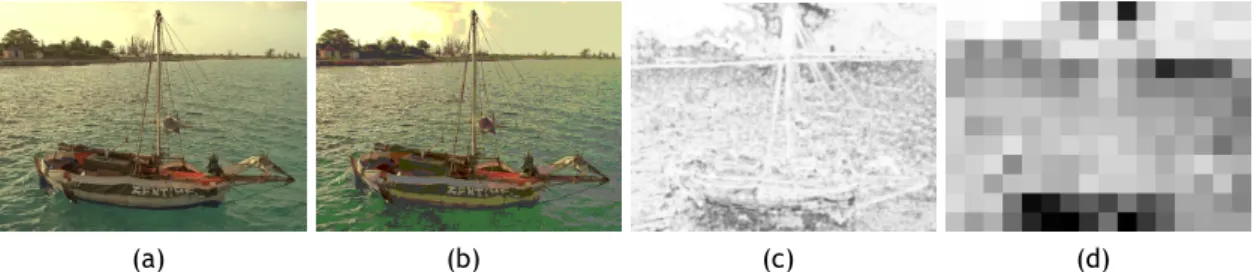
5.3 Example of Reference Image, Distorted Image, SSIM of entire image, and the mean SSIM outcome for the cell division (DCell = 32). . . . 39
5.4 Pearson correlation coefficient for 2× NCell bins Bag Of Words (BOW) boxplots for the ten fold cross-validation results. ’×’ marks the mean result. . . 40 xii
5.7 RMSE for 2× NCell bins BOW boxplots for the ten fold cross-validation results.
’×’ marks the mean result. . . 43
5.8 Pearson correlation coefficient comparing the SSIM, the 32:8:1 and the highest scoring combination for all distortion subsets for the ten fold cross-validation re-sults (mean result signalized by the ’×’). . . . 44 5.9 Spearman rank order correlation comparing the SSIM, the 32:8:1 and the
high-est scoring combination for all distortion subsets for the ten fold cross-validation results (mean result signalized by the ’×’). . . . 44 5.10 Kendall rank order correlation comparing the SSIM, the 32:8:1 and the highest
scoring combination for all distortion subsets for the ten fold cross-validation re-sults (mean result signalized by the ’×’). . . . 45 5.11 RMSE comparing the SSIM, the 32:8:1 and the highest scoring combination for all
distortion subsets for the ten fold cross-validation results (mean result signalized by the ’×’). . . . 45 5.12 Pearson correlation coefficient for different bow dimension (K of K-means) for
combinations 32:4:1 for the ten fold cross-validation results (mean result signal-ized by the ’×’). . . 46 5.13 Pearson correlation coefficient for different bow dimension (K of K-means) for
combinations 32:8:1 for the ten fold cross-validation results (mean result signal-ized by the ’×’). . . 46 5.14 Spearman correlation rank value for different bow dimension (K of K-means) for
combinations 32:4:1 for the ten fold cross-validation results (mean result signal-ized by the ’×’). . . 47 5.15 Spearman correlation rank value for different bow dimension (K of K-means) for
combinations 32:8:1 for the ten fold cross-validation results (mean result signal-ized by the ’×’). . . 47 5.16 Kendall correlation rank value for different bow dimension (K of K-means) for
combinations 32:4:1 for the ten fold cross-validation results (mean result signal-ized by the ’×’). . . 48 5.17 Kendall correlation rank value for different bow dimension (K of K-means) for
combinations 32:8:1 for the ten fold cross-validation results (mean result signal-ized by the ’×’). . . 48
5.1 Pearson correlation coefficient mean values. . . 40
5.2 Spearman rank order correlation mean values. . . 41
5.3 Kendall rank order correlation mean values. . . 42
BIQI Blind Image Quality Index BOW Bag Of Words
BPNN Back Propagation feed-forward Neural Network
BRISQUE Blind/Referenceless Image Spatial QUality Evaluator CBP Circular Back-Propagation
CSF Contrast Sensitivity Function
CWSSIM Complex Wavelet Structural SIMilarity index DCT Discrete Cosine Transform
FFNN Feed-Forward Neural Network FR Full Reference
FSIM Feature SIMilarity
HDTV High Definition Television HVS Human Visual System
IEEE Institute of Electrical and Electronics Engineers IPTV Internet Protocol Television
IQA Image Quality Assessment
MSCN Mean Subtracted Contrast Normalized MOS Mean Opinion Score
MSE Mean Squared Error KNN K-Nearest Neighbors MATLAB MATrix LABoratory NR No Reference
PSNR Peak Signal-to-Noise Ratio QAC Quality Aware Clustering QoE Quality of Service
QoMEX Quality Of Multimedia EXperience RBF Radial-Basis Function
RR Reduced Reference
SSIM Structural SIMilarity index SVM Support Vector Machine
WSSIM Wavelet based Structural SIMilarity index
Introduction
According to the dictionary1 an image is a representation of a physical likeness or
representa-tion of a person, animal or thing. Digital images are the result of the “acquisirepresenta-tion, processing, compression, storage, transmission and reproduction” [2] of that representation. The repre-sentations undergo all these forms of processing before they are ultimately displayed to a con-sumer. Every one of these processing steps alters the appearance of an image resulting in the need to assess impact on the final visual quality. Quality can be defined as “the perception, reflection about the perception and the description of an individual’s comparison and judg-ment process” [3]. There is, however, some misunderstanding and confusion of this term with “Beauty”.
“Beauty is in the eye of the beholder”. This famous phrase first appeared in the 3rd century BC in Greece. Famous writers like John Lyly, William Shakespeare, Benjamin Franklin and David Hume with slight changes have used it several times since. This old phrase couldn’t be more current and correct today. Its literal meaning is that the perception of beauty is subjective. However beauty is not quality. An individual could take a picture of a beautiful landscape with a camera of questionable performance and obtain a sub-par outcome. That photograph of something arguably pleasant to the human eye might have poor quality. The opposite could equally happen.
Knowing this, “can Image Quality be usefully quantified?” This line is the title of the first chapter of a book by Brian Keelan [4]. It summarizes the typical researchers’ struggle for the quality subjective prediction. That perception and interpretation of image quality can easily change from any person to another. Trying to predict the quality the average individual will evaluate an image on is an arduous task. Every one of the processing steps mentioned earlier alter the appearance of an image resulting in a need to assess the impact of processing on final visual quality.
1
Objectives and Scope
These days, with the high amount of handheld devices, social media and other electronic devices that display visual information it is of the most importance that the end-user has a satisfactory Quality of Service (QoE). Image quality, has perceived by humans, can be measured in a sub-jective way through subsub-jective tests. These tests have numerous disadvantages, namely long time sessions and the number of ratings per person required to achieve a reliable result. To avoid these disadvantages, objective metrics have been developed to simulate human behav-ior. These models objectively compute image quality and are later correlated to evaluate their performance. This dissertation addresses the need to use the knowledge about the human per-ceived quality. The goal of this work is to improve the typical values provided by metrics using the application of machine learning to image quality evaluation. A new technique is proposed based on the division of images into several cells where the mean of the SSIM metric is com-puted. A sliding window over a grid of cells that divide the image will define a set of image descriptors that are aggregated using a bag of words.
In Chapter 1 definitions for image and quality were given.
Chapter 3 considers why Image Quality Assessment (IQA) is important and gives a definition for “image metric” and how they are classified. A general framework for IQA systems is given. A classifications for Full Reference (FR) image metrics, are defined. Three metrics, SSIM, QAC and BRISQUE, are explained and a comparison between them is made. The image quality database that will be used is analyzed. Each distortion of the database is explained.
Chapter 4, introduces machine learning methods in the context of this dissertation and describes briefly algorithms like K-means clustering, K-Nearest Neighbors (KNN), Support Vector Machine (SVM)s and BOW.
The proposed approach will be described in the following chapter 5 along with the testing results using SSIM, and an analysis of the parameters influence.
Finally some conclusions and future research directions will be discussed in chapter 6.
The main conclusions of this work were published in the 2016 Eighth International Conference on Quality Of Multimedia EXperience (QoMEX) [5].
Image Quality
3.1
The pivotal necessity of Image Quality Assessment
IQA has, generally speaking, three kinds of applications [6] namely, to monitor image quality control systems, benchmarking image processing systems and algorithms and it’s embedding on image processing systems to optimize the algorithms and parameter settings.
An example of the first application could be an image and video acquisition system using a quality metric to monitor and automatically adjust itself to get the best image and video data quality possible. Another possible example would be a network video server. The digital video transmitted could have its quality examined and control the video streaming.
A second case example can be the continuous evaluation of several image processing systems, that require a certain image/video quality for a specific task.
Finally the third application can be exemplified by a visual communication system that uses a quality metric to improve the design of the pre-filtering and bit assignment algorithms at the encoder, and the post processing algorithms at the decoder.
With the proliferation of network handheld devices which can “capture, store, compress, send and display a variety of audiovisual stimuli like High Definition Television (HDTV), Internet Proto-col Television (IPTV) and websites such as Youtube and Facebook, an enormous amount of visual data is making its way to consumers” [7]. Due to this, there has been a considerable effort to ensure that the end users will be presented with a satisfactory QoE. According to QUALINET’s White Paper [3], “Quality of Experience is the degree of delight or annoyance of the user of an application or service. It results from the fulfillment of his or her expectations with respect to the utility and or enjoyment of the application or service in the light of the user’s personality and current state”. Since “the human eyes are the ultimate receivers in most image processing environments” [8], a subjective quality measurement Mean Opinion Score (MOS) of the system is the best indicator of how distortions affect perceived quality. The big disadvantage of doing this is the impracticality and time consumption needed to pool a large number of people to evaluate one or more images. Hence, models that somehow compute objectively the image quality and simulate the human behavior are required. Nevertheless, subjective assessment of visual quality is still used in all Image Quality databases to correlate with image quality metrics to analise it’s performances.
3.2
Definition of image quality metric
Image quality assessment aims to “use computational models (metrics) to measure the image quality consistently with subjective evaluations” [9].
Objective image quality metrics can be classified in three ways:
Full Reference - There is the assumption that an entire reference image is known, one of the
inputs is a pristine reference image with respect to which the quality of the distorted image is assessed;
No reference or “blind” quality assessment - No reference image is available. The only
in-formation that the algorithm receive before making a prediction is the distorted image whose quality is being assessed;
Reduced reference - When there is only a partial sample of the reference image or when the
algorithm possesses some information regarding the reference image, but not the actual reference image itself.
One of the first metrics was the Mean Squared Error (MSE), a full reference quality metric that consists in calculating the mean of the square root of the luminosity difference between the pixels of the distorted image and the pixels of the reference image. The MSE allows a comparison between the “true” pixel values for the original image and the noisy image representing the average of the squares of the “errors”.
MSE = 1 mn m∑−1 0 n∑−1 0 ∥f(i, j) − g(i, j)∥2 (3.1)
Peak Signal-to-Noise Ratio (PSNR) is an expression for the ratio between the maximum possi-ble value(power) of a signal and the power of distorting noise that affects the quality of its representation.
PSNR = 20log10(
M AXf
√
M SE) (3.2)
It is usually expressed in terms of the logarithmic decibel scale due to the wide dynamic range (ratio between the largest and smallest possible values of a changeable quantity). The higher the PSNR of an image, the more quality the degraded image has in comparison to the original. Common models like MSE and PSNR did not provide satisfying results when correlated with sub-jective results and the image quality researchers were forced to find other mechanisms that would enhance the outcome when compared to its subjective equivalents [10].
Modern IQA algorithms estimate quality using a variety of image analysis techniques. When a reference image is available, local differences between the reference and distorted images are measured in various domains, and such differences are mapped for quality estimation.
3.3
Image Quality Assessment based on Error Sensitivity
Computational models for IQA have been developed by exploring effective features that are consistent with the characteristics of a Human Visual System (HVS) for visual quality perception. An image signal that is being subjected to an image metric can be considered as the sum between an undistorted image signal and an error signal [1]. IQA models are necessary because two distorted images that have the same MSE can have distinct errors that can be more or less visible than others. This is due to the fact that the MSE can only quantify the intensity of the error signal [1]. We can conclude from this that a perceptual loss of image quality isn’t at all related to the visibility of the error signal. Most IQA approaches are related with error sensitivity aspects like visibility.
Figure 3.1: Prototype of an Image Quality Assessment System based on Error Sensitivity [1]
The system is comprised of Pre-Processing, Contrast Sensitivity Function (CSF) Filtering, Channel Decomposition, Error Normalization, Error Pooling and Quality measurement [1]. The CSF fea-ture may be implemented separately, as displayed in the scheme, or in the Error Normalization stage.
3.3.2
Pre-Processing
This phase consists in basic operations devised to eliminate known distortions from the images that will be processed.
Firstly, if the images to be compared don’t have the same size, they are scaled and aligned. The used signals will, also, be beforehand converted from the RGB colour values to Y CbCr colour space. This transformation is done because it is perceived that Y CbCr is more appropri-ate for comparisons relappropri-ated with the HVS. RGB is an additive colour model in which red, green and blue light are added together to reproduce a broad array of colours. RGB signal are not efficient as a representation for storage and transmission, since they have a lot of redundancy.
Y CbCris a practical approximation to colour processing and perceptual uniformity, where the
primary colours (red, green and blue) are processed into perceptually meaningful information.
Y CbCris used to separate out the luminance component (Y ) and two Chroma components (Cb
and Cr). With this conversion the Y channel is typically used as the metric input, and the Chroma components are in many cases just ignored.
The quality assessment metrics may need to convert the values of the digital pixels, stored in the computer memory in luminance values on the display device, using a linear point-wise transformation.
A low-pass filter simulating a point-spread function can be applied.
Finally, both images can be modified using a nonlinear point operation to simulate light adap-tation.
3.3.3
Constrast Sensitivity Filtering
The CSF measures the threshold sensitivity of the HVS over a wide range of different spatial and temporal frequencies [11]. Some image quality metrics include a stage that analyses the signal according to this function, playing a central role in image processing techniques like compres-sion. It is normally performed by applying a linear filter that estimates the response frequency of the CSF [1]. Nonetheless, other metrics also apply CSF after the channel decomposition as a base sensitivity normalization factor.
3.3.4
Channel Decomposition
In this stage images are divided into channels depending on their spatial frequencies, temporal frequencies or their orientation [1]. Whilst some methods of quality assessment implement sophisticated channel decomposition, others just apply a Discrete Cosine Transform (DCT) or separate the signal bands using wavelet transforms.
3.3.5
Error Normalization
This stage computes the difference between the reference and the distorted for each channel that was decomposed in the previous stage, followed by their normalization using a mask. If two or more image components have similar spatial frequencies, temporal frequencies or orienta-tions, this process will decrease their visibility [1]. The difference is calculated by subtracting the intensity of the reference and the distorted coefficients of the same channel within a spatial neighborhood. Some methods also consider the effect of contrast response saturation.
3.3.6
Error Pooling
This final step is where a single value, that classifies the image quality objectively is obtained. All the different channels previously obtained, along with the normalized error signals, are pooled together. On most metrics, the pooling takes the shape of a Minkowsky norm [1],
E({el,k}) = ( ∑ l ∑ k |el,k| β )1/β (3.3)
where el,kis the normalized error of the K-th coefficient of the l-th channel and β is a
exponen-tial constant typically chosen between 1 and 4. Minkowsky pooling can be done is space(index
k) and after in frequency (index l) or vice-versa, with some non-linearity between them, or pos-sibly with different β. A spatial map can indicate the relative importance of different regions and what can be used to obtain variant spatial weighting.
3.3.7
Evaluation of the Objective Models
To evaluate the performance of a metric, the Pearson correlation coefficient, Spearman rank order correlation, Kendall rank order correlation and the RMSE, between the subjective MOS and the quality estimation, are used.
MOSp= b1 +
b2
1 + e(−b3(MR−b4)) (3.4)
The values of the MOS associated an image are normalized according to equation 3.5 where
M R is the result of our methodology and b1, b2, b3 and b4 denote the regression parameters, initialized with M OSmin, M OSmax, M Rmin and M Rmaxrespectively,
MOSn(i) = 5×
MOS(i)− MOSmin
MOSmax− MOSmin
(3.5)
3.3.7.2 Pearson Linear Correlation
The Pearson linear correlation coefficients rP measures the model prediction accuracy.
rP = ∑N j=1(Sj− ¯S)(Oj− ¯O) √∑N j=1(Sj− ¯S)2( ∑N j=1Oj− ¯O)2 (3.6)
In this case, Sj denotes the subjective score M OSn and Oj the objective M OSp. ¯Sand ¯O are
the means of the respective data sets and N represents the total number of image samples considered in the analysis.
3.3.7.3 Spearman Rank-Order Correlation
The Spearman rank-order correlation coefficient rS evaluates the model prediction
monotonic-ity.
rS= 1− (
6∑Nj=1d2j
N (N2− 1)) (3.7)
where d is the difference between the ranked M OSn and the ranked M OSp. In practice, this
is computed as the Pearson correlation, but instead of the variables the ranked variables are used. N represents the total number of image samples considered in the analysis.
3.3.7.4 Kendall Rank-Order Correlation
Kendall rank correlation rK is a non-parametric test that measures the strength of dependence
between two variables [12].
rK =
Nc− Nd
1
2N (N − 1)
(3.8)
where Nc is the number of concordant pairs [12], Nd is the number of discordant pairs and N
3.3.7.5 Root Mean Square Error
RMSE measures the quality prediction error that is maximized when the RMSE is minimized.
RM SE =
√∑N
j=1(Sj− OJ)2
N (3.9)
where N represents the total number of image samples considered in the analysis.
3.4
Image Metrics
Numerous objective methods for image evaluation have been introduced over the years from the first ones like MSE and PSNR (previously mentioned) to the more recent metrics. These met-rics, as it has been previously noted, can be FR, No Reference (NR) or Reduced Reference (RR). The FR quality assessments can be divided in different categories: difference measures and statistical-oriented metrics, structural similarity measures, visual information metrics, infor-mation weighted metrics, HVS-inspired metrics and colour difference metrics.
Difference Measures and Statistical-Oriented Metrics - These metrics are based on pixel
val-ues differences and provide measures between the reference and the distorted image. Two examples of this category are the MSE and the PSNR.
Structural Similarity Measures- These metrics model the quality based on pixel statistics to
model the luminance (using the mean), the contrast (variance), and the structure (cross-correlation).
Visual Information Measures - These metrics aim at measuring the image information by
mod-eling the psycho-visual features of the HVS or by measuring the information fidelity. Then, the models are applied to the reference and distorted image, resulting in a measure of the difference between them.
Information Weighted Metrics - The metrics in this category are based on the modeling of
rel-ative local importance of the image information. As not all regions of the image have the same importance in the perception of distortion, the image differences computed by any metrics have allocated local weights resulting in a more perceptual measure of quality.
HVS Inspired Metrics - These metrics try to model empirically the human perception of images
from real scenes.
Colour Difference Measures - The colour difference metrics were developed because the CIE1976
colour difference magnitude in different regions of the colour space did not appear cor-related with perceived colours.
One of the most impactful FR quality metric SSIM. It is a method that improved upon earlier metrics such as PSNR and MSE. The 2004 paper in which it is described[1] is one of the most cited papers in image processing and was even awarded the Institute of Electrical and Electronics Engineers (IEEE) Signal Processing Society Best Paper Award1. This metric will be used later in
the algorithm proposed in this dissertation.
1http://signalprocessingsociety.org/uploads/awards/Best_Paper.pdf
3.4.1
Structural Similarity Index Metric
The SSIM [1] is an objective metric based on the degradation of structural similarity. SSIM is based on that assumption that the HVS extracts structural information from the analyzed image textures. The SSIM index incorporates three representative features for luminance, contrast and structural information that are extracted by the average pixel intensity values, the stan-dard deviation of the local image regions and the cross correlation values between two local image regions and the cross correlation values between two local image regions, respectively. Supposing x and y are two non-negative image signals, with one being the reference image and the other the distorted image, the luminance of each signal is compared:
µ = 1 N N ∑ i=1 xi (3.10)
The luminance comparison function l(x, y) is a function of µx and µy. The signal contrast is
calculated as described earlier:
σx= ( 1 N− 1 N ∑ i=1 (xi− µx)2)1/2 (3.11)
The contrast comparison c(x, y) is then the comparison of σxand σy. The signal comparison is
then normalized(divided) by its own standard deviation. The structure comparison is conducted on these normalized signals (x− µx)σxand (y− µy)σy.
The three components are combined resulting is an overall similarity measure:
S(x, y) = f (l(x, y), c(x, y), s(x, y)) (3.12)
These three components are relatively independent from each other. For luminance comparison:
l(x, y) = 2µxµy+ C1
µ2
x+ µ2y+ C1
(3.13)
where the constant C1 is included to avoid instability when µ2x+ µ2y is approximately zero. C1
is defined as
C1= (K1∗ L)2 (3.14)
where L is the dynamic range of the pixel values (255 for 8-bit grayscale images) and K1<< 1is
a small constant. Weber’s law says that the magnitude of a just-noticeable luminance change δ I is approximately proportionate to the background luminance I for a wide range of luminance values. This means that the HVS is sensitive to relative luminance changes and it is not to absolute luminance change. Applying Weber’s law on the luminance equation,we can rewrite
luminance. Substituting in Eq. :
l(x, y) = 2(1 + R)
1 + (1 + R)2+ C 1/µ2x
(3.15)
The contrast function is similar to the luminance function:
c(x, y) = 2σxσy+ C2
σ2
x+ σ2y+ C2
(3.16)
where C2= (K2L)2andK2 << 1. The structural comparison is done after luminance subtraction
and variance normalization.
s(x, y) = σxy+ C3
σxσy+ C3
(3.17)
In the discrete form, σxycan be estimated as:
σxy= 1 N− 1 N ∑ i=1 (xi− µx)(yi− µy) (3.18)
Combining the three equations:
SSIM (x, y) = [l(x, y)]α× [c(x, y)]β× [s(x, y)]γ (3.19)
where α > 0, β > 0 and γ > 0 are parameters that adjust the relative importance of each component. To simplify the expression α = β = γ = 1 and C3 = C2/2resulting in a specific
form of the SSIM index:
SSIM (x, y) = (2µxµy+ C1)(2σxy+ C2)
(µ2
x+ µ2y+ C1)(σx2+ σ2y+ C2)
(3.20)
3.4.2
Quality Aware Clustering
QAC [13] is a RR metric for general purpose Blind Image Quality Assessment (BIQA). The metric is built upon a set of some reference and distorted images (but without human score), divide the distorted images into overlapped cells and use a percentile pooling strategy to estimate the local quality level of each patch. Then the QAC method is proposed to learn a set of centroids on each quality level. These centroids are to obtain the quality of each cell in a given image, using a nearest neighbor algorithm, and subsequently a perceptual quality score of the whole image can be obtained.
3.4.2.1 Learning of Quality-Aware Centroids by QAC
First, there is a Random selection of 10 source images from the Berkeley Image Database [14] due to them having different scenes from the images in the databases. Each image is distorted to obtain the four of the most common types of distortions: Gaussian noise, Gaussian blur, JPEG compression and JPEG2000 compression. There are three quality levels for each of the four distortions to make sure that the quality distribution of the resulted samples that will be obtained is balanced.
The distortion level is controlled as in the following, standard deviation for Gaussian noise, blur kernel for Gaussian Blur, compression ratio for JPEG and JPEG2000.
a FR IQA similarity function such as SSIM [1] previously mentioned or Feature SIMilarity (FSIM) [9] to calculate the similarity between xi and di. This way, there will be no dependency of human
scores. The FSIM’s formula is
si= S(xi, di) = 2P C(xi)P C(di) + t1 P C(xi)2+ P C(di)2+ t1× 2G(xi)G(di) + t2 G(xi)2+ G(di)2+ t2 (3.21)
where P C(xi)and G(xi)refer to the phase congruency and gradient magnitude at the center
of xi, respectively, and t1 and t2are positive constants for numerical stability.
Each cell(dy ) will have a similarity score between 0 and 1. The si’s are normalized using a
percentile pooling procedure [13] to obtain an average close to the overall perceptual quality. In particular, si is divided by a constant C to define an average quality of all patches in an
image will equal to the percentile pooling result. Denoting with Ω as the set of patch indices of an image, and by Ωp the set of indices of the 10% percentile results with the lowest quality
patches. The normalization factor C is calculated as:
C =
∑
iΩsi
10∑iΩpsi
(3.22)
After that, each si is normalized as: ci= si/C.
With the cell quality normalization strategy, we acquire a set of cells di and their normalized
scores ci, on which the quality-aware clustering can be executed. Using ci, di can be grouped
into groups of similar quality obtaining different clusters based on local structures. Because ci
is a real-value number between 0 and 1, firstly ciis uniformly quantized into L levels, denoted
by ql= l/L, l = 1, 2, ..., L. The cells that have the same quality are then grouped into the same
group, denote by Gl. Gl= di|ci6 ql, for l = 1 di|ql−1< ci< ql, for l = 2, ..., L (3.23)
The clustering is then applied to each group Gl. To enhance the clustering accuracy, the QAC
within each Glshould be based on some structural feature of di. The following high pass filter
to extract the feature of cell di:
hσ(r) = 1r=0− 1 √ 2πσexp(− r2 2σ2) (3.24)
where σ is the scale parameter to control the shape of the filter. By convolving hσ with the
image, the image’s detailed structures will be enhanced. Three hσare used on different scales
(σ = 0.5, 2.0, 4.0) to extract the feature of di. The filtering outputs of dion the three scales are
concatenated into a feature vector, denoted by fi. The acQAC of diεGl is then performed by
minml,k K ∑ k=1 ∑ diεGl,k ∥fi− ml,k∥ 2 (3.25)
where Gl,kis the kthcluster in Group Gl. The Euclidean distance is used as the similarity metric
due to complexity costs.
3.4.2.2 Performing Blind Quality Estimation
To perform blind quality pooling, using the learned quality-aware centroids ml,k, one must go
through the following stages: patch partition and feature extraction, cluster assignment on multiple levels, patch quality estimation and final pooling with all patches’ quality.
Patch partition and feature extraction- Each test image is partitioned into N overlapped patches
yi and use high pass filters hσ to extract the feature vector, denoted by fiy, of each yi, i = 1, ..., N.
Cluster assignment- Find the nearest centroid to the feature vector fiy of patch yiby assuming
that patches which have similar structural features will have similar visual quality.
Patch quality estimation- The distance between fiyand ml,kiis δl,i=∥f
y
i − ml,k∥
2
. The shorter the distance σl,k is, the more likely patch yishould have the same quality level as that of
centroid ml,ki. Therefore, we can use the following weighted average rule to determine
the final quality score of yi:
zi= ∑L l=1qlexp(−δl,i/λ) ∑L l=1exp(−δl,i/λ) (3.26)
where λ is a parameter to control the decay rate of weight exp(−δl,i/λ)with reference to
distance δl,i.
Final pooling Using the estimated quality zi of all patches yi, the final single quality score,
denoted by z of the test image, y is obtained. The pooling is done using the following equation: z = 1 N N ∑ i=1 zi (3.27)
3.4.3
Blind/Referenceless Image Spatial QUality Evaluator
BRISQUE [7] is also a RR metric.
The metric starts by computing normalized luminances in a distorted image using local mean subtraction and divisive normalization.
(i, j) = (I(i, j)− µ(i, j))/(σ(i, j) + C) (3.28)
where, iε1, 2...M , jε1, 2...N are spatial indices, M , N are the image height and width respec-tively, C = 1 is a constant that prevents divisions by 0 and
and σ(i, j) = v u u t ∑K k=−K L ∑ l=−L ωk,l(Ik,l(i, j)− µ(i, j))2 (3.30)
where ωk,l|k=−K,...,K,l=−L,...,Lis a 2D circularly-symmetric Gaussian weighting function sampled
out to 3 standard deviations and rescaled to unit volume. K and L are constants equal to 3. The transformed luminances are refered as Mean Subtracted Contrast Normalized (MSCN) coefficients.
Also, the statistical relationships between neighboring pixels are modeled according to four orientation (horizontal (H), vertical (V ), main-diagonal (D1) and secondary diagonal(D2)).
H(i, j) = (i, j)(i, j + 1) (3.31)
V (i, j) = (i, j)(i + 1, j) (3.32)
D1(i, j) = (i, j)(i + 1, j + 1) (3.33)
D2(i, j) = (i, j)(i + 1, j− 1) (3.34)
for i ε 1, 2...M and j ε 1, 2...N
For each of the four orientations, four parameters are computed (shape, mean, left variance and right variance) using a GGD [7] obtaining 16 values which will be part of the feature. The feature has now 18 values. The original distorted image is filtered using a low-pass filter and is downscaled by a factor of 2. Another 18 values are extracted. The final BRISQUE feature has 36 values.
The metric uses a SVM with a Radial-Basis Function (RBF) kernel that was previously trained using the LIVE database to obtain a quality evaluation. The input for each image is the feature previously calculated.
3.4.4
Metrics Comparison
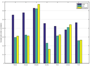
The three detailed metrics of previous section, SSIM, QAC and BRISQUE, were compared to evaluate the path to follow in this dissertation. The Pearson, Spearman, Kendall correlations, and also the RMSE between this three metrics and the MOS given in figures 3.2, 3.3, 3.4 and 3.5, reveal that the NR metrics are still far from providing an appropriate representation. The SSIM reveal always an improved estimation, apart the case of the simple and colour distortions classes. For this reason, during this work these metrics have been not used, and only SSIM was considered. Of course, other FR metrics could be used but from our preliminary tests no different conclusions should be defined.
Noise Actual Simple Exotic New Colour Full 0 0.1 0.2 0.3 0.4 0.5 0.6 0.7 0.8 0.9
Pearson rank order corr
SSIM QAC BRISQUE
Figure 3.2: Comparison of SSIM, QAC and BRISQUE using the Pearson correlation coefficient
Noise Actual Simple Exotic New Colour Full 0 0.1 0.2 0.3 0.4 0.5 0.6 0.7 0.8 0.9
Spearman rank order correlation
SSIM QAC BRISQUE
Figure 3.3: Comparison of SSIM, QAC and BRISQUE using the Spearman rank order Correlation
3.5
TID2013 Database
The database used for training and testing is the TID2013 [2]. This database contains images with 24 different distortion types. Each type has five levels of distortion. For all types of dis-tortions the corresponding levels of PSNR are of about 33dB, 30dB, 27dB, 24dB and 21dB (Lv1, Lv2, Lv3, Lv4 and Lv5). According to the creators of the database, this number of distortions for the 25 reference images is enough to reliably cover the full range of subjective quality. There were made subjective experiences in five countries to obtain a MOS. All the distorted images were obtained from the Kodak database2with the exception of one image (synthetic) that was
artificially created.Each reference image originates 120 distorted images (five levels for each of twenty four types of distortions). The images have a fixed dimension of 384×512 pixels for unifi-cation purposes. The distortion types present in the database are Additive White Gaussian Noise
2
r0k.us/graphics/kodak/
Noise Actual Simple Exotic New Colour Full 0 0.1 0.2 0.3 0.4
Kendal rank order correlation
Figure 3.4: Comparison of SSIM, QAC and BRISQUE using the Kendall rank order Correlation
Noise Actual Simple Exotic New Colour Full 0 5 10 15 20 25 30 35 40 45 RMSE SSIM QAC BRISQUE
Figure 3.5: Comparison of SSIM, QAC and BRISQUE using the RMSE
applied to the luminance component (#1), Additive White Gaussian Noise applied to the colour components (#2), Spatially Correlated Additive Gaussian Noise (#3), Masked Noise (#4), High Fre-quency Noise (#5), Impulse Noise (#6), Quantization Noise (#7), Gaussian Blur (#8), Image Denois-ing (#9), JPEG Lossy Compression (#10), JPEG2000 Lossy Compression (#11), JPEG Transmission Errors (#12), JPEG2000 Transmission Errors (#13), Non-Eccentricity Pattern Noise (#14), Local Block-Wise Distortions of Different Intensity (#15), Mean Shift (#16), Contrast Change (#17), Change of Colour Saturation (#18), Multiplicative Gaussian Noise (#19), Comfort Noise (#20), Lossy Compression of Noisy Images (#21), Image Colour Quantization with Dither (#22), Chro-matic Aberrations (#23), Sparse Sampling and Reconstruction (#24). The distortion types were divided in subsets, to allow an improved analysis of the data.
Table 3.1: Distortion subsets
No. Type of Distortion Noise Actual Simple Exotic New Colour Full
1 Additive White Gaussian Noise + + + - - - +
2 Noise in Colour Comp. + - - - - + +
3 Spatially Correl. Noise + + - - - - +
4 Masked Noise + + - - - - +
5 High Frequency Noise + + - - - - +
6 Impulse Noise + + - - - - + 7 Quantization Noise + - - - - + + 8 Gaussian Blur + + + - - - + 9 Image Denoising + + - - - - + 10 JPEG Compression - + + - - + + 11 JPEG2000 Compression - + - - - - +
12 JPEG Transm. Error - - - + - - +
13 JPEG2000 Transm. Errors - - - + - - +
14 Non Ecc. Patt. Noise - - - + - - +
15 Local Block-Wise - - - + - - +
16 Mean Shift - - - + - - +
17 Contrast Change - - - + - - +
18 Change of Colour Saturation - - - - + + +
19 Multiplicative Gaussian Noise + + - - + - +
20 Comfort Noise - - - + + - +
21 Lossy Compression Noisy Images + + - - + - +
22 Image Colour Quantization w/ Dither - - - - + + +
23 Chromatic Aberrations - - - + + + +
24 Sparse Sampling and Reconstruction - - - + - - +
3.6
Types of Image Distortions
This section gives a definition to each distortion, explains how each one is obtained and shows their effect on a specific reference image 3.31.
3.6.1
Gaussian Noise
In general, noise is an unwanted component in an image. Any degradation, such as a random variation of brightness or colour information that occurs in an image, can be called noise [15]. The most common form of noise is the so-called Additive noise, can be defined as:
f = g + q (3.35)
where f is an image and g and q are the original image and the noise component, respectively. Some less common noises are multiplicative, instead of additive, resulting,
f = g× q (3.36)
Multiplicative noise can be changed into an additive model by using the logarithmic function:
ef = eg+q= efeq (3.37) 18
Figure 3.6: Reference Image 1 Figure 3.7: Reference Image 2 Figure 3.8: Reference Image 3 Figure 3.9: Reference Image 4 Figure 3.10: Reference Image 5 Figure 3.11: Reference Image 6 Figure 3.12: Reference Image 7 Figure 3.13: Reference Image 8 Figure 3.14: Reference Image 9 Figure 3.15: Reference Image 10 Figure 3.16: Reference Image 11 Figure 3.17: Reference Image 12 Figure 3.18: Reference Image 13 Figure 3.19: Reference Image 14 Figure 3.20: Reference Image 15 Figure 3.21: Reference Image 16 Figure 3.22: Reference Image 17 Figure 3.23: Reference Image 18 Figure 3.24: Reference Image 19 Figure 3.25: Reference Image 20 Figure 3.26: Reference Image 21 Figure 3.27: Reference Image 22 Figure 3.28: Reference Image 23 Figure 3.29: Reference Image 24 Figure 3.30: Reference Image 25
The opposite can also be done
log(f ) = log(g× q) = log(g) + log(q) (3.38)
Some noises can be described in an easier way using additive models, while others are better described as multiplicative models. Additive White Gaussian Noise (#1) is the most common occurring noise [15]. This type of noise follows a Gaussian distribution, meaning that it’s prob-ability density function given by the normal distribution (or Gaussian distribution).
Pq(x) = 1 √ 2πσ2e −(x−µ)2 2σ2 f or− ∞ < x < ∞ (3.39)
Figure 3.31: Reference Image for each distortion
Figure 3.32: Additive Gaussian Noise. PSNR = 30dB.
Figure 3.33: Additive Gaussian Noise. PSNR = 24dB.
Figure 3.34: Additive White Gaussian noise added in colour components instead
of in the luminance component. PSNR = 30dB.
Figure 3.35: Additive White Gaussian noise added in colour components instead
of in the luminance component. PSNR = 24dB.
Figures 3.32 and 3.33 and shows how the distortion affects the reference image.
In the second distortion instead of adding the noise to the luminance component Y , the noise is added to the colour components CbCr using a gaussian distribution [16]. An example with two different quality levels can be seen in 3.34 and 3.35. This distortion was added to test if quality metrics perceive brightness (luminance) and colour (chrominance) differently just like the HVS does.
The third distortion is also additive gaussian noise, but this time being a low-pass spatially correlated noise [2]. To obtain this distortion, noise is generated and then filtered using a low-pass filter. The result is added to the reference image.
Multiplicative Gaussian Noise (#19) is Gaussian noise that follows the multiplicative model ex-plained above, instead of the additive one. In this database, before multiplying the Gaussian 20
Figure 3.36: Additive Gaussian Spatially Correlated Noise. PSNR = 30dB.
Figure 3.37: Additive Gaussian Spatially Correlated Noise. PSNR = 24dB.
Figure 3.38: Multiplicative Gaussian Noise. PSNR = 30dB.
Figure 3.39: Multiplicative Gaussian Noise. PSNR = 24dB.
Figure 3.40: Masked noise. PSNR = 30dB. Figure 3.41: Masked noise. PSNR = 24dB.
noise with the reference image, the noise was simulated separately for each RGB colour with equal σ2 (variance) [2]. The results can be observed in 3.38 and 3.39.
3.6.2
High Frequency Noise
Noise fluctuations can vary in spatial frequency3. High frequency images have a finer texture,
as can be seen in figures 3.42 and 3.43, while a low frequency image has a coarser texture. High Frequency Noise(#5) is related to the spatial frequency of HVS [17]. The distorted image can be obtained by generating white noise followed by a high pass filter.
3
Figure 3.42: High Frequency Noises. PSNR = 30dB.
Figure 3.43: High Frequency Noises. PSNR = 24dB.
Figure 3.44: Salt-and-Pepper Noise. PSNR = 30dB.
Figure 3.45: Salt-and-Pepper Noise. PSNR = 24dB.
3.6.3
Impulse Noise
The #6 distortion is Impulse Noise. Also called salt-and-pepper noise, images with this type of noise have dark pixels in brighter regions and bright pixels in darker regions. These distorted images appear to have black and white “dots” (salt-and-pepper). These outliers can be caused by bit errors in transmission or errors in analog-to-digital conversion [15]. When each pixel is quantized into B bits, it’s value X can be written as,
X =
B∑−1
i=0
bi2i (3.40)
Assuming a binary symmetric channel with a crossover probability P R equal to ε, flipping each bit with the same probability and defining the received value as Y , the probabilities can be expressed as:
P r(|X − Y | = 2i) = εfor i = 0, 1, ..., B− 1 (3.41)
The pixels with the most changed bits should appear as black or white “dots”.
3.6.4
Quantization Noise
Quantization Noise (#7) is caused when quantizing the pixels of a sensed image to a discrete number or number of discrete levels [15]. A continuous image signal is converted into a dis-22
Figure 3.46: Quantization Noise. PSNR = 30dB.
Figure 3.47: Quantization Noise. PSNR = 24dB.
Figure 3.48: Gaussian Blur. PSNR = 30dB. Figure 3.49: Gaussian Blur. PSNR = 24dB.
crete digital representation where a range of input values produces the same output producing discrete, stepped digital data resulting in a slight error. This distortion has an approximately uniform distribution and usually occurs in the acquisition process. The image’s previous smooth gradations become regions separated by noticeable discontinuities.
3.6.5
Gaussian Blur
Gaussian Blur (#8) is a blur effect that occurs when an image is acquired during a motion/shaking period that smooths the image’s sharpness (edges and boundaries) [18]. The visual effect of this blurring technique is a smooth blur similar to seeing the image through a translucent screen. It can be modeled as the result of blurring an image by a Gaussian filter. The MATrix LABoratory (MATLAB) function “imgaussfilt” can perform this transformation by applying the convolution kernel to the image:
g(x, y) = 1
2πσ2e
−x2 +y2
2σ2 (3.42)
where x and y are the pixel’s location and σ is the standard deviation of the Gaussian Blur. It is often used as a pre-processing stage in computer vision algorithms in order to enhance image structures at different scales. Gaussian smoothing is very frequently used with edge detection.
3.6.6
Image Denoising
The #9th distortion is Image Denoising. There have been some efforts in trying to recover distorted images using denoising algorithms (filters) [19]. The resulting images may still contain
Figure 3.50: Image Denoising. PSNR = 30dB.
Figure 3.51: Image Denoising. PSNR = 24dB.
residual distortions that eventually look perceptually worse as bad quality [16]. The images in this database had Gaussian noise that was filtered using a acDCT [20]. The colour channels of the noisy image are descorrelated. The DCT technique decomposes the image into local cells of same size. The article [21] arques that a 16× 16 window leads to the best results. A DCT transform is calculated for each cell, it’s coefficients and thresholded (with a threshold equal to 3σ and an inverse DCT tranform is then calculated. Finally, the cells are averaged and aggregated to reconstruct the denoised image.
3.6.7
Distortions in JPEG and JPEG200
Compression is a data transformation followed by an enconding method [22] used to decrease the data file’s size. While in lossless image compression, the goal is to represent an image using the least amount of bits without loss of information, in lossy image compression the goal is to achieve a faithful representation of the image using the least amount of bits [15]. It is clear that in lossy image compression there is some loss of information. The advantage of this method though, is the reduction of the image’s size and bit-rate. The results of coding and decoding the image with JPEG (#10) and JPEG2000 (#11) with different degrees of compression can be seen in figures 3.52, 3.53, 3.54 and 3.55, respectively.
Moreover, and in the addition to the CODEC processes, transmission networks can add error to the streaming data. Distortions 12 and 13 show respectively the result of adding randomly bit errors to the encoded JPEG and JPEG2000 data stream of the images, resulting in decoding errors. The results can be observed in 3.56 and 3.57 (#12) and 3.58 and 3.59 (#13).
3.6.8
Non-Eccentricity Pattern Noise
Humans have difficulty in perceiving an image’s distorted fragments if they appear similar to the original texture or the colour of the surrounding fragments. For this reason, the Non-Eccentricity Pattern Noise distortion (#14) was created and modeled for this database. Blocks of 15x15 pixels were randomly taken from the reference image and copied to locations of another blocks nearby. Without having the reference image to compare, it is not easy identifying this distortion on certain images.
Figure 3.52: JPEG lossy compression. PSNR = 30dB.
Figure 3.53: JPEG lossy compression. PSNR = 24dB.
Figure 3.54: JPEG2000 lossy compression. PSNR = 30dB.
Figure 3.55: JPEG2000 lossy compression. PSNR = 24dB.
Figure 3.56: JPEG lossy compression with transmission errors. PSNR = 30dB.
Figure 3.57: JPEG lossy compression with transmission errors. PSNR = 24dB.
Figure 3.58: JPEG2000 lossy compression with transmission errors. PSNR = 30dB.
Figure 3.59: JPEG2000 lossy compression with transmission errors. PSNR = 24dB.
Figure 3.60: Non-Eccentricity Pattern Noise. PSNR = 30dB.
Figure 3.61: Non-Eccentricity Pattern Noise. PSNR = 24dB.
Figure 3.62: Block-Wise Distortions of Different Intensity. PSNR = 30dB.
Figure 3.63: Block-Wise Distortions of Different Intensity. PSNR = 24dB.
3.6.9
Block-Wise Distortions of Different Intensity
Modeled for this database, “Block-Wise Distortions of Different Intensity” (#15) was based on the supposition that the HVS reacts to an area of pixels and ignores distortions on single pixels [16]. Blocks of 32x32 pixels randomly chosen and with an arbitrary colour are placed in important areas of an image. Depending on the distortion level 2, 4, 6, 8 and 10 blocks were replaced (for levels 1, 2, 3, 4 and 5 respectively) The colours and intensity of the blocks were adjusted to fit the PSNR levels defined earlier for all distortions.
3.6.10
Mean Shift
Mean Shifts (#16) cause lighting changes that may be unperceived by metrics using structural similarity approaches like SSIM [23]. These shifts can be simulated by replacing each pixel with the mean of the pixels in a range r neighborhood and whose value is within a distance d. The distance d is a distance function for measuring distances between pixels (usually Euclidean distance or Manhattan distance) and r is the radius (measured according the distance function chosen) that all pixels within it are accounted for the calculation.
g(i, j) = f (i, j) + β (3.43)
The level of distortion is controlled with the PSNR by calculating it on the resulting image. 26
Figure 3.64: Mean Shift. PSNR = 30dB. Figure 3.65: Mean Shift. PSNR = 24dB.
Figure 3.66: Contrast Change. PSNR = 30dB.
Figure 3.67: Contrast Change. PSNR = 24dB.
3.6.11
Contrast Changes
Contrast can be described as the difference in luminance or colour that makes the content of an image distinguishable [24]. Just like in mean shift distortions, lighting changes may cause contrast change distortions [23]. Gamma correction operation, image processing tools or oper-ators at the visualization stage of an image [24] may also cause it. A common way to simulate this is with multiplication with a constant,
g(i, j) = f (i, j) (3.44)
where α > 0 is called the gain and f is the source image pixels and g is the output image pixels. The parameter α controls the contrast.
3.6.12
Masked Noise
Masked Noise (#4) is a distortion related to local contrast sensitivity of the HVS [17]. Contrast sensitivity is the ability to discern between luminances. Contrast masking is a technique used to fix images with high contrast changes (like blown out highlights or deep dark shadows)4.
The technique normally consists in changing the colour model from RGB to grayscale using the acMATLAB function “rgb2gray”, followed by the image’s inverse (also called a B & W negative) and performing a Gaussian blur. The result is then overlayed with the original image and the level is opacity of the mask layer is changed (usually to aproximately 20%). The levels of the image
4
Figure 3.68: Change in Colour Saturation. PSNR = 30dB.
Figure 3.69: Change in Colour Saturation. PSNR = 24dB.
are adjusted to recover deep black and bright white. Sometimes the result still has distortions striking enough to be visible. This distortion can also occur by lossy image compression or digital watermarking.
3.6.13
Changes in Colour Saturation
Changes in Colour Saturation (#18) are changes in the intensity of colour of an image. This distortion may occur on stages of image acquisition and processing or in JPEG based compression during the colour components quantization [2]. To emulate this distortion, the RGB colour space of the image is changed to Y CbCr and maintaining the intensity of the Y channel, while shifting Cb and Cr according to the formulas Cb = 128 + (Cb− 128) × K and Cr = 128 + (Cr −
128)× K where, K is a variable parameter that controls the level of distortion [2].
3.6.14
Comfort Noise
Comfort Noise (#20) is based on the knowledge that humans in general do not pay much attention to the existence of noise present in a given image. Also, humans sometimes cannot distinguish texture changes if the texture fragments have the same parameters. These properties are already exploited in lossy compression of images to simultaneously attain larger compression ratio and natural appearance of decompressed data. A reference image is converted from RGB colour space to Y CbCr. The Y channel is compressed lossly by a DCT-based coder Advanced Discrete Cosine Transform-Based Image Coder (ADCTC) [25] [26] proceeded by decompressing and deblocking, and the Yrreconstructed image is obtained. A noisy part of the reference image
is estimated as Yn= Yr− Y . The process is repeated for Cb and Cr.
3.6.15
Compression of Noisy Images
Lossy Compression of Noisy Images (#21) usually takes place in compressing images acquired in nonperfect conditions [2]. To model this, independent additive Gaussian noise with variance
σ2 was added to each colour component. The level of distortion is controlled by σ. The lossy
compression is done by an ADCTC with the quantization step equal to 1.73σ. Decompression followed by deblocking leads to a distorted image.
Figure 3.70: Comfort Noise. PSNR = 30dB.
Figure 3.71: Comfort Noise. PSNR = 24dB.
Figure 3.72: Lossy Compression of Noisy Images. PSNR = 30dB.
Figure 3.73: Lossy Compression of Noisy Images. PSNR = 24dB.
3.6.16
Colour quantization
“Colour quantization is the process of reducing number of colours used in an image while trying to maintain the visual appearance of the original image”5. Some quantized images have a
problem displaying accurately colour because there might be insufficient bits to represent them, resulting in abrupt changes between shades of the same colour. This is called colour banding. To fix this, dither is used. Dither is pseudo-random noise, added before quantization, used to reduce the statistical dependence between the signal and quantization error [27]. Image colour quantization with dither correction (#22) is intentionally applied to produce noise that randomizes quantization error, preventing colour banding. A way to model this is using the MATLAB function rgb2ind. The image goes from RGB to an indexed image using dither. The number of quantization levels can be adjusted individually to provide a desired PSNR [2].
3.6.17
Chromatic Aberrations
Chromatic Aberrations (#23) normally take place in the acquisition or transformation stages of image processing. It can be modeled by shifting the R, G and B colour components of the image followed by the blur of the resulting image. The shift value and the blurring level control the distortion level. This distortion is particularly difficult to deal with, in places of high contrast and if a distortion level is high [2].
![Figure 3.1: Prototype of an Image Quality Assessment System based on Error Sensitivity [1]](https://thumb-eu.123doks.com/thumbv2/123dok_br/18065459.864046/25.892.254.692.204.513/figure-prototype-image-quality-assessment-based-error-sensitivity.webp)