Banking competition in the Brazilian economy

(1)

Banking competition in the Brazilian economy

Competição bancária na economia brasileira

José Angelo Divino Universidade Católica de Brasília Renan Said Silva Universidade Católica de Brasília

Resumo

Este artigo aplica o modelo Panzar-Rosse para avaliar o nível de concorrência no setor bancário brasileiro. A amostra cobre 62 bancos no período de julho de 1994 a fevereiro de 2012. É dada es-pecial atenção à presença de variáveis de escala na regressão, à existência de componentes sazo-nais nas séries temporais fi nanceiras e à normali-zação do preço dos insumos bancários. A inclusão de variáveis de escala no modelo e a presença de sazonalidade nos dados tendem a indicar erro-neamente uma estrutura de mercado competitiva. Contrariamente à literatura, no modelo ajustado sazonalmente sem variáveis de escala, a estatís-tica H indica que os bancos em geral e subgrupos específi cos não são competitivos no mercado. En-quanto os grandes bancos possuem alto poder de mercado, os bancos públicos têm poder de mercado intermediário, compatível com os vários tipos de interferência política em suas decisões de gestão.

Palavras-chave

setor bancário; estrutura de mercado; estatística H; dados em painel.

Códigos JELC33; G21; L11. Abstract

This paper applies the Panzar-Rosse model to assess the level of competition in the Bra-zilian banking sector. The sample covers 62 banks in the period from July 1994 to Feb-ruary 2012. Special attention is paid to the presence of scale variables in the regression, the existence of seasonal components in the fi nancial time series, and the normalization of the price of banking inputs. The inclu-sion of scale variables in the model and the presence of seasonality in the data tend to erroneously indicate a competitive market structure. Contrary to the literature, in the seasonally-adjusted model without scale variables, the H-statistics indicates that banks in general and specifi c subgroups are non-competitive in the market. While large banks have high market power, public banks have intermediary market power, compat-ible with the various kinds of political inter-ference in their management decisions.

Keywords

banking sector; market structure; H-statis-tics; panel data.

(2)

1 _Introduction

Monetary authorities worldwide seek effi cient ways to affect credit through monetary policy, but on many occasions, the transmission mecha-nisms might not be as effective as desired. One of the elements that might infl uence the transmission channels is the degree of concentration of the fi nancial system. In many situations, it is convenient to assume that the fi nancial market is perfectly competitive, implying that there are no distor-tions arising from that sector. However, this is a theoretical assumption hardly observed in practice.

In the fi nancial system, banks have the basic function of intermediating transactions among savers and borrowers. The fulfi llment of this task rests on profi t maximization by the bank fi rm. Based on this principle, it is ex-pected that private banks pursue this goal more vigorously than the public ones, which are subject to political interference in their management deci-sions. Thus, the degree of competition in the banking sector might also be affected by the participation of public banks in the fi nancial sector.

A specifi c characteristic of the Brazilian fi nancial system is the low de-gree of transmission of the monetary policy, which uses the basic inter-est rate to stabilize infl ation. This implies that the basic interinter-est rate has limited power to affect the economic activity through the credit channel. Considering that the organization of the fi nancial system responds to par-ticularities of the banking sector, we investigate elements of market power and concentration which are compatible with the idea of low competition in the Brazilian banking sector. Financial data from Central Bank of Brazil reveal that, in June 2012 and following periods, over 80% of the total de-posits were distributed among only fi ve fi nancial institutions. Even though most of the deposits are concentrated in such a small number of banks, this does not necessarily mean that there is no competition in the fi nancial market. To analyze bank competition in this environment, one should ap-ply an unbiased method to investigate the banks’ market structure and fi nd out the degree of concentration within this market.

(3)

the period from July 1994 to February 2012. Essentially, the Panzar-Rosse model identifi es the market structure through the response of the total revenue to changes in the input prices. The model is theoretically well grounded, but its application requires special care, as pointed out by Bik-ker, Spierdijk and Shaffer (2012). The use of scale variables to control for size of the fi nancial institutions, for instance, yields biased results. They showed that the revenue-elasticity with respect to the price of inputs is replaced by the price-elasticity of output with respect to the price of inputs when scale variables are added to the regression.

Another concern with the application of Panzar-Rosse is that the original model is timeless and designed for a single fi rm. In estimations, the H-sta-tistics, which is an indicator of competition among banks, might not reveal the market structure of the banking sector, but rather provide an inaccurate value due to possible heterogeneity among banks. This heterogeneity arises because there are several institutions classifi ed as banks, but with no guar-antee that they target the same market or offer similar fi nancial products.

When considering the temporal dimension, there are additional pre-cautions to be taken, such as the presence of unit root and the existence of seasonal components in the series. There is also a discussion on the banking balance sheets, specifi cally on which type of revenue to evaluate, since revenues from different fi nancial operations and services might have different relationships. The issue arises, for instance, because an institu-tion might have market power in fi nancial transacinstitu-tions but not in fi nancial services, or vice versa.

(4)

panel and claim that the level of banking competition is high across the major Brazilian states.

Using non-structural estimation, most studies suggest the existence of competition in the Brazilian banking sector.1_{This is the case when one} considers estimations of the Panzar-Rosse model, whose results are bi-ased towards a competitive market. Only Tabak, Gomes, and Medeiros Jr. (2015) found H-statistics smaller than zero (H < 0) in 3 out of 21 estimates by cross section. The differences among the results are due to method-ological aspects that need to be further developed by incorporating the Bikker, Spierdijk, and Shaffer (2012) criticism and dispensing appropriate treatments to the fi nancial series involved in the estimation. Recently, Bar-bosa et al. (2015) also found evidence of a non-competitive market struc-ture through the estimation of a negative adjusted H-statistic. They extend the Panzar and Rosse’s (1987) model to the case of a multi-product bank-ing fi rm and argue that the market power of Brazilian banks is positively associated to the multi-product structure of banks.

This paper differs from other studies on the Brazilian banking sector be-cause it applies the Panzar-Rosse model to a seasonally-adjusted database, considers the Bikker, Spierdijk and Shaffer (2012) criticism, and introduces an alternative way of computing relative prices of fi nancial input by mea-suring administrative expense per unit of credit granted. Usually, total as-sets or total asas-sets minus some ledger account, which might not change when the bank makes a credit operation, are used in the normalization.2 The estimated H-statistics indicates a tendency of overestimating the de-gree of competition in the banking sector when using a database with-out seasonal adjustment or disregarding the Bikker, Spierdijk and Shaffer (2012) criticism in the estimation process. As consequence, our fi ndings differ from previous studies that indicate some degree of competition in the Brazilian banking sector. Once the bias is corrected, we provide evi-dence that Brazilian banks do not operate in competitive markets. The big banks experience some degree of concentration and have market power signifi cantly higher than that of the other fi nancial institutions. Public banks have lower market power than banks in general, but they cannot be characterized as competitive.

1 By non-structural estimation, we mean that a theoretical model was not built and the parameters were not estimated for the resulting equilibrium equation.

(5)

The paper is organized as follows. The second section presents the em-pirical model and discusses the estimation procedure. The third section describes the database. The fourth section displays and analyzes the re-sults. Finally, the fi fth section is dedicated to the concluding remarks.

2 _{Empirical model}

The model developed by Panzar and Rosse (1987) applies comparative statics to the fi rm’s problem in equilibrium. The major fi ndings can be summarized into three results about the sum of the elasticities of total revenue with respect to prices of production inputs. The sum of these elasticities, also known as H-statistics, serves as a measure of competition among fi rms in the market. According to Panzar and Rosse (1987), the main results are stated as follows3_.

Theorem 1: The sum of the elasticities of total revenue with respect to

the price of production inputs in the reduced form revenue of a monopo-list should not be positive (H ≤ 0).

Proposition 1: In the Chamberlin symmetric equilibrium, the sum of the

elasticities of total revenue with respect to the price of production inputs is less than or equal to 1 (H ≤ 1).

Proposition 2: For fi rms observed in the long-run competitive

equilib-rium, the sum of the elasticities of total revenue with respect to the price of production inputs is 1 (H = 1).

It is worth mentioning that the H-statistics for each fi rm i is given by:

where wk is the price of the kth production input and R* is the revenue

when the fi rm adopts the best production response.

The basic idea is that revenues of a monopolist or oligopolist negatively respond to increases in the price of any input. However, in the case of perfect competition, any rise in input prices is fully passed on to the price of the fi nal product, leading to a proportional increase in revenue. In the intermediate

3 See Panzar and Rosse (1987) for a formal derivation of the fi rm’s problem as well as for proofs of the results reproduced here.

∆

H R

w w

R

i k

m i ki

ki i

1 *

(6)

case of monopolistic competition, any increase in marginal cost will affect revenue as in the previous case, but with a less-than-proportional change.

The empirical implications of this model have been widely investigated in the literature. One of the most recognized applications is Bikker, Spi-erdijk and Shaffer (2012), who pointed out that the inclusion of scale vari-ables in the empirical model biases the measure of concentration given by the H-statistics. Specifi cally, they argue that estimates for monopoly or oligopoly that control for the scale effect yield H > 0. In addition, the inclusion of scale variables as independent variables results in H > 0 for monopoly or oligopoly if the logarithm of total assets is included as a sepa-rate variable in the regression.

Bikker, Spierdijk, and Shaffer (2012) show that, after controlling for scale or adding a scale variable in the regression, the model is no longer estimated against the total revenue but instead against price. The simplest way to control for the scale effect is to use the logarithm of total revenue divided by total assets as dependent variable, which serves as a proxy for the logarithm of the price of output according to Bikker, Shaffer, and Spierdijk (2012). The inclusion of a scale variable in the equation usually consists of adding total assets as a regressor. When its estimated coeffi cient is statistically equal to one, the effect will be equivalent to using the loga-rithm of the price of output as dependent variable. In general, an increase in the price of inputs leads to a reduction in the revenue of the monopolist, but the price of the product will always be raised. Thus, in the regression against price, one has that H > 0 even in a monopolistic market structure.

In Pazar and Rosse (1987) the results are obtained for a single fi rm in a timeless environment. Here, the model is adapted for a panel data environ-ment. Thus, there is variability among individuals and over time, allowing for the estimation of average effects associated to these two dimensions.

The empirical model employs a control variable to represent the portfo-lio risk of each fi nancial institution (CRD), which infl uences the supply and demand and helps to identify the model’s parameters. Dummy variables (Dj ) are used to analyze the fi nancial institutions by groups ( j = 1,...,,J )

and capture any heterogeneity in the parameters. The empirical model is described as:

ln

RT_it

₀₁ln

w1_it

₂ln

w2_it

Dj w w CRD

j J

j j it j it it i

(7)

where i = 1,2 ,...,62 indexes the banks and t = 1994:7,1994:8,...,2012:2 rep-resents the time period. The H-statistics for banks in general, which does not belong to the control groups, is defi ned by H = β₁+ β₂. For each sub-group, j , we have that Hj = β1 + β2 + β1,j + β2,j . In addition, RT is the total

revenue from credit operations, w1 is the administrative expense per unit of credit granted, and w2 is the return on deposits.4

Differently from other studies, the input w1 is measured as the admin-istrative expense per unit of credit granted. Credit is the main product of a banking institution and solely responsible for revenues from credit opera-tions. By considering credit as a product, w1 is naturally the administrative cost per unit produced.

In other studies, administrative expenses are normalized by total as-sets or total asas-sets minus some ledger account. They are described as the unit price of administrative expenses, but it is not clear to which unit of input it refers. Another criticism of using total assets to compute w1 is that when the bank makes a credit operation it does not necessarily raise funds (increasing the asset), because it has the option of exchanging the level of highly liquid asset accounts for more credit operations (loan portfolio) which are also active accounts. Thus, the size of the loan portfolio might not be directly related to the size of the total assets.

In cases where administrative expenses and credit granted increase proportionally, there will be no change in administrative expenses per unit of credit given by (Adm. Exp./Credit), regardless of whether the bank conducts an active operation (rearranging its assets) or not. If the input is normalized by assets, (Adm. Exp./Assets), there will be an increase in this proxy, if the operation is active or partially active (where the increase of credit operations is enabled by fund raising). This way, the normalization by total assets might not correctly reveal the price of the input, especially in the case where only competition is being evaluated in the credit market.

Another key point is that the normalization by assets does not capture the increase in administrative productivity and economies of scale. For these effects to be captured, it is necessary that, to grant one unit of credit, another unit should be raised in the market. This rarely happens, given that it is well known that banks seek the maximum amount of deposits, regardless of whether they are able to lend or not such amounts. When

(8)

normalized by credit granted, however, it is simple to capture the effect of productivity growth on costs, because the relationship itself already responds to increases in productivity and economies of scale. The relation-ship itself refers to the ratio between expenditure and product.

Following the criticism of Bikker, Shaffer and Spierdijk (2012), scale variables, such as fraction of market share, number of branches, and total assets, were not added to the empirical model since they might bias the re-sults. According to Shaffer (1983), in the short run, the H-statistics should be evaluated with a one-tailed test, in which case a value smaller than zero rejects any form of imperfect competition while positive values are coher-ent with various structures of competition. For intermediate values, two null hypotheses are tested:

The null hypotheses of monopoly/oligopoly: H ≤ 0 The null hypotheses of perfect competition: H = 1

From these, it is possible to make inferences about the market structure. If both hypotheses are rejected, one might infer that the market structure is compatible with monopolistic competition. Shaffer (1982, 1983) and Ves-ala (1995) extended the Panzar-Rosse model and showed that, under cer-tain conditions, the H-statistics increases with the degree of competition. In particular, Vesala (1995) shows the existence of a negative relationship between the H-statistics and market power in the case of monopolistic competition with free entry. Thus, it is possible to make an association between the H-statistics and the degree of competition.

The panel data estimation should account for the presence of either fi xed effects or random effects in the composite error of the regression, which is defi ned as εit = δi + uit , where δi is the individual heterogeneity and

uit is the idiosyncratic error term. Basically, the fi xed effects are associated

with individual heterogeneity and might bias the estimates if the latter is correlated with the regressors. The random effects are not correlated with the regressors and do not bias the estimates but compromise the model’s effi ciency. The variance of the composite error depends on the variance of the idiosyncratic error term and the individual effect, δi , which is the

source of the random effects.

(9)

fi rst is obtained by subtracting the within-groups average from the vari-ables, which allows eliminating the individual heterogeneity. The random effects estimator is computed by GLS, correcting the variance-covariance matrix for the effects of the individual heterogeneity. The Hausman test is applied to determine which estimator, random or fi xed effects, is best suited to the database.

3 _Data

The database was obtained from Central Bank of Brazil and refers to bal-ance sheets of several fi nancial institutions. The frequency is monthly, covering the period from July 1994 to February 2012 for 62 banks. The data available from Central Bank of Brazil had an irregular shape and was organized into a balanced panel.5_{The variables and respective account} numbers in the balance sheets are reported in Table 1.

The variables used in the empirical model were constructed from the balance sheets of the banks, as described in Table 2. These variables were not defl ated whenever expressed as accounting ratios. Only in-come from lending operations was defl ated by the wide consumer price index (IPCA).

Table 1 Account codes

71100001 Income from lending operations

16000001 Lending operations

46000002 Borrowing and lending operations

81100008 Borrowing expenses

81200001 Expenses for borrowing and transfers

41000007 Deposits

81700006 Administrative expenses

40000008 Current and long term liabilities

(10)

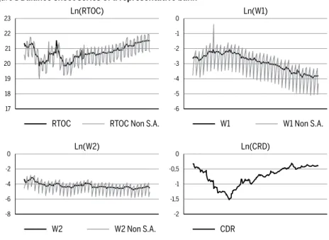
A simple graphical inspection of the series revealed that seasonality was a striking feature of some variables. This is illustrated in Figure 1 for a repre-sentative bank, whose identity is not revealed for confi dentiality reasons. The seasonal component was removed through the application of the fi l-ter CENSUS X12, provided by the United States Census Bureau, which is widely used in the treatment of seasonality in time series. The only variable that showed no seasonal movements, and consequently was not fi ltered, was the (log of) risk of the portfolio [called ln(CRD)], which was included as a control variable in the estimated models.

Table 2 Defi nition of the variables

Administrative remuneration per unit of credit granted

Remuneration for deposits

Risk from fi nancial intermediation exposure

Total revenue from credit operations

The seasonal movements are due to the occurrence of specifi c events in some periods of the year such as the payment of the 13th_{salary in} Decem-ber and other synchronized procedures in the release of accounting infor-mation. Banks have to follow accounting rules and handling accounting information might depend on the managers’ intentions, profi t distribution policies, disclosure of fi nancial results, capital structure of the institution, if it is public or privately owned, and other elements. Taken together, all previous elements contribute to introduce a typical oscillatory movement in the time series, which characterizes the seasonal component.

As illustrated in Figure 1, there is a signifi cant difference between the seasonally-adjusted series and the unadjusted ones for a representative bank.6_{In all previous studies, there was no reference to the seasonal} com-ponent of the balance sheet series. The lack of treatment for the seasonal-ity might affect the empirical results concerning the degree of competition

6 Figure 1 displays only a representative bank because of the diffi culty to plot and jointly format the series of all 62 banks. However, the series for all remaining banks showed similar patterns.

RT_OC = Income from lending operations CRD =

W 2 =

W 1 =Administrative expenses Lending operations

Borrowing expenses

(Deposits + Current and long term liabilities)

Lending operations

(11)

in the Brazilian banking sector, as it will be shown in the next section.7 Our interest is to evaluate the effects of cycle and trend components on banking concentration in Brazil. The seasonal component shall be elimi-nated from the time series because it represents a simple regular oscillation that occurs in specifi c periods of the year and that is not related to those components. It does not matter whether this seasonal component will un-der or overestimate bank competition. It only matters that the estimator is affected and, therefore, seasonality must be adequately treated. For com-parison purposes, we report estimations for time series with and without seasonal adjustment.

The Census X12 fi lter was applied to each time series individually in order to adjust for seasonality. The model was then estimated using the seasonally-adjusted series. In the presence of seasonality, the estimated coeffi cients might be biased and the explanatory power of the model might be artifi cially infl ated. The preliminary adjustment prevents sea-sonal movements from hindering the identifi cation of the relationship between the variables.

The classifi cation by Central Bank of Brazil available in the balance sheets was used to classify each bank in the sample as public (PUB), de-velopment (DES), investment (INV), foreign (EXT), and large (GRD), not necessarily mutually exclusive. The group of large institutions (GRD) was rated as the top fi ve institutions according to the highest values of total assets in the balance sheets of February, 2012. Comparing the total assets of these fi ve major banks, the smallest of them accounted for 43% of the total assets of the largest one. In addition, the sixth bank in the general classifi cation had only 14% of the total assets of the largest bank. This means that the fi fth largest bank is more than three times larger than the sixth one. Because of this disparity, they are commonly called the top fi ve Brazilian banks.

The identifi cation of each institution was possible through its unique CNPJ (Corporate Taxpayer Registry) number, which facilitates the organization and manipulation of the banks. Thus, changes in names or classifi -cations of banks during the period did not generate any diffi culty for the

(12)

organization of information. The utilization of CNPJ also allows keeping in the data set those institutions which have acquired or incorporated oth-er ones and exclude those which have been extinguished or incorporated when building a balanced panel data. It is also necessary to point out that many institutions have changed their classifi cation in the period and the correspondent qualitative variables followed those changes.

Figure 1 Balance sheet series of a representative bank

4 _Results

4.1 Unit root tests

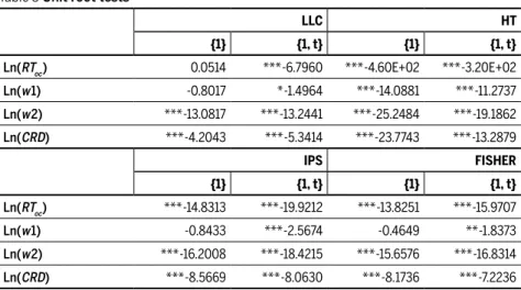
In a panel data, as in the time-series environment, there is a concern about stationarity of the variables because the presence of a unit root might lead to the estimation of a spurious regression when the residuals are not stationary. To test for the presence of unit root in the balanced panel, we applied the tests proposed by Levin-Lin-Chu (2002), called LLC, Im, Pesaran and Shin (2003), known as IPS, Fisher and Choi (2001), and Harris and Tzvalis (1999), or HT for short. We apply all these different tests in order to get some complemen-tarity in the results. For instance, LLC and HT tests are for common unit root,

0

-2

-4

-6

-8

Ln(W2)

0

-1

-1,5

-2

Ln(CRD)

-0,5

W2 W2 Non S.A. CDR

21

20

19 23

22

18

17

Ln(RTOC)

-2

-4

-5

-6

Ln(W1)

-3 0

-1

(13)

while IPS and Fisher tests deal with individual unit root; LLC and HT can be applied only for strongly balanced panel; and IPS accepts unbalanced panel but with no gaps in each individual series. The results are reported in Table 3. The variables ln(RTOC), ln(w1), and ln(w2) were seasonally-adjusted.

Table 3 Unit root tests

LLC HT

{1} {1, t} {1} {1, t}

Ln(RT_oc ) 0.0514 *** -6.7960 *** -4.60E+02 *** -3.20E+02 Ln(w 1) -0.8017 * -1.4964 *** -14.0881 *** -11.2737

Ln(w 2) *** -13.0817 *** -13.2441 *** -25.2484 *** -19.1862

Ln(CRD) *** -4.2043 *** -5.3414 *** -23.7743 *** -13.2879

IPS FISHER

{1} {1, t} {1} {1, t}

Ln(RT_oc) *** -14.8313 *** -19.9212 *** -13.8251 *** -15.9707 Ln(w 1) -0.8433 *** -2.5674 -0.4649 ** -1.8373

Ln(w 2) *** -16.2008 *** -18.4215 *** -15.6576 *** -16.8314

Ln(CRD) *** -8.5669 *** -8.0630 *** -8.1736 *** -7.2236

Notes: Lags selected by the Akaike information criteria. * Reject the null at 10% of signifi cance;

** Reject the null at 5% of signifi cance; *** Reject the null at 1% of signifi cance.

The LLC test shows different results depending on the model’s specifi ca-tions. In the equation without trend, the null of unit root was not rejected for ln(w1) and ln(RTOC ). By adding the trend, however, the unit root

hy-pothesis was rejected at the 10% signifi cance level for ln(w1) and at 1% for all other variables.

The IPS test indicated that, except for ln(w1), all variables are station-ary at the 1% signifi cance level with the inclusion of a constant. Adding a constant and a trend, all variables are stationary at the 1% signifi cance level. Similarly to LLC test, ln(w1) is stationary only in the equation that includes trend as a deterministic term.

The FISHER test practically reproduced IPS results. The only difference was that in the specifi cation with constant and trend, ln(w1) rejected H₀

(14)

ca-tions. The LLC test, despite having the same null hypothesis as the HT, required the inclusion of a linear trend to reject unit root for all variables.

The results from these four tests led to the conclusion that the panel is stationary. In general, it is suffi cient to include a constant as a deterministic term in the test equations to render stationarity for all variables. These fi ndings validate the estimation of equation (1) in log-level without incur-ring any spurious regression.

Given the stationarity of all variables, Table 4 reports the estimates for the basic model under the assumptions of fi xed effects (FE) and random effects (RE) in order to apply the Hausman test. The difference between the two estimates is very small when comparing the sum of the squared error. The Hausman test for the difference between the coeffi cients did not reject the hypothesis of identical estimates. This result indicates that the specifi c individual heterogeneity is not correlated with the regressors. Thus, the Hausman test recommends the estimation of the random effects model. As previously stated, the RE model shall be estimated by GLS to correct the variance-covariance matrix for the presence of unknown het-eroskedasticity.8

Table 4 Hausman test

FE RE S.E.

Ln(w 1) -0.3637 -0.3659 (0.0024)

Ln(w 2) -0.0790 -0.0773 (0.0013)

Ln(CRD) 0.3626 0.3601 (0.0024)

χ 2_{(3) = 2.51} _{P-value = 0.4739}

4.2 Seasonal adjustment

The results obtained from the seasonally-adjusted data indicated that the Brazilian banking sector is less competitive than what is usually found in other studies that do not perform this adjustment before estimation.9

Us-8 The results for the basic model estimated under FE and RE reported in Table 4 indicates that there is no signifi cant difference between the coeffi cients estimated from these two alternative specifi cations. Thus, there is also no signifi cant difference in the H-statistics esti-mated from each one of those models. Specifi cally, the H-statistics were -0.4427 and -0.4432 for the FE and RE models, respectively.

(15)

ing non-seasonally-adjusted data, all estimates of the H-statistics were sig-nifi cantly larger and always positive (H > 0), according to other studies on the Brazilian economy. This fi nding suggests that a preliminary treatment of the banking time series is crucial for the assessment of the level of com-petition in the sector. If seasonality is not removed from the database, all bank profi les would be erroneously classifi ed as operating in monopolistic competition. This result is in accordance with Belaisch (2003), Lucinda (2010) and Araujo and Jorge Neto (2007), who do not mention any treat-ment for seasonal effects in their database.

Table 5 presents, side by side, the estimates from the seasonally-ad-justed and non-seasonally-adseasonally-ad-justed series. Comparing the results, several coeffi cients show signifi cant changes between the two models. In addi-tion, the explanatory power of the regression is higher in the seasonally-adjusted model, as illustrated by the R² of 0.3043 against 0.2563 in the non-seasonally-adjusted model.

Table 5 Effects of seasonality in the estimated models

Variable Seasonally-adjusted Non-seasonally-adjusted

Ln(w 1) *** -0.4070

(0.0316)

-0.0006 (0.0282)

Ln(w 2) *** -0.1025

(0.0264)

*** 0.1061 (0.0260)

gw 1m *** -0.6115

(0.1046)

*** -0.6156 (0.1005)

gw 2_m *** 0.3143

(0.1576)

*** 0.7892 (0.1211)

pw 1_m 0.0606

(0.0999)

0.0958 (0.0908)

pw 2_m ** 0.2187

(0.1127)

** 0.2204 (0.0975)

ew 1_m ** -0.1247

(0.0709)

-0.0894 (0.0647)

dummies in the regression or if the variable is fi rst seasonally adjusted (by the same dummy variable method), and then the regression is estimated. As the estimation of a regression with seasonal dummies is part of the procedure applied by the Census X12, the results obtained with the inclusion of dummies variables in a regression with unadjusted time series are very similar to the ones reported in Table 5.

(16)

ew 2_m *** 0.2310

(0.0618)

*** 0.1664 (0.0597)

iw 1_m *** 0.7570

(0.0869)

*** 0.5495 (0.0881)

iw 2_m 0.2505

(0.1595)

-0.1397 (0.1264)

dw 1_m 0.2223

(0.1895)

*** 0.3695 (0.1164)

dw 2_m -0.0393

(0.0470)

*** -0.2420 (0.0475)

Ln(CRD) *** 0.3571

(0.0341)

*** 0.6229 (0.0343)

grd_n *** 3.7208

(0.9158)

*** 5.7003 (0.7469)

pub_n *** 2.6819

(0.7127)

*** 2.7597 (0.6048)

ext_n *** 0.8616

(0.2868)

*** 0.8025 (0.2403)

inv_n *** 2.9394

(0.5761)

* 0.7668 (0.4054)

des_n 1.0808

(1.3298)

1.4851 (1.1219)

_cons *** 13.8941

(0.2264)

*** 16.0372 (0.2116)

R² 0.3049 0.2544

N 13144 13144

Notes: subscript m represents the multiplicative dummy for the group of banks: large (g), public (p), foreign (e), investment (i), and development (d). Subscript n stands for level dummies for large banks (grd), public banks (pub), foreign banks (ext), investment banks (inv), and development banks (des). ***, **, and * - statistically signifi cant at the 1, 5 and 10% signifi cance levels, respectively. N is the num-ber of observations. Robust standard errors are in parenthesis.

(17)

among the control groups, with some increasing and others decreasing the estimated coeffi cients. As the computation of the H-statistics requires a joint analysis of these coeffi cients, we have to observe the changes in the H-statistics in order to identify the effects of the seasonal adjustment for the market structure for the Brazilian banking sector.

The behavior of the H-statistics in the non-seasonally-adjusted data is quite different from the seasonally-adjusted one, as reported in Table 6. In the fi rst case, all control groups showed positive H-statistics (H > 0), result-ing in market structures of imperfect or monopolistic competition. Only for the development banks, did the test not reject the non-competitive hypothesis (H ≤ 0). For the seasonally-adjusted data, however, the result is the opposite. The group of investment banks presented positive H-sta-tistics, which is consistent with imperfect competition. All other groups displayed negative H-statistics, which are not compatible with competi-tive market structures. These results reveal a tendency to overestimate the H-statistics when there is seasonality in the data which is not treated prior to the estimation.

Table 6 Seasonal adjustment and H-statistics

Banks Seasonally-adjusted Non-seasonally-adjusted

H_grd -0.8066***

(0.1696)

0.2791*** (0.0870)

H_pub -0.2302*

(0.1293)

0.4218*** (0.0669)

H_ext -0.4033***

(0.0793)

0.1826*** (0.0592)

H_inv 0.4979***

(0.1386)

0.5153*** (0.0889)

H_des -0.3265*

(0.1942)

0.2330** (0.1131)

H_geral -0.5095***

(0.0337)

0.1055*** (0.0235)

Notes: *** - P-value < 0.01; ** - P-value < 0.05; * - P-value < 0.10 for the Wald test.

(18)

variables (not reported in his paper), but argued that the estimates of the H-statistics were even greater than when scale variables were included. Finally, it is noteworthy that the similarity of the non-seasonally-adjusted results from Table 5 with those of Tabak, Gomes, and Medeiros Junior (2015) reinforces the fact that omitting such treatment might bias the as-sessment of the correct market structure for the Brazilian banking sector.

4.3 Scale variables

The inclusion of scale variables in the estimation of banking competition is a recurring theme in the literature. Their effects in a seasonally-adjusted environment, however, are not yet well explored. The log of total depos-its10_{was added as an explanatory variable in the models presented in Table} 5 and the new results are reported in Table 7. This represents a scale vari-able also used in other studies as control for the size of banks.11_{The effects} appear in the different values of the estimated coeffi cients by the adjusted and unadjusted models for seasonality.

Comparing the results from Tables 7 and 5, one can see that most coef-fi cients, for both models, suffered changes, which refl ects a relationship between price of inputs and revenue. According to Bikker, Shaffer and Spierdijk (2012), the estimated regression would no longer represent the reduced-form revenue but, instead, the effect of the price of the good as the coeffi cient of the scale variable approaches the unit. In Table 7, this co-effi cient is between 0.43 and 0.51, indicating an intermediate case. The ex-planatory power of the models, with R2_{coeffi cients near 50%, is relatively} high. Considering the basic model, without dummy variables, the value of R2_{was almost the same, suggesting that the inclusion of Total Deposits} as an explanatory variable might reduce the ability of the dummies to add information to the estimated model.

The effects of including scale variables might be observed by calcu-lating the H-statistics, as reported in Table 8, which also replicates the values from Table 6. Comparing the H-statistics with and without scale variable, the estimated coeffi cients are quite different. The H-statistics

(19)

for both models, with and without seasonal adjustment, are smaller in absolute value. Only development banks showed an H-statistics slightly larger in absolute value. In general, the increase is greater for the season-ally-adjusted model.

The scale variable might bias the estimates and affect the analysis of competition for public banks, which display an H-statistics compatible with competitive markets. Investment banks do not reject the hypothesis of perfect competition. The changes in the H-statistics also affect the rank-ing of market power for each group of institutions.

Table 7 Estimations with a scale variable

Ln(w 1) *** -0.1335

(0.0321)

*** 0.2141 (0.0282)

Ln(w 2) *** -0.1788

(0.0258)

-0.0400 (0.0255)

gw 1 _m *** -0.2817

(0.1046)

*** -0.2861 (0.0996)

gw 2 _m ** 0.3994

(0.1571)

*** 0.5354 (0.1200)

pw 1 _m -0.0014

(0.0977)

-0.0617 (0.0888)

pw 2 m *** 0.4496

(0.1123)

*** 0.4185 (0.0958)

ew 1 _m -0.0750

(0.0691)

-0.0679 (0.0624)

ew 2 _m *** 0.2652

(0.0600)

*** 0.2169 (0.0574)

iw 1 _m *** 0.5401

(0.0827)

*** 0.3683 (0.0834)

iw 2 _m *** 0.4690

(0.1575)

0.0400 (0.1229)

dw 1 _m -0.0368

(0.1469)

** 0.2085 (0.1046)

dw 2 _m *** -0.1490

(0.0463)

*** -0.3042 (0.0465)

(20)

Ln(CRD) *** 0.6596

(0.0351)

*** 0.9054 (0.0344)

grd _n *** 3.0874

(0.6786)

*** 3.3105 (0.4293)

pub _n *** 2.6729

(0.5041)

*** 2.2203 (0.3384)

ext _n ** 0.7059

(0.2835)

** 0.5489 (0.2360)

inv _n *** 3.4081

(0.5606)

*** 1.3014 (0.3924)

des _n -1.0710

(0.7768)

-0.2705 (0.5977)

Deps *** 0.4300

(0.0168)

*** 0.5122 (0.0167)

_cons *** 8.6607

(0.2459)

*** 9.2109 (0.2469)

R² 0.521 0.4984

N 13144 13144

Banks in general, in the seasonally unadjusted model of Table 8 with scale variable, have a lower H-statistics than that obtained by Belaisch (2003), Araújo and Jorge Neto (2007) and Lucinda (2010), but higher than Tabak, Gomes, and Medeiros Junior (2015). For the control groups, the model without seasonal adjustment and with scale variables presented 0 < H < 1. This result indicates the existence of monopolistic competition in the banking sector, as do most of the empirical works in the literature for the Brazilian economy.

One can also observe that the inclusion of scale variable in the esti-mated regressions overestimates the H-statistics for both commercial and investment banks. However, it underestimates the H-statistics for devel-opment banks, regardless of the seasonal adjustment of the data.

(21)

Table 8 Estimated values for the H-statistics

Bank type With scale variable Without scale variable

Seasonally--adjusted Non-seasonally--adjusted Seasonally--adjusted Non-seasonally--adjusted H_grd -0.1945 (0.1702) *** 0.4235 (0.0862) *** -0.8066 (0.1696) *** 0.2791 (0.0870) H_pub 0.1359 (0.1282) *** 0.5309 (0.0663) * -0.2302 (0.1293) *** 0.4218 (0.0669) H_ext -0.1220 (0.0793) *** 0.3232 (0.0586) *** -0.4033 (0.0793) *** 0.1826 (0.0592)

H_inv *** 0.6969

(0.1368) *** 0.5825 (0.0877) *** 0.4979 (0.1386) *** 0.5153 (0.0889)

H_des *** -0.4981

(0.1507) 0.0784 (0.1019) * -0.3265 (0.1942) ** 0.2330 (0.1131)

H_geral *** -0.3123 (0.0328) *** 0.1741 (0.0230) *** -0.5095 (0.0337) *** 0.1055 (0.0235)

Notes: *** - P-value < 0.01; ** - P-value < 0.05; * - P-value < 0.10 for the Wald test.

In addition to the seasonal adjustment and inclusion of a scale variable in the regressions, it is necessary to emphasize the change in computation of the administrative remuneration per unit of credit (w1). In general, this variable is separated into average earnings of the workforce and unit price of other costs, such as physical capital, administrative expenses or non-operating expenses. Here, this variable is defi ned in terms of units of its output, which is credit granted and not total assets. With w1 expressed per unit of credit granted and separating the panel on sequential cross sections, the result H < 0 was maintained in all scenarios: seasonally-adjusted, non-seasonally-adjusted, with or without scaling variables.

4.4 Market structure of the banking sector

(22)

H-statistics. This happens because these three groups are not mutually exclusive, having banks that enter in more than one classifi cation. The complete regression shall be used in the analysis because it controls for the profi le of each kind of institution.

Table 9 Estimations for the complete model and specifi c groups

Complete Big Public Foreign

Invest-ment

Develop-ment

Basic

Ln(w 1) *** -0.4070 (0.0316) *** -0.3313 (0.0287) *** -0.3581 (0.0288) *** -0.3511 (0.0292) *** -0.4342 (0.0285) *** -0.3788 (0.0287) *** -0.3659 (0.0282)

Ln(w 2) *** -0.1025 (0.0264) *** -0.0868 (0.0200) *** -0.0865 (0.0202) *** -0.0984 (0.0214) *** -0.0783 (0.0199) ** -0.0533 (0.0231) *** -0.0773 (0.0199)

gw 1 _m *** -0.6115 (0.1046)

*** -0.6660 (0.0983)

- - - -

-gw 2 _m ** 0.3143 (0.1576)

*** 0.3983 (0.1511)

- - - -

-pw 1 _m 0.0606 (0.0999)

- *** -0.2264 - - -

-pw 2 _m ** 0.2187 (0.1127)

- *** 0.2963 - - -

-ew 1 _m ** -0.1247 (0.0709)

- - *** -0.1730 - -

-ew 2 m 0.2310

(0.0618)

- - *** 0.2228 - -

-iw 1 _m *** 0.7570 (0.0869)

- - - *** 0.7930 -

-iw 2 _m 0.2505 (0.1595)

- - - 0.2172 -

-dw 1 _m 0.2223 (0.1895)

- - - - 0.2651

-dw 2 _m -0.0393 (0.0470)

- - - - -0.0863

-Ln(CRD) *** 0.3571 (0.0341) *** 0.3527 (0.0340) *** 0.3497 (0.0342) *** 0.3560 (0.0341) *** 0.3737 (0.0340) *** 0.3561 (0.0341) *** 0.3601 (0.0341)

grd _n *** 3.7208 (0.9158)

*** 4.3571 (0.9486)

- - - -

(23)

Complete Big Public Foreign Invest-ment

Develop-ment

Basic

pub n 2.6819

(0.7127)

- *** 3.0682 (0.8103)

- - -

-ext _n 0.8616 (0.2868)

- - *** 0.7384 (0.2852)

- -

-inv n 2.9394

(0.5761)

- - - *** 2.9052 (0.5753)

-

-des _n 1.0808 (1.3298)

- - - - 0.5894

(1.6911)

-_cons 13.8941 (0.2264)

*** 14.3544 (0.2304)

*** 14.3322 (0.2633)

*** 14.5982 (0.2691)

*** 14.4909 (0.2749)

*** 14.7199 (0.2768)

*** 14.6621 (0.2736)

R² 0.3049 0.2722 0.1447 0.0413 0.0548 0.0439 0.0486

N 13144 13144 13144 13144 13144 13144 13144

Assessing the H-statistics for the complete regression in Table 10, only investment banks showed a positive coeffi cient and were statistically dif-ferent from both 0 and 1. This is representative of the monopolistic com-petition case. This fi nding is in line with the characteristics of these institu-tions, because investment banks have a smaller base of clients compared to commercial banks. But these special clients get high loan volumes and are charged lower interest rates when compared to clients of commer-cial banks. Investment banks do not accept deposits and have to appeal to banking credit market in order to fi nance loans. Basically, the reduced number of exclusive clients and the large volume of each credit operation encourage the competition among investment banks.

(24)

Table 10 H-statistics for specifi c bank groups

Complete Big Public Foreign

Invest-ment Develop-ment Basic H_grd -0.8066 (0.1696) -0.6858 (0.1603) -H_pub -0.2302 (0.1293) --0.3746 (0.1221) -H_ext -0.4033 (0.0793) --0.3997 (0.0800) -H_inv 0.4979 (0.1386) -0.4976 (0.1389) -H_des -0.3265 (0.1942) --0.2533 (0.1997) -H_geral -0.5095 (0.0337) -0.4181 (0.0299) -0.4445 (0.0301) -0.4495 (0.0307) -0.5126 (0.0297) -0.4321 (0.0305) -0.4432 (0.0294)

Note: The fi rst column corresponds to the model with all dummies. The last column corresponds to the model without dummies. The remaining columns consider only one group at a time. Reported statistics are for the Wald test.

Compared to other studies for the Brazilian economy that apply the Panzar-Rosse method, Table 10 reports different results. Lucinda (2010) is methodologically closest to our approach but he fi nds an H-statistics of 0.8, much higher than the value of -0.51 reported in Table 10. Tabak, Gomes, and Medeiros Jr. (2015), despite fi nding an average value of 0.116 for the H-statistics, which is lower than Lucinda (2010), is still much high-er than the value obtained hhigh-ere. Belaisch (2003) fi nds results even more discrepant, with the H-statistics so high that in some cases it is not pos-sible to reject the hypothesis of perfect competition. At the aggregate state level, Sanches et al. (2009) claim that the degree of banking competition is high, but not perfectly competitive, across the major Brazilian states.

(25)

multi-product structure of Brazilian banks might lead to underestimation of the market power of these banks.

5 _{Concluding remarks}

The objective of this paper was to access the level of competition in the Brazilian banking market by applying the Panzar-Rosse model to a bal-anced panel data with 62 fi nancial institutions from July 1994 to February 2012. Compared to other studies that indicated a market structure com-patible with monopolistic competition, the results obtained here highlight the importance of incorporating in the analysis the seasonal adjustment of the data, the criticism by Bikker, Spierdijk, and Shaffer (2012) on the inclu-sion of scale variables and the normalization of administrative expenses per unit of credit granted.

The choice of the basic model followed Bikker, Spierdijk, and Shaffer (2012), who suggested the exclusion of any scale variable from the regres-sion and any scale control among the variables. The sensitivity analysis about the effects of scale variables in the regression illustrates that the criticism is valid for the Brazilian case. In general, the model with a scale variable overestimates the H-statistics, erroneously indicating the exis-tence of some structure of competition in the banking sector.

Equally important to the accuracy of the results was the preliminary treatment of the seasonal effect observed in the fi nancial variables. The presence of seasonality affected the estimated coeffi cients and the H-sta-tistics. Studies that ignore the seasonal effect tend to incorrectly conclude that there are competitive structures in the Brazilian banking market, when there is considerable market power for the banks in general and other specifi c groups.

(26)

Belaisch (2003), Araujo and Jorge Neto (2007), Lucinda (2010), and Tabak, Gomes, and Medeiros Jr. (2015) might exhibit the seasonal bias in addition to problems associated with the use of scale variables.

Our fi ndings reveal that, in general, Brazilian banks are not competi-tive. The exceptions are investment banks, which have an H-statistics compatible with a monopolistic competition market structure. The fi ve biggest banks are not competitive and their market power is consider-ably higher than that of the other institutions. This might help to explain the high profi tability and high interest rates practiced by banks in the Brazilian economy.

Public banks have lower market power than banks in general. However, these banks do not act as if they were in perfect competition. This is due to political interference in management decisions that public banks are frequently subject to, distancing them from the behavior of private institu-tions that seek profi t maximization.

These fi ndings differ from those of other studies for the Brazilian economy, including Belaish (2003), Araujo and Jorge Neto (2007), Lucinda (2010), and Tabak, Gomes, and Medeiros Jr (2015). We provided empirical evidence that the Brazilian banking sector does not operate under com-petition, contrary to the fi ndings provided by those authors. Recently, Barbosa et al. (2015) also found evidence of high market power in the banking sector after taking into account the multi-product structure of the Brazilian banks. For further research, one should evaluate the effi ciency of distinct seasonal adjustment methods applied to fi nancial series, compute the Lerner Index, and extend the discussion on how the normalization of input prices might generate alternative ways of working with the Panzar-Rosse model.

References

ARAÚJO, L. A. D. D.; JORGE NETO, P. D. M.; PONCE, D. A. S. Competição e Concentração entre os Bancos Brasileiros. Revista Economia, v.7, n.3, p.561–586, 2006.

ARAÚJO, L. A. D. D.; JORGE NETO, P. D. M. Risco e competição bancária no Brasil. Revista Brasileira de Economia, v. 61, n. 2, p. 175-200, 2007.

BARBOSA, K.; ROCHA, B. P.; SALAZAR, F. Assessing competition in the banking industry: A multi-product approach. Journal of Banking and Finance, v. 50, p. 340-62, 2015.

(27)

BIKKER, J. A.; HAAF, K. Competition, concentration and their relationship: An empirical analysis of the banking industry. Journal of Banking and Finance, n. 26, p. 2191-2214, 2002. BIKKER, J. A.; SHAFFER, S.; SPIERDIJK, L. Assessing competition with the Panzar-Rosse

model: The role of scale, costs, and equilibrium. The Review of Economics and Statistics, MIT Press, vol. 94(4), p. 1025-1044, 2012.

BRESNAHAN, T. F. The oligopoly solution is identifi ed. Economics Letters, n. 10, p. 87-92, 1982. CHOI, I. Unit root tests for panel data. Journal of International Money and Finance, n. 20,

p. 249-272, 2001.

HARRIS, R. D. F.; TZAVALIS., E. Inference for unit roots in dynamic panels where the time dimension is fi xed. Journal of Econometrics, n. 91, p. 201–226, 1999.

IM, K. S.; PESARAN, M. H.; SHIN., Y. Testing for unit roots in heterogeneous panels. Journal of Econometrics, v. 115, p. 53–74, 2003.

LAU, L. J. On identifying the degree of competitiveness from industry price and output data. Economics Letters, n. 10, p. 93-99, 1982.

LEVIN, A.; LIN, C. F.; CHU, C.-S. J. Unit root tests in panel data: asymptotic and fi nite-sample properties. Journal of Econometrics, v. 108, n. 1, p. 1-24, 2002.

LUCINDA, C. R. Competition in the Brazilian loan market: An empirical analysis. Estudos Econômicos, São Paulo, v. 40, p. 831-858, 2010.

NAKANE, M. I. A test of competition in Brazilian banking. Estudos Econômicos, n. 32, p. 203-224, 2002.

PANZAR, J. N.; ROSSE, J. Testing for monopoly equilibrium. Journal of Industrial Economics, n. 35, p. 443-456, 1987.

SANCHES, F. M.; ROCHA, B. P.; SILVA, J. C. Estimating a Theoretical Model of State Banking Competition Using a Dynamic Panel: The Brazilian Case. Revista Brasileira de Economia, v. 63, p. 23-34, 2009.

SHAFFER, S. The Rosse Panzar statistic and the Lerner index in the short run. Economics Letters, n. 11, p. 175-178, 1983.

TABAK, B. M.; GOMES, G. M. R.; MEDEIROS JÚNIOR, M. D. S. The impact of market pow-er at bank level in risk-taking: The Brazilian case. Intpow-ernational Review of Financial Analysis, v. 40, p. 154–165, 2015.

About the authors

José Angelo Divino - jangelo@pos.ucb.br

Universidade Católica de Brasília. Brasília, Distrito Federal.

Renan Said Silva - renansaiducb@hotmail.com

Universidade Católica de Brasília. Brasília, Distrito Federal.

The authors would like to thank participants in the XLI Meeting of the Brazilian Economic Association (ANPEC) for the helpful comments and suggestions and CNPq for fi nancial support. All remaining errors are the authors’ sole responsibility.

About the article