INSTITUTO DE TECNOLOGIA
PROGRAMA DE PÓS-GRADUAÇÃO EM ENGENHARIA ELÉTRICA
A Comparison between RS+TCM and LDPC
FEC schemes for the G.fast standard
Marcos Yuichi Takeda
DM 04/2016
UFPA / ITEC / PPGEE
Campus Universitário do Guamá Belém - Pará - Brasil
PROGRAMA DE PÓS-GRADUAÇÃO EM ENGENHARIA ELÉTRICA
A Comparison between RS+TCM and LDPC
FEC schemes for the G.fast standard
Autor: Marcos Yuichi Takeda
Orientador: Aldebaro Barreto da Rocha Klautau Júnior
Dissertação submetida à Banca Examinadora do
Programa de Pós-Graduação em Engenharia Elétrica da Universidade Federal do Pará para obtenção do
Grau de Mestre em Engenharia Elétrica. Área de concentração: Telecomunicações.
UFPA / ITEC / PPGEE Campus Universitário do Guamá
INSTITUTO DE TECNOLOGIA
PROGRAMA DE PÓS-GRADUAÇÃO EM ENGENHARIA ELÉTRICA
A Comparison between RS+TCM and LDPC FEC schemes for the
G.fast standard
AUTOR(A): MARCOS YUICHI TAKEDA
DISSERTAÇÃO DE MESTRADO SUBMETIDA À AVALIAÇÃO DA BANCA
EX-AMINADORA APROVADA PELO COLEGIADO DO PROGRAMA DE PÓS-GRADUAÇÃO EM ENGENHARIA ELÉTRICA, DA UNIVERSIDADE
FED-ERAL DO PARÁ E JULGADA ADEQUADA PARA A OBTENÇÃO DO GRAU DE MESTRE EM ENGENHARIA ELÉTRICA NA ÁREA DE
TELECOMUNI-CAÇÕES.
Prof. Dr. Aldebaro Barreto da Rocha Klautau Júnior (Orientador - UFPA / ITEC)
Prof. Dr. Evaldo Gonçalves Pelaes (Membro - UFPA / PPGEE)
Profa. Dra. Valquíria Gusmão Macedo
I would like to thank every colleague, friend, professor that I had contact at this 3 years of master degree program. The year of 2015 was a life changer year for me, as I was
diagnosed with cancer. This result in almost a year of delay due to cancer treatment, namely chemotherapy and radiotherapy. Fortunately, the treatment worked well and now I could
finally write this disseratation thesis.
Thus I want to truly thank everyone who gave me support during the heavy cancer
treatment. My family, Kazuo, Maria and Akira Takeda, in first place, and friends from LaPS, and in special my advisor Prof. Aldebaro Klautau, which was very comprehensive, my
former coadvisor Fernanda Smith, which took my place at a paper presentation when I was at treatment. Special thanks to Pedro Batista, Bruno Haick, Francisco Muller, Ana Carolina,
Silvia Lins, Igor Almeida, Leonardo Ramalho, Joary Fortuna, Igor Freire, Kelly Souza, and many others from LaPS.
Also, I would want to thank friends outside UFPA and LaPS, that were invaluable during my treatment.
The need for increasing internet connection speeds motivated the creation of a new standard, G.fast, for digital subscriber lines (DSL), in order to provide fiber-like performance using
short twisted pair copper wires. This dissertation focuses in the two former candidate codes for the forward error correction (FEC) scheme, namely Reed-Solomon (RS) with trellis-coded
modulation (TCM), from previous DSL standards, and low density parity check (LDPC) codes, from the G.hn standard for home networking. The main objective is to compare both
schemes, in order to evaluate which of them performs better, considering metrics such as error correction performance and computational cost. Even though the selected code for G.fast was
A necessidade de velocidades de conexão a internet cada vez maiores motivou a criação de
um novo padrão, G.fast, para DSL (linha digital do assinante), de modo a prover performance semelhante a fibra usando par trançado de fios de cobre. Esta dissertação foca em dois
prévios candidatos a esquemas de correção de erro, sendo eles codigos Reed-Solomon com modulaçao codificada em treliça (TCM), de padrões DSL anteriores, e códigos de verificação
de paridade de baixa densidade (LDPC), do padrão G.hn para redes residenciais. O objetivo principal é comparar os dois esquemas, de modo a avaliar qual deles tem melhor performance,
considerando métricas como poder de correção de erro e custo computacional. Embora o código selecionado para o G.fast já tenha sido RS+TCM, acredita-se que esta decisão foi
List of Figures iv
List of Tables vi
List of Symbols vii
Introduction 1
1 Fundamentals of channel coding 4
1.1 Channel Coding . . . 4
1.1.1 Block codes . . . 5
1.1.2 Convolutional codes . . . 6
1.2 Reed-Solomon codes . . . 9
1.2.1 Finite fields . . . 11
1.2.2 Encoding . . . 13
1.2.3 Decoding . . . 14
1.3 Trellis-coded modulation . . . 15
1.3.1 Encoding/Mapping . . . 16
1.3.2 Decoding/Demapping . . . 16
1.4 Low-Density Parity-Check codes . . . 17
1.4.1 Encoding . . . 17
1.4.2 Decoding . . . 18
2 Standards Overview 19 2.1 G.fast forward error correction . . . 19
2.1.1 Reed-Solomon . . . 19
2.1.1.4 Unshortening . . . 24
2.1.2 Interleaving . . . 24
2.1.2.1 Deinterleaving . . . 26
2.1.3 Trellis-coded modulation . . . 26
2.1.3.1 Bit extraction . . . 26
2.1.3.2 Encoding . . . 27
2.1.3.3 QAM modulation . . . 28
2.1.3.4 QAM demodulation . . . 29
2.1.3.5 Decoding . . . 31
2.2 G.hn forward error correction . . . 35
2.2.1 LDPC . . . 36
2.2.1.1 Encoding . . . 37
2.2.1.2 Puncturing . . . 39
2.2.1.3 Constellation Mapper . . . 39
2.2.1.4 Demapper . . . 41
2.2.1.5 Depuncturing . . . 41
2.2.1.6 Decoding . . . 42
3 Results 46 3.1 Error correction performance . . . 46
3.1.1 Metrics . . . 46
3.1.2 Simulation . . . 48
3.1.3 Results . . . 50
3.2 Complexity . . . 52
3.2.1 Metrics . . . 52
3.2.2 Results . . . 53
3.2.2.1 G.fast complexity . . . 53
3.2.2.2 G.hn complexity . . . 56
3.2.2.3 Remarks . . . 58
4.1 Future works . . . 60
Bibliography 61
1.1 Systematic codeword generation by a block code. . . 6
1.2 Representation of a convolutional code as parities on a sliding window. . . 7
1.3 State diagram. . . 8
1.4 Trellis diagram. . . 8
2.1 Reed-Solomon Encoding Filter. . . 21
2.2 Decoder blocks. . . 21
2.3 Shortening process. . . 23
2.4 Each step of Reed-Solomon encoding. . . 23
2.5 Each step of Reed-Solomon decoding. . . 24
2.6 Interleaver matrix and the values for each index. . . 25
2.7 Finite state machine form of the trellis code. . . 27
2.8 Relation ofuˆwith vˆand wˆ. . . 28
2.9 Modulation algorithm. . . 29
2.10 2-dimensional cosets in a QAM constellation. . . 29
2.11 2D and 4D distance metrics. . . 31
2.12 Relation between 2D and 4D cosets, from G.fast standard. . . 32
2.13 Trellis diagram from G.fast. . . 33
2.14 Viterbi algorith diagram example. . . 36
2.15 Encoding process. . . 40
2.16 Depuncturing process. . . 42
2.17 Check-node processing. . . 43
2.18 Bit-node processing. . . 43
2.19 Initialization. . . 44
2.20 A posteriori LLR calculation. . . 44
3.2 RS+TCM vs LDPC on 1024-QAM. . . 51 3.3 Comparison to Shannon capacity. . . 52
1.1 Addition and multiplication tables. . . 12
1.2 Three different views of GF(4). . . 13
1.3 Addition and multiplication tables for GF(4). . . 13
2.1 Distance by 4-D cosets. . . 35
2.2 Summary of G.hn parity check matrices . . . 38
2.3 Dimensions of sub-blocks (in compact form). . . 38
2.4 Puncturing Patterns. . . 41
ACS Add-compare-select
API Application Programming Interface
AWGN Additive White Gaussian Noise
BCH Bose-Chaudhuri-Hocquenghem
BER Bit error rate
BLER Block error rate
BMU Branch metric unit
CD Compact disc
DMT Discrete multitone
DSL Digital subscriber line
DVB Digital video broadcasting
GF Galois Field
LDPC Low-density parity-check
LLR Log-likelihood ratio
LSB Least significant bit
MSB Most significant bit
OFDM Orthogonal frequency division multiplexing
QAM Quadrature amplitude modulation
QC-LDPC-BC Quasi-cylic low-density parity-check block code
RS Reed-Solomon
SNR Signal-to-noise ratio
TBU Traceback unit
TCM Trellis-coded modulatin
VDSL2 Very-high-bit-rate digital subscriber line 2
XOR Exclusive or
In light of the new G.fast standard for fiber-like speeds over twisted pair copper wires, there was a discussion at which forward error correction scheme would be used in the physical layer. The two main candidate schemes were Reed-Solomon codes with trellis-coded modu-lation, repeated from previous DSL standards like VDSL2, and LDPC codes, from the G.hn standard for home networks.
G.fast
The G.fast [1] standard was devised to provide up to 1 Gbps aggregated (uplink and downlink) rate over short twister pair copper wires. The motivation is to provide cabled infrastructure at a lower cost than using optical fiber. A deployment scenario example is a building, where the fiber reaches the base level and the network is further spread up using copper.
Technology
G.fast uses discrete multitone modulation (DMT), which can be viewed as a special case of orthogonal frequency division multiplexing (OFDM). DMT divides the channel into smaller non-overlapping sub-channels, transmitting a variable amount of bits depending on the conditions of each sub-channel. G.fast uses QAM in each sub-channel, with each sub-carrier using up to 4096-QAM (12 bits).
The use of DMT incur in a bitloading algorithm with channel estimation. This calcu-lates precisely how many bits can be transmitted at each sub-channel, resulting in a efficient adaptation to the channel. As seen later, the use of a bitloading table plays a important role on using trellis-coded modulation on DMT systems.
Reed-Solomon code [2] is a classical code with its main characteristic of having absolute control over its error correction properties. Also, they are used in a variety of applications as CDs, Blu-rays, barcodes, QR codes and secret sharing schemes as well. Basically, a Reed-Solomon code can correct half the number of the redundancy it inserts at a system.
Trellis-coded modulation [3] is also a classical scheme developed first for old telephone modems. Trellis-coded modulation introduction was revolutionary at the time, as it provided a way to jump from rates of 14 kbps to 33 kbps. It improved systems by increasing the number of bits per symbol instead of using more bandwidth.
LDPC
In the other hand, LDPC codes were discovered at 1963 [4], but remained forgotten for more than 30 years, because at the time the computational cost was not practical. With its rediscovery 30 years later, it gained rapid popularity as it managed to surpass the recent discovered Turbo codes. LDPC and Turbo codes belong to a class of codes called capacity ap-proaching. In fact, LDPC codes, when used with very long codeword sizes, could achieve error correction curves within 0.0045dB in Eb/N0 of the Shannon limit on AWGN channels, which
is the theoretical limit of reliable transmission [5]. LDPC works by using long codewords and sparse parity check matrices. Its design can be pseudo-random, and its exact error correction performance is difficult to calculate. Generally, we measure the average behaviour of a LDPC code, as opposed to Reed-Solomon code, where we do not even need to measure, as the error correction performance is fixed at the design. Also, LDPC decoders use probabilities instead of bits, avoiding early loss of information caused by the hard decisions caused by demodulation.
State of art
Comparison motivation
In the end, the scheme of Reed-Solomon with trellis-coded modulation was chosen for the G.fast 100 MHz profile. Although this decision was already made, it is believed that it was biased to remain unchanged, and thus favoring existing implementations. At AWGN channel tests, the error correcting performance of Reed-Solomon with trellis-coded modulation was lower than that of LDPC. One may argue with computational cost and complexity, but this remains as a very difficult question, as specialized hardware exist for both schemes.
Outline
Fundamentals of channel coding
This chapter contains a brief review of the fundamentals of channel coding, with em-phasis on the codes used on this works, namely Reed-Solomon codes, trellis-coded modulation and LDPC. This work will not assess all the details of coding theory, as there are a number of references which contain them [7–9].
1.1
Channel Coding
Channel coding is a way to improve efficiency in telecommunications systems. We can only get close to the so-called Shannon’s channel capacity by using it. The channel can be anything: a cable, air, vacuum or even a media CD or hard drive. When information is sent/written to, or received/read from a channel, noise may corrupt data. The main concept of channel coding is to add controlled redundancy data to the information data in order to protect this information from such noise. Noise is anything undesirable, and out of our control that corrupts data such as thermal noise on cables or scratches on the CD surface.
A code can be defined as a set of codewords. A codeword is a representation of an array of symbols. A symbol can be one or more bit. When we use a bit as a symbol the code is said binary. The main motivation behind using a set of codewords to represent data is that we can expand the “space” between valid sequences. An analogy can be made with digital modulation: When dealing with modulation, the values are continuous, so to “open space” we just scale the constellation by a factor greater than1, increasing the distance between points. In a code, the values are discrete and finite, so we need to map these values to a “bigger space” in order to make room for possible errors that may occur. The mapping procedure is called encoding, and the resulting values on which the original are mapped into form the code. The decoding
procedure can be also seen as an analogy to modulation: the decoder receives a value, which is not necessarily valid, so we need to find the “nearest” valid value to the received value. The process of finding this nearest is called decoding.
The main objective of channel coding in telecommunications is to achieve transmission rates near the channel capacity. The channel capacity [10] for AWGNis calculated by
C = log2(1 +SNR), (1.1) where C is the channel capacity in bits per channel use. Shannon proved in the noisy-channel
coding theorem that we can get arbitrarily close to C using an appropriate code. The main
problem is finding such a code. Also, for practical reasons, it is preferred that this code has manageable computational complexity for encoding and decoding. The word “redundancy” may sound as something that is not entirely necessary, but in channel coding it is the key to achieve optimal rates of transmissions in noisy channels.
Channel coding may be divided in two categories: Block codes and Convolutional codes.
1.1.1
Block codes
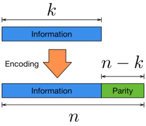
Block codes use fixed lengths for both data and redundancy. A Hamming(7,4) code is an example of a block code. It takes 4 information bits and creates more 3 bits of redundancy, comprising a codeword with 7 bits. Note that the new codeword may not resemble the original information at first glance, as we can further classify a code which maintain the original information in the codeword as systematic, and a code which does not as non-systematic. But this does not mean that non-systematic codes are not usable, as the original information can be recovered by using proper decoding algorithms. Nevertheless, the codes in this work are all from telecommunications standards, which use mostly systematic codes, justified by the fact that if a codeword is not corrupted, then we can just remove the redundancy and retrieve information more easily.
A linear block code is defined by ak×nmatrixG, called generator matrix, or(n−k)×n
matrix H, called parity-check matrix. We need just one of them, as given one, it is possible to calculate the other. The rows of G define a base of a k-dimensional vectorial subspace. Any vector in this subspace is called a codeword. The rows of H define the null space of the rows
of G, such thatGHT = 0, meaning that any codewordˆcmultiplied withHT results in0. The
code rate of a linear block code is Rblock =k/n.
Information
Information Parity Encoding
k
n
n
−
k
Figure 1.1: Systematic codeword generation by a block code.
this case the left side of G is an identity matrix, as the code is systematic. To return to the
original information, we simply drop the parity the bits.
In order to decode a codeword, usually we use H first to verify if the received codeword
is a valid codeword. Considering the received vector asrˆ= ˆc+ ˆe, whereeˆrepresents the error caused by the channel, we calculate the so called syndromesˆ= ˆrHT. Ifsˆis an all-zero vector,
then rˆis a codeword. This does not directly imply thatrˆis correct, but in general we assume
this is true. This is because for ˆr to be a codeword different of cˆ, the transmitted codeword, the error vector ˆe must be a codeword, as rHˆ T = ˆcHT + ˆeHT = 0, and ˆcHT = 0, so we have
that eˆis a codeword indeed. This case can be neglected as in practice we adopt codes where
the minimum codeword weight is high, preventing that a low number of errors could confuse the decoder. When a non-zero syndrome is produced, we detect that an error has occurred, and try to correct these errors, if possible. This is where different types of codes differ. It is desirable that codes have efficient decoding algorithms, and that these algorithms can correct more errors with less redundancy.
1.1.2
Convolutional codes
Convolutional codes use a potentially infinite length of data as their input and produce an output with length larger than the input. A convolutional code acts similarly to a digital filter from signal processing. In other words, it has a combination of coefficients and memories that given an input, produce an output. The main differences are that, in a binary code, the coefficients can only be 0 or 1, which reduces to indicating only the presence or not of a
rate R =k/n.
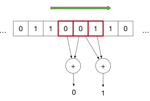
The convolutional encoder can be seen as a sliding window calculating n different
parities in parallel. The sliding window receives a stream of bits as its input and calculates the outputs, as shown in Figure 1.2. In this example, there are 3 red squares, where the first reads the actual valuex[n], and the next 2 squares read the delayed valuesx[n−1]andx[n−2].
Thus, there are two binary memories.
1
0
0
1
0
+
+
1
0
…
…
1
0
1
Figure 1.2: Representation of a convolutional code as parities on a sliding window.
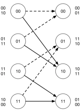
As the memory elements inside a binary convolutional code are limited only to the values 0 and 1, the code can be described as a finite state machine with 2m states, m being
the number of memory registers. This representation leads to a trellis diagram that can be used at the decoding procedure. The finite state machine can be described by a state diagram as shown in Figure 1.3. This diagram represents the same code of Figure 1.2, where each state is represented by the bits of the first memory and the second, in this order. A dashed line is an input bit 0 and a solid line is an 1. The outputs are represented by the two bits
y1[n] =x[n] +x[n−1]and y2[n] =x[n−1] +x[n−2], labeled next to the transitions. In this
diagram, it is hard to read a sequence of states along the evolution of time. A trellis diagram can represent time better, as it shows both all previous and next states at once. Figure 1.4 shows the same code as a trellis diagram.
00 01
10 11
10
01 11 11
00 01
10
Figure 1.3: State diagram.
00
01
00
10
11
01
10
11 00
10
01 11
11 01
10 00
00 01
11 10
10 11
01 00
data in a stream-like fashion, generating just one big codeword. Furthermore, the decoding can also be performed in the same fashion, which can reduce the latency caused by waiting the full codeword to be received.
1.2
Reed-Solomon codes
Reed-Solomon codes are a powerful class of error correction and detection non-binary codes. The main focus of Reed-Solomon is to have control over the error correction capabilities of the code. It operates on polynomials over finite fields.
In order to generate a Reed-Solomon code, one must define a finite field. A finite field can only have a prime power as its number of elements, so typically 2 is used as the base
prime, resulting in fields of order q = 2m. In this work, m = 8 is conveniently used, in order
to make a field with 256 elements, which we can represent using 8 bits, a byte.
After setting the finite field, the codeword length of the code isNRS =q−1 symbols. A symbol can be any element from the field. Now we must set the number of parity symbolsMRS.
By construction, a Reed-Solomon code can correct up to half the number of parity symbols in a codeword. The number of information symbols is KRS = NRS −MRS. For example, we
can use MRS = 32 parity symbols resulting in a codeword of KRS = 255−32 = 223, so that
we have a (255,223) Reed-Solomon code.
A Reed-Solomon code can be viewed as an interpolation problem, as follows: given two different polynomials with KRS coefficients, we evaluate them at the same NRS points. Now
these points agree in at most KRS −1 points. This is because if they agree in KRS points,
one could interpolate them and generate the same polynomial, contradicting the premise that they are different. If they agree in at most KRS −1 points, they disagree in at least NRS −(KRS −1), resulting in a minimum distance of d = NRS −KRS + 1, so that we can
correct up to t =⌊d−1 2 ⌋=⌊
NRS−KRS
2 ⌋erroneous symbols. In this case, the decoding algorithm
must find a way to find the errors such that the interpolation of the values can return the polynomial. The evaluation points usually are taken as consecutive powers of a primitive element α: α0,α1,α2,. . ., because this leads to interesting mathematical properties.
Another view, adopted from BCH codes, is that a Reed-Solomon codeword itself is a polynomial of NRS coefficients. The requirement is that this codeword is divisible by the
G(X) = Y
i=1
(X−αi) = X
i=0
giXi , (1.2)
where a codeword is any polynomial with NRS coefficients divisible by G(X). In other words,
a codewords has at least the same roots of G(X). A systematic encoding algorithm finds a codeword that starts by the given message and calculates the rest by making the codeword divisible byG(X). In order to do this, one should fill the coefficients of the codeword from the highest order coefficients, leaving the lower ones as zeros, then after calculation of the remain-der of the polynomial division, we subtract this remainremain-der and thus generate a polynomial divisible by G(X).
(1.4) shows the equation for this method, where M(X) is the message polynomial, with its coefficients conveying the information, R(X) is the parity polynomial, and C(X) is the codeword constructed by the concatenation of M(X)and −R(X).
R(X) = M(X)XNRS−KRS modG(X) (1.3)
C(X) = M(X)XNRS−KRS−R(X) (1.4)
Both views seems very different as in the first we evaluate a polynomial to obtain the values as a codeword, and in the second the codeword is a polynomial itself. If we consider that we evaluate the polynomial of the first view at consecutive powers of α,αi, i = 0,1,2, . . . , NRS−1 , we can relate both views by the finite field Fourier transform. From
the first view, we have a polynomial
c(X) =c0+c1X+c2X2+· · ·+cKRS−1X
KRS−1 (1.5)
and then we evaluate c(X) at αj, in order to calculate the codeword Cj =c(αj), resulting in
a familiar formula
Cj =
NRS−1
X
i=0
ciαij, (1.6)
also, the inverse transform is valid, ci = N1
RSC(α
−i) = 1
NRSC(α
NRS−i), resulting in ci = 1
NRS NRS−1
X
j=0
Cjα−ij
= 1
NRS NRS−1
X
j=0
Cj(αNRS−i
)j, (1.7)
where 1/NRS is the reciprocal of
NRS
z }| {
1 + 1 +· · ·+ 1, which, in the binary case, equals to 1, and
alsoαN
RS = 1. From (1.5) and (1.7) we can note that ci = 0 for i=KRS, KRS+ 1, . . . , NRS−1,
so thatC(αNRS−i) = 0for the samei’s, or equivalently, C(αk) = 0fork = 1,2, . . . , N
RS−KRS.
1.2.1
Finite fields
The definition of a finite field, in a few words, is a kind of “interface” (from program-ming languages), that is, it is a set that satisfies some requirements (methods or function, in a programming language), so that these requirements are sufficient for us to use other tools. Basically, a finite field is a finite set with two operations, namely addition and multiplication, and both are invertible inside the field. The most notable (non-finite) field would be the ratio-nals Qrepresenting fractions of integers, on which can be performed the four basic arithmetic
operations.
The requirements of a field enable us to use all the mathematical knowledge that already works on sets such as C, R and Q on other sets, even sets we define ourselves. For example,
algebra tools used for system of equations, polynomials, matrices and vectors can be used on finite fields with minimal or no changes.
Formally a finite field is a set of elements, equipped with two operations, namely "addi-tion" and "multiplica"addi-tion". The quotation marks indicates that they are not the conventional addition and multiplication. They can be any operation, usually defined conveniently to serve a purpose. A finite field requires closure of both operations, in other words, the "addition" and "multiplication" of two elements must result in another element in the set. Also, both operations have a identity element, namely "0" and "1" (note the quotation marks again), where "0" is an element such that a+ 0 =a and "1" is an element such that a·1 =a. Also,
both operations have the associativity and commutative properties, meaning that the order each operation is carried does not matter. Another required property is that the "multiplica-tion" is distributive over "addi"multiplica-tion", a·(b+c) = ab˙+ac˙. And the last requirement is what
differs a field from a commutative ring, which is the presence of inverses for both operations, as a commutative ring requires inverses only for "addition". An inverse of a element for an operation is another element which when applied the operation gives a identity element. For example, for "addition" b is the additive inverse of a when a+b = 0, usually we explicitly name b asb =−a, such thata+ (−a) = 0. The same goes for "multiplication", c·d= 1, and
we express d as d = 1c, such that c· 1c = 1. An exception for the inverse requirement is "0",
which has no multiplicative inverse. The field we usually learn first is the set of rationals Q,
where we can divide any number. The reals R and complexes Care also fields.
A finite field is a field with a finite number of elements. Considering that the "0" and "1" are different, 0 6= 1, the smallest finite field we can construct is using addition and
+ 0 1
0 0 1
1 1 0
× 0 1
0 0 0
1 0 1
subtraction are equal, as 1 + 1 = 0.
It is possible to construct any finite field with a prime number of elements using the same method of considering addition and multiplication modulo p, wherep is prime. Furthermore, it is possible to construct finite fields with its number of elements equals to a prime powerpn,
but using a different method. This method uses primitive polynomials over base prime fields instead of prime integers, such that the field elements are now represented by polynomials. Primitive polynomials are the minimal polynomials of primitive elements. Primitive elements are generators of the field multiplicative group, which is cyclic (excluding 0). In other words, if we take one root of a primitive polynomial and apply consecutive powers to it, we obtain the entire multiplicative group, generating the entire field.
As an example, to generate the finite field of 4 elements, we use polynomials with two coefficients from the binary finite field. The primitive polynomial is given as X2+X+ 1, and
the elements of the field are calculated modulo this polynomial. This results in four possible polynomials, with degree up to 1. The polynomials are 0, 1, X and X+ 1. Considering α as
one of the roots of X2+X+ 1, then
α2+α+ 1 = 0 (1.8)
α2 =α+ 1 (1.9)
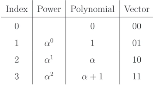
and the field is {0,1, α, α2}, or equivalently,{0,1, α, α+ 1}, or in binary form {00,01,10,11}.
One can note that α can be both X orX+ 1, but this does not matter, the field operations will behave the same. We showed three different views of this field, resumed in Table 1.2
To perform addition, we just use the polynomial view and add coefficients of same degree. This is also equivalent to a XOR operation between their vector representations. In the other side, for multiplication, we use the power representation and just add the exponents modulo 3 (the exponents can be only 0, 1 or 2, in this example). This said, Table 1.3 shows
both addition and multiplication tables, proving that this construction is indeed a field, as this set is closed under both operations, and each line and column has the respective identity element, indicating the presence of inverses.
Table 1.2: Three different views of GF(4). Index Power Polynomial Vector
0 0 00
1 α0 1 01
2 α1 α 10
3 α2 α+ 1 11
Table 1.3: Addition and multiplication tables for GF(4). + 0 1 α α2
0 0 1 α α2
1 1 0 α2 α
α α α2 0 1
α2 α2 α 1 0
× 0 1 α α2
0 0 0 0 0 1 0 1 α α2
α 0 α α2 1
α2 0 α2 1 α
selecting a higher degree primitive polynomial.
1.2.2
Encoding
Reed-Solomon [2] encoding can be performed in numerous ways. Using the interpola-tion view, we assume that the informainterpola-tion to be encoded is a polynomial and evaluate this polynomial of degree up toKRS−1atNRS different points. The evaluation points usually are
taken at consecutive powers {α1, α2, . . .} of a primitive elementα as this leads to interesting
mathematical properties. This leads to a non-systematical encoding, where the information is not directly available on the codeword.
A way to encode systematically, using the same interpolation view, is to directly set the first values of the codeword as the information to be encoded, in other words, forcing the codeword to be systematic. To calculate the remaining parity values, we interpolate the
KRS information symbols in order to make a polynomial and evaluate this polynomial at the
remaining NRS−KRS positions. This method implies more cost due to the interpolation, but
on the other hand it results in a systematic encoding procedure.
Using the BCH [11] view, we have a generator polynomial G(X), and a codeword is
where C(X) is guaranteed to be a multiple ofG(X). Again, this does not yield a systematic encoding.
For a systematic encoding using the BCH view, one must force the first coefficients of
C(X) to be the information symbols by doing M(X)X(NRS−KRS), this leaves the coefficients
of smaller degree set to 0. Now, to make a codeword, C(X) must be a multiple of G(X), so we have to subtract the amount it needs to be a multiple, thus we subtract the remainder of the polynomial division of M(X)X(NRS−KRS) by G(X). As a result we have that C(X) =
M(X)X(NRS−KRS) −(M(X)X(NRS−KRS) modG(X)). One can make an analogy to integers,
for example, if we want a multiple of 7, we could take any number, say 52, and then take 52 mod 7 = 3, then we just subtract 52−3 = 49, which is a multiple of 7. Note that this is the very definition of remainder of division.
1.2.3
Decoding
Reed-Solomon decoding, ideally, could be made using interpolation, as one can inter-polate all the combinations of the received NRS values, taken KRS at a time, and then create
a ranking counting which polynomial appears more frequently, this would be the decoded polynomial. While the idea is simple, it is costly due to the combinatorics explosion even on smaller codeword lengths.
In order to decode efficiently, a syndrome decoding method was devised. This greatly reduces the cost, as we work only with syndromes, ignoring the codeword entirely. The syndrome sizes are as big as the redundancy sizes, so usually their lengths are only small fractions of the codeword lengths.
Assuming T(X) is the transmitted polynomial, R(X) is the received polynomial, and
E(X) is the error polynomial, such that
R(X) = T(X) +E(X), (1.11) we have that T(X) is codeword, thus T(X) have at least the same roots as the generator polynomial G(X), resulting that T(αi) = 0 for i = 1,2, . . . , N
RS −KRS. Knowing this, we
have that
where Si represents the syndrome for each value of i. Now, considering polynomial E(X)
having only t errors, we have
Sj =E(αj) = t X
k=1
eik(α
j)ik, (1.14)
where ik is a index at E(X) where coefficient eik is non-zero. Considering Zk = α
ik as the
error locations and Yk=eik as the error values, we have Sj = t P
k=1
YkZkj, which can be seen as a system of equations:
Z1 Z2 . . . Zt
Z2
1 Z22 . . . Zt2
... ... ... ...
Zn−k
1 Zn
−k
2 . . . Zn
−k t Y1 Y2 ... Yt = S1 S2 ...
Sn−k . (1.15)
The main decoding problem is to find theZk, corresponding to the leftmost matrix. Note that
this is a overdetermined system, which can lead to multiple solutions. The true solution is the one which minimizes t, in other words, which assume a minimal number of errors.
Finding the error locations Zk are by far the most complex part of decoding. This can
be done by using the Berlekamp-Massey [12,13] algorithm. This algorithm is used to calculate the error locator polynomial, which is defined as polynomial Λ(X) which has the reciprocals
Z−1
k as its roots:
Λ(X) =
t Y
k=1
(1−XZk), (1.16)
and Λ(Z−1
k ) = 0. Using the algorithm, we find Λ(X), and then we can calculate its roots by
exhaustive search, which is feasible as it is a polynomial over a finite field. This exhaustive search is done efficiently by an algorithm called Chien search. With Zk calculated one can
finally calculate Yk by solving (1.15). Again, there is a efficient algorithm called Forney
algorithm which calculates Yk. With both Zk and Yk, we construct E(X) and recover T(X)
by just subtracting T(X) =R(X)−E(X).
1.3
Trellis-coded modulation
Trellis-coded modulation is a technique that mixes both a convolutional code and a modulation scheme. The key concept of this technique is to replace conventional Hamming distances between sequences of bits by Euclidean distances between sequences of constellation points. A typical trellis-coded modulation is done by using a convolutional code of rate k
to a 8-PAM constellation. Considering an uncoded modulation, this expansion would reduce
the distance between any two neighboring points, assuming the same transmission power. The advantage of coded modulation is that we do not consider the neighborhood anymore as the code design ensures that the only possible points are farther than the closest neighbors, thus increasing the distance.
In practice, trellis-coded modulation uses uncoded and coded bits. For example, using a 256-QAM modulation, each symbol contains 8 bits. Using a hierarchical constellation map-ping, we could assign different importances to each bit. In other words, it means that some bits are more susceptible to noise than others. As an example if a bit is the only difference between two neighbor points, then this bit is very fragile to noise, as opposed to the situation where a bit defines the quadrant or the sign of a constellation point. The strategy used by trellis-coded modulation is to protect fragile bits using convolutional codes, and leave more robust bits uncoded. This leads to a very efficient scheme where we can produce coding gains by sacrificing just one bit as redundancy. For a concrete example, Chapter 2 has a detailed implementation of a trellis-coded modulation scheme.
1.3.1
Encoding/Mapping
The encoding of trellis-coded modulation is pretty straightforward: we just feed the input bits to the convolutional encoder to generate the output bits, then these bits are mapped to the respective points in the constellation. These steps have no difference from a non-coded modulation scheme, as the difference lies in the fact that the design of the code is fully aware of the mapping of the constellation points, thus taking in account which output bit pattern generates each point. The design is made by maximizing the (Hamming) distance between sequences of bits, and then each bit pattern is mapped accordingly into the constellation in or-der to maximize the (Euclidean) distance between points, in other words a good convolutional code may not have the same performance when used for trellis-coded modulation, because it depends on the modulation scheme used.
1.3.2
Decoding/Demapping
likelihood decoding is well-known as the Viterbi algorithm. The Viterbi algorithm finds the best sequence of constellation points that minimizes the overall Euclidean distance checking all possible sequences in a clever way that greatly reduces the complexity. The main decoding scheme is made in a similar way as of a conventional convolutional code, which is composed by three parts. The first one is the branch metric unit, which, in the trellis-coded modulation, calculates the branch metrics for each output pattern by looking at the constellation and returning the Euclidean distance metric. Then, the second part is the path metric unit, which uses the Viterbi algorithm to determine the sequence of states and branches that minimize the path total Euclidean distance. Finally, the last part is the traceback unit, which just follow the trellis backwards from the last state, backtracking the path with minimum distance and returning the input that generated this path. The input is then the decoded message.
1.4
Low-Density Parity-Check codes
Low-Density Parity-Check (LDPC) [4, 14, 15] codes are iterative block codes, used as an error correcting code. LDPC codes are defined by a parity check matrix, which represents a bipartite graph. The main characteristic is that the parity check matrix has to be sparse, that is, it contains a low number of non-zero values.
As a linear code, an LDPC code has message lengthk and codeword lengthn, defining
a (n, k) LDPC code. The parity-check matrix H is a (n−k)×n sparse matrix. A codeword is any vector ˆv that satisfiesvHˆ T = 0.
The design of a LDPC code is generally done using random or pseudo-random tech-niques to generate H.
1.4.1
Encoding
LDPC codes can be encoded, in general, as a linear code, multiplying the message vector by a generator matrix. To find a systematic encoding procedure, one can apply Gaussian elimination on H in order to obtain an identity matrix at the right side ofH. With H in the
form [ P In−k ], we find generator matrix G using G= [ Ik −PT ]. Although this method
works for all full rank matrices, the storage of G, and the multiplication uGˆ are problems as
G is not guaranteed to be sparse.
1.4.2
Decoding
Decoding is the difference between classical codes and iterative codes. LDPC decoding is done by receiving information from the channel and improving this information iteratively, until convergence to a valid codeword.
Decoding represents H with a Tanner graph, where each row is check-node, and each
column is a bit-node. Initial information from the channel enters the bit-nodes and flows through the connections of the graph to the check-nodes. Then the check node calculates new messages that flow back over the connections to the bit-nodes. The bit-nodes gather these messages and produces new messages again. This process is done until the messages converge to a valid codeword or the number of iterations is exceeded. This algorithm is called message passing, and it has a number of variants.
Standards Overview
This chapter provides a more detailed view of each code’s implementation on this work based on their respective standards.
2.1
G.fast forward error correction
The G.fast standard establishes new directives for broadband transmission on copper wires, allowing for connections speeds of up to 1Gbps. The FEC scheme for G.fast was chosen to be a combination of Reed-Solomon and trellis-coded modulation, which is a similar scheme to that of previous DSL standards [17].
2.1.1
Reed-Solomon
G.fast uses a Reed-Solomon code over GF(256). The codeword sizeNRS has a maximum value of 255bytes, which represents the code without shortening. With the use of shortening,
the minimum NRS is 32bytes. The redundancy size RRS can assume any even values from 2
to 16. The standard uses the primitive binary polynomial x8+x4 +x3 +x2+ 1 to perform
the arithmetic operations on GF(256).
2.1.1.1 Encoding
The encoding procedure seeks to implement
C(X) =M(X)XRRS modG(X), (2.1)
The multiplication by XRRS is used only to ‘make room’ for the RRS redundancy
sym-bols. As any codeword is divisible by G(X), we takeM(X)XRRS and calculate the remainder
of the polynomial divisionC(X). ThenM(X)XRRS+C(X)is divisible byG(X), which
guar-antees that it is also a codeword. Note that the codeword is just a concatenation ofM(X)and
C(X), resulting in a systematic encoding procedure. Systematic codes are preferred as, after the syndrome calculation at the decoder, if there are no errors, one should just drop C(X)to
recover the transmitted message.
The implementation basically is focused on the calculation of the polynomial division remainder. This can be done by using a digital filter over GF(256)in direct form II transposed, on which the remainder will be located at the filter memory. The division B(X)/A(X) can
be calculated by finding the impulse response of a digital filter H(X) = B(X)/A(X). In
this implementation, we exchange the positions of the impulse and the numerator, so we use
H(X) = 1/A(X) and the input are the coefficients of B(X). Also, each polynomial is read
from the greatest order coefficient, so that the trailing zeros of B(X) can be ignored and
A(X) first coefficient is 1. This can be done considering a temporary change of variables like
X =Y−1. The resulting encoding filter is shown in Figure 2.1. The message polynomial is the
inputx[n], the generator polynomial coefficients are multipliers, and the result is found at the memories of the delay line represented by the square blocks. Also, normally, the coefficients of G(X) should have changed their signs, but for finite fields with characteristic 2 we know
that a =−a for any a. 2.1.1.2 Decoding
The decoding procedure has, by far, the most computational cost. It is the decoder that has the intelligence of the code. The decoder has to decide whether errors are present or not, and, if there are errors, decide again whether the codeword can be corrected or not. If the number of errors exceeds the error correction capabilities of the code, then the decoder does not try to correct anything and return an error code.
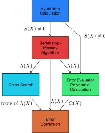
The decoder is implemented by the following main parts: syndrome calculation, Berlekamp-Massey algorithm, Chien search, error evaluator polynomial and error correction, as shown in Figure 2.2.
z−1
z−1
z−1
z−1
z−1
z−1
+ +
+ + + +
gRRS−1
gRRS−1
gRRS−2
gRRS−2
g0
g0
x[n] x[n]
Figure 2.1: Reed-Solomon Encoding Filter.
Syndrome Calculation
Berlekamp-Massey Algorithm
Chien Search
Error Evaluator Polynomial Calculation
Error Correction
Figure 2.2: Decoder blocks.
have the syndrome polynomial S(X), on which each coefficient is the value obtained for each
root. If all coefficients are zero, S(X) = 0, then the received polynomial is a valid codeword
and the algorithm stops, returning it as the decoded codeword. If S(X)6= 0, then at least one coefficient is non-zero, which means that at least an error occurred somewhere.
After knowing that at least an error exists, we must determine three things: the quantity of errors, the location of errors and the value of errors. The Berlekamp-Massey algorithm calculates the error locator polynomial Λ(X)which has as its roots the reciprocal of the errors locations, so that finding the roots of the polynomial results in finding the error locations.
To solve the Λ(X) polynomial, we must find all possible roots. This is accomplished by testing all possible values and looking for the ones that results in 0. This testing procedure
can be implemented using Chien search to reduce the number of calculations. Chien search then returns the locations of errors.
As this code is not binary, one also needs to calculate the values of the errors, which is done by firstly calculating the error evaluator polynomial Ω(X). Ω(X) is calculated by Ω(X) = S(X)Λ(X) mod XRRS, which means that each coefficient from Ω(X) is obtained by
convolution of the coefficients of Λ(X) and S(X), up to the (RRS −1)-th degree coefficient. Having access to Λ(X), to its roots and to Ω(X), we can use Forney algorithm to find the values of the errors using
ej = rj
−1Ω(rj)
Λ′(rj) (2.2)
where ej is error value, rj is the root associated to ej and Λ′(X) is the formal derivative of
Λ(X). The formal derivative in a field of characteristic 2is quite simple, as the coefficientsλ′
i
are determined by:
λ′
i =
λi+1 if i is even
0 if i is odd
(2.3)
then, finally, to apply the correction we just add each error value ej on its respective location rj−1. This completes the decoding process returning a corrected message as its result.
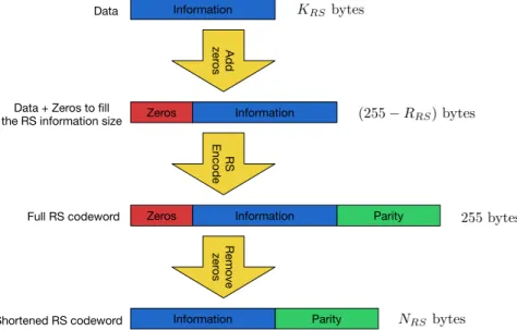
2.1.1.3 Shortening
The shortening procedure is used to reduce the fixed codeword size of 255 by inserting zeros as information bytes. For NRS bytes we have an amount of zeros A0 = 255−NRS. The
redundancy size RRS is not modified, so effectively the code rate drops as we are reducing
not transmitted, as the receiver already know that this part is zeros. The main advantage of shortening is that we can change the code rate using exactly the same Reed-Solomon code.
Information Parity
Zeros Original RS codeword
Shortened RS codeword Parity
Parity Transmitted RS codeword
Information
Information
Figure 2.3: Shortening process.
Figure 2.4 shows each step of shortening. At first, we receive KRS bytes to be encoded. As the Reed-Solomon encoder uses 255−RRS bytes, we have to fill the difference with zeros.
The encoding process then calculatesRRS parity bytes to form a full Reed-Solomon codeword
with 255 bytes. At the last step, we remove the zeros to transmit only relevant information.
Zeros
Parity
Parity Information
Information Information
RS
Encode
A
dd
zer
os
Zeros Information
Remove
zer
os
Data
Data + Zeros to fill the RS information size
Full RS codeword
Shortened RS codeword
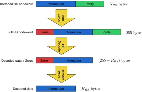
Unshortening does the reverse process of shortening, adding the zeros to reconstruct a full codeword. This procedure turns shortening invisible to the decoder, which interprets the zeros as information as well. The steps are shown in Figure 2.5.
Zeros
Parity Parity
Information Information
Information
RS
Decode
A
dd
zer
os
Zeros Information
Remove
zer
os
Shortened RS codeword
Full RS codeword
Decoded data + Zeros
Decoded data
Figure 2.5: Each step of Reed-Solomon decoding.
2.1.2
Interleaving
Interleaving is used to control error bursts. Error bursts are a sequence of errors occurring next to each other that easily overwhelm the error correcting capacity of the Reed-Solomon code. One of the main sources of error bursts is the trellis-coded modulation, given that the Viterbi decoder often produce this kind of errors. Interleaving is done by shuffling data in a way that bytes located near to each other before shuffling are located in different Reed-Solomon codewords after shuffling. The effect is that the errors are spread across several codewords, decreasing the probability of decoding failure on the Reed-Solomon decoder.
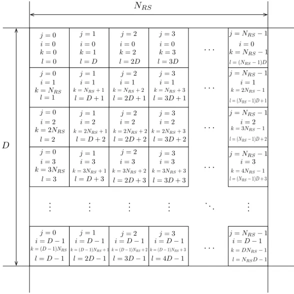
G.fast uses a block interleaver which is implemented using a matrix. This matrix has D
rows, representing the codewords, and NRS columns, representing the bytes of each codeword. D is called interleaver depth and D= 1 means no interleaving.
calculate the output position l using
l =j×D+i, (2.4)
wherel vary from0toNRS×D−1. iand j can be calculated from the input position k using
i=k/NRS, (2.5)
where / is integer division, and
j =k modNRS, (2.6)
such that k = i×NRS +j. Figure 2.6 shows the interleaving matrix with values for i , j , k and l. We can easily note that k increases following a row-wise fashion and, on the other
hand l increases following a column-wise fashion.
. . . . . . . . . . . . . . . . . . . . . . . . . .. . . . . . . NRS D
j= 0
j= 0
j= 0
j= 0
j= 0
j=1
j=1
j=1
j=1
j=1
j=2
j=2
j=2
j=2
j=2
j=3
j= 3
j= 3
j= 3
j= 3
j=NRS−1
j=NRS−1
j=NRS−1
j=NRS−1
j=NRS−1
i= 0 i= 0 i= 0 i= 0 i= 0
i=1 i=1 i=1 i=1 i=1
i=2 i=2 i=2 i=2 i=2
i= 3 i= 3 i= 3 i= 3 i= 3
i=D−1 i=D−1 i=D−1 i=D−1 i=D−1
k= 0 k=1 k=2 k= 3 k=NRS−1
k=NRS
k=2NRS
k= 3NRS
k= 3NRS−1
k=2NRS+ 1 k=2NRS+ 2 k=2NRS+ 3
k=2NRS−1
k=NRS+ 3
k=NRS+2
k=NRS+1
k=(D−1)NRS k= (D−1)NRS+ 1k= (D−1)NRS+ 2 k= (D−1)NRS+ 3 k=DNRS−1
k= 3NRS+1 k= 3NRS+ 2 k= 3NRS+3 k=4NRS−1 l= 0
l=1
l=2
l= 3
l=D−1
l=D l=2D l= 3D l= (NRS−1)D
l=D+1
l=D+2
l=D+ 3
l=2D−1 l= 3D−1 l= 4D−1 l=2D+ 1
l=2D+ 2
l=2D+ 3
l= 3D+1
l= 3D+ 2
l= 3D+ 3
l= (NRS−1)D+ 1
l= (NRS−1)D+ 2
l= (NRS−1)D+ 3
l=NRSD−1
Deinterleaving just does the inverse process of interleaving using the same matrix, but this time we write the input bytes column-wise and read them row-wise. The output position
l can be calculated into a similar way as the interleaver, using indexes i and j:
l=j×NRS +i (2.7)
and also, iand j can be calculated from the input indexk using
i=k/D, (2.8)
where / is integer division, and
j =k modD (2.9)
such that k =i×D+j.
2.1.3
Trellis-coded modulation
G.fast trellis-coded modulation is the same as previous DSL standards, which use a Wei’s 16-state 4-dimensional trellis code.
2.1.3.1 Bit extraction
Bit extraction is the way we take bits in order to apply trellis-coded modulation given a bit allocation table (bitload). In this work, we used only modulations with an even number of bits, so that the bitload is limited to even values. This is because these constellations mapping algorithms are easier. G.fast uses a 4-dimensional trellis code, which in turn uses 2 2-dimensional (QAM) constellations, meaning that the trellis code sees two sub-carriers as one. This has the effect that the bitload is read in pairs formed by consecutive entries in the bitload.
In order to fit the bitload exactly, for each sub-carrier pair(x, y), we extractz =x+y−1
bits. The 1 bit difference accounts for the redundancy bit introduced later by the encoder.
For the last two pairs, only z =x+y−3 bits are extracted. These 2 extra bits are used to force the encoder to return to its initial all-zero state.
The z bits form a binary word uˆ, which can be represented in two forms, according to the two cases above: if the pair is not one of the last two pairs, then uˆ ={d1, d2, . . . , dz}. If
and b1 and b2 are the extra bits mentioned above. Note that the length (len) of uˆ changes in
each case, being len(ˆu) = z in the first case and len(ˆu) = z+ 2 in the second case.
There is a special case when the bitload has a odd number of entries. In this case we insert a dummy entry with value 0 to make the number of entries even. Also, uˆ =
{0, d0,0, d1, d2, . . . , dz −1} to fill the dummy sub-carrier with zeros.
2.1.3.2 Encoding
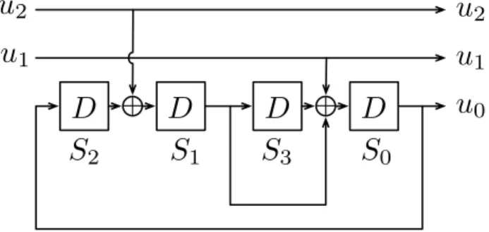
G.fast uses a convolutional code described in the finite state machine of Figure 2.7. This representation is useful for the encoding operations, as we can just implement the state machine with XOR and AND operations on the input bits.
D
+
D
D
+
D
u
1u
2u
1u
2u
0S
0S
1S
2S
3Figure 2.7: Finite state machine form of the trellis code.
The rate2/3systematic recursive convolutional code takes 2inputsu1 andu2 and
gen-erates a parity bit u0 based on the inputs and its internal memory. As the code is systematic,
the input bits are repeated at the output as well.
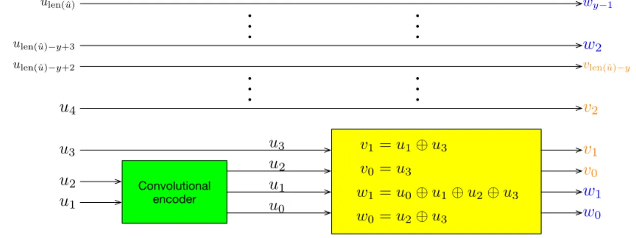
The encoder receives the binary worduˆ, adds1bit at the beginning (u0) and calculates
two binary words vˆand wˆ, with lengths x and y, respectively. To calculate u0, we take only
the first two bits u1 and u2 and input them on the convolutional encoder. Then, to calculate
ˆ
v and wˆ, we take the three bits from the output of the convolutional encoder plus an extra uncoded bit u3 and input them to the bit converter, which produces four bits (v0, v1) and
(w0, w1). These are the first two bits for each binary word, the other bits are uncoded bits
taken directly from uˆ. The bits from v2 to vlen(ˆu)−y are taken from u4 toulen(ˆu)−y+2. The bits
Convolutional encoder
v1 =u1⊕u3
v0 =u3
w1 =u0⊕u1⊕u2⊕u3
w0 =u2⊕u3 w0
w1 u1 u2 u3 u0 u1 u2 u3 u4
.
.
.
.
ulen(ˆu)−y+2
ulen(ˆ
u)−y+3
vlen(ˆ
u)−y w2
.
.
.
.
v0 v2 v1b
it conversion
Figure 2.8: Relation ofuˆwith vˆand wˆ. 2.1.3.3 QAM modulation
Although QAM modulation is not an error correction code, we had to implement it in order to have a baseline system. G.fast QAM design has trellis-coded modulation taken in consideration, so that it is not Gray-coded, for example. In other words, these constellations are best used with trellis-coded modulation, and have suboptimal bit error rates otherwise.
The modulation algorithm is simple for even number of bits b = log2(M), where M is
the modulation order. To calculate integer coordinates x and y one should just assign bits
alternately to x and y. The MSBs are interpreted as the sign bit, and the other bits are interpreted assuming a two’s complement form. Assuming vˆ = {vb−1, vb−2, . . . , v0} are the
bits to be modulated, xˆ={vb−1, vb−3, . . . , v1,1} and yˆ={vb−2, vb−4, . . . , v0,1} are the binary
representations in two’s complement form of x and y, respectively. For example, if we are considering 16-QAM, then b = 4 bits, supposing these 4 bits are ˆv ={1,0,1,1}, we have that
ˆ
x = {1,1,1} = −1 and yˆ = {0,1,1} = 3, forming the point (−1,3). Figure 2.9 shows an example for b= 8.
This algorithm makes the two LSBs of each point form 4 grids with minimal distance of 4 instead of 2 if we are measuring distances only from the same grid. Figure 2.10 shows
v
0v
1v
2v
3v
4v
5v
6v
7v
7v
5v
3v
1v
6v
2v
0v
41
1
b
=
8 bits
ˆ
x
y
ˆ
odd even
Figure 2.9: Modulation algorithm.
1
3
1
3
1
3
1
3
0
2
0
2
0
2
0
2
1
3
1
3
1
3
1
3
0
2
0
2
0
2
0
2
1
3
1
3
1
3
1
3
0
2
0
2
0
2
0
2
1
3
1
3
1
3
1
3
0
2
0
2
0
2
0
2
4
2
Figure 2.10: 2-dimensional cosets in a QAM constellation. 2.1.3.4 QAM demodulation
QAM demodulation is made differently, as the constellations are trellis-coded. For each received coordinate, we calculate the distance for each 2D coset, resulting in 4 distances. For
coset with index 0 C0
4D is formed by the union two Cartesian products. The first is between
the 2D coset of index 0 for the first subcarrier with the 2D coset of index 0 for the second
subcarrier. The second product is between the 2D coset of index3for the first subcarrier and the 2D coset of index3for the second subcarrier. To calculate the distance metric for this4D
coset, we have to do the following. Calculate the 2D distance from the received coordinates
of the first subcarrier to the nearest points that belongs to cosets 0 and 3. The same is done for the second subcarrier coordinates. Then, to calculate the 4D distances we sum the 2D
distances from coset 0 for both subcarriers, and the same for coset 3. Finally, we choose the
smaller4D distance as the candidate. Note that the distances are squared euclidean distances, which allows us to sum 2D distances to obtain 4D distances. Also, we should mention that
the Cartesian product corresponds to a sum of distances, while the union corresponds to a choice for the minimum. We must pair each distance with its respective bits. These bits are obtained by reversing the process described in Figure 2.9. This is basically “shuffling” the bits from the binary representation of the coordinates, putting the bits of x coordinate in the odd positions and bits of y in the even positions.
Given that a received point has coordinates R = (xr, yr), then to calculate the 2D squared euclidean distances to each 2D coset we just have to calculate the distance for the 4 nearest points, as shown in Figure 2.11. (xk, yk) is a point in 2D coset k and dk is the 2D
squared distance to 2D coset k, with k = 0,1,2,3. To calculate the 4D metrics, we need a pair of received points, thus the superscript < i > indicates which element of the pair we are
taking, 1 or 2. This generates 8 different distances, 4 for the first point, 4 for the second. Then we have to add distances from the first point with distance from the second, resulting in a 4D distance metric. These 4D metrics, with their respective possible candidate points, are passed to the Viterbi path metric unit.
The 4D cosets are formed according to the convolutional code, summarized in Figure 2.12.
From the above, we can summarize the demodulation steps as:
1. Receive coordinates as inputs
2. Find the 4 nearest points of each input, one for each 2D coset.
3. Calculate 2D square euclidean distances to 4 nearest constellation points
0 1 2 3 . . . . . . 0 1 0 0 2 d0 d1 d2 d3 . . . . . . 0 1 2 3 . . . . . . 0 1 0
0 d 2
0 d1 d2 d3 . . . . . .
First subcarrier Second subcarrier
d<1>
0
d<1>
1
d<1>
2
d<1>
3
d<2>
0
d<2>
1
d<2>
2
d<2>
3
D0=min(d
<1>
0 +d
<2>
0 , d
<1>
3 +d
<2>
3 )
D1= min(d
<1>
0 +d
<2>
2 , d
<1>
3 +d
<2>
1 )
D2= min(d
<1>
2 +d
<2>
2 , d
<1>
1 +d
<2>
1 )
D3= min(d
<1>
2 +d
<2>
0 , d
<1>
1 +d
<2>
3 )
D4= min(d
<1>
0 +d
<2>
3 , d
<1>
3 +d
<2>
0 )
D5= min(d
<1>
0 +d
<2>
1 , d
<1>
3 +d
<2>
2 )
D6= min(d
<1>
2 +d
<2>
1 , d
<1>
1 +d
<2>
2 )
D7= min(d
<1>
2 +d
<2>
3 , d
<1>
1 +d
<2>
0 )
dk=(xr−xk)2
+ (yr−yk)2
2D metrics
4D metrics
Figure 2.11: 2D and 4D distance metrics.
5. Take the minimum, according to the relations between 2D and 4D cosets summarized in Figure 2.12, also choosing the respective point from step 2.
6. The demodulator returns the possible pairs, with theirs respective 4D metrics, as its output.
The demodulator receives the coordinates for each subcarrier as its input and, with the bitload, calculates the demodulation candidates for each pair of subcarriers along with its distance from the received coordinate. The information that is forwarded to the Viterbi decoder is the sequence of distances, in order to calculate the which of the candidate point of the constellation should be used, and their respective candidate points.
2.1.3.5 Decoding
To decode this trellis code, the optimal algorithm, given that the code has only16states
Figure 2.12: Relation between 2D and 4D cosets, from G.fast standard.
best result in a manageable complexity.
The Viterbi decoder is divided in three units: the branch metric unit (BMU), the path metric unit (PMU) and the traceback unit (TBU). The BMU is simply the demodulator, which calculates the squared Euclidean distances (metrics). The PMU searches for the best path in a trellis, calculating the path metrics by summing and comparing the branch metrics provided by the BMU, and also saving each of the decisions in the TBU. The TBU calculates the best path by using the best path metric and then backtracking each decision in order to form the best sequence of outputs (cosets) of the convolutional code. With the coset sequence, we can finally choose the correct candidates to obtain the binary sequence.
from the encoder’s state machine.
Figure 2.13: Trellis diagram from G.fast.
In order to implement a Viterbi decoder, one must calculate the path with the minimal accumulated metric, so we define a state metric which represents the best metric until this state. These metrics are initialized with zeros. Then, recursively, these state metrics are updated at each step by the recursion formula
Sj[t+ 1] = min
i (Sp(j,i)[t] +Bj,i[t]), (2.10)
whereSj[t]is the state metric for state j at stept,Bj,i[t]is the branch metric calculated at the demodulator for statej and inputiat steptandp(j, i)is a state such that when we are at state
p(j, i) and receive input i, we end in state j, in other words, state p(j, i) transitions to state
j when given an input i. Clearly, function p(j, i) is defined by the design the convolutional
code, and can be taken from Figure 2.13 as well. For example, p(2,1) = C, as when on state C, and receive input 1, result in state 2. To see the input, we just take the integer division by
2 of the labels, so that input 1 is label 2, which is the fourth transition from top, connecting
C to2.
With just the state metrics, we can only calculate the best path metric, but we can not reconstruct the path itself. So we need to store the decisions at each step as well. This is done by
Dj[t+ 1] = argmin
i
(Sp(j,i)[t] +Bj, i[t]), (2.11)
where Dj[t] is the decision at step t which lead to state j. Note that (2.11) is similar with (2.10), with the only difference being a argmin instead of a min.
The Viterbi algorithm runs for all step, and for each step it runs for all states. In the end we will have a state metricSj for each final stepj and a table of decisionsDj[t]along each
step t. With the best final state metric we can finally find the best sequence by calculating it backwards. This is done by the traceback unit, which sets the final state by taking the minimum state metric. However this is not necessary in our case, as the encoding procedure guarantees that the sequence always start and finish at state zero. From the final state we just recursively traceback the decisions in order to find previous states and inputs by
s[t−1] = p(s[t], Ds[t][t]), (2.12)
where sequence Ds[t][t] will retrieve the inputs, and sequence s[t] is the sequence of states.
With this information one can finally choose the best sequence of constellation points and truly demodulate points into bits, thus removing the redundancy of convolutional coding.
Table 2.1: Distance by 4-D cosets.
P0 P1 P2 P3
Coset Dist. Labels Dist. Labels Dist. Labels Dist. Labels
0 13 (11,3) 15 (52,4) 7 (15,19) 5 (4,0) 1 7 (11,1) 5 (52,6) 5 (8,18) 3 (15,1) 2 1 (9,1) 15 (54,6) 3 (10,18) 5 (5,1) 3 7 (9,3) 9 (49,7) 5 (10,24) 3 (14,0) 4 13 (11,0) 7 (52,7) 3 (15,24) 1 (15,0) 5 7 (8,1) 17 (51,6) 1 (15,18) 7 (4,1) 6 13 (9,2) 7 (49,6) 3 (13,18) 5 (5,2) 7 7 (9,0) 17 (49,4) 5 (13,24) 3 (5,0)
example, only the survivors paths are shown for simplicity. A survivor path is a path that was not discarded in the min/argmin process. The red path shows the traceback from final state
0. This diagram was constructed for a sequence of four pairs, thus there are four columns of
transitions and five columns of states. The numbers above each state are the states metrics for each state at each step. We can note that possibly an error occurred in the second pair, as there is a sudden increase in all state metrics. By returning to state zero we could avoid an error at the final state, as without this information we would choose for final state 2 instead of 0, as the former has smaller accumulated state metric.
We can see directly that the sequence state is {0,1,5,4,0}, and with help of Figure 2.13, we can find the respective 4D cosets as {2,3,5,4}and thus find the nearest pair of points
to these 4D cosets, thus completing the demodulation/decoding.
2.2
G.hn forward error correction
1 2 3 4 5 6 7 8 A B C D E F 9 1 2 3 4 5 6 7 8 A B C D E F 9 1 2 3 4 5 6 7 8 A B C D E F 9 1 2 3 4 5 6 7 8 A B C D E F 9 13 13 1 28 20 20 6 10 18 18 28 28 20 22 18 30 30 20 9 13 9 11 15 15 15 21 21 21 23 23 19 21 21 1 2 3 4 5 6 7 8 A B C D E F 9 14 10 14 12 12 16 12 18 16 18 14 12 12 12 16
Figure 2.14: Viterbi algorith diagram example.