Design of New Materials for Passive Vibration Control

Abstract

The aim of this contribution is to extend the techniques of composite materials design to non-linear material behaviour and apply it for design of new materials for passive vibration control. As a first step a computational tool allowing determination of macroscopic optimized one-dimensional isolator behaviour was developed. Voigt, Maxwell, standard and more complex material models can be implemented. Objective function considers minimization of the initial reaction and/or displacement peak as well as minimization of the steady-state amplitude of reaction and/or displacement. The complex stiffness approach is used to formulate the governing equations in an efficient way. Material stiffness parameters are assumed as non-linear functions of the displacement. The numerical solution is performed in the complex space. The steady-state solution in the complex space is obtained by an iterative process based on the shooting method which imposes the conditions of periodicity with respect to the known value of the period. Extension of the shooting method to the complex space is presented and verified. Non-linear behaviour of material parameters is then optimized by generic probabilistic meta-algorithm, simulated annealing. Dependence of the global optimum on several combinations of leading parameters of the simulated annealing procedure, like neighbourhood definition and annealing schedule, is also studied and analyzed. Procedure is programmed in MATLAB environment.

Keywords: composite materials, passive vibration control, non-linear visco-elastic behaviour, optimization, shooting method, simulated annealing, cost functional.

1 Introduction

The latest developments in computational mechanics have lead to integrated methodologies that permit not only the structural design and shape optimization of the mechanical component but also the tailoring of the material properties and

Paper

166

Design of New Materials for

Passive Vibration Control

Z. Dimitrovová1 and H.C. Rodrigues2 1

UNIC, Department of Civil Engineering New University of Lisbon, Portugal 2

IDMEC, Department of Mechanical Engineering Technical University of Lisbon, Portugal

©Civil-Comp Press, 2009

consequently a design of new materials. This is particularly evident in the area of composite materials where the unit cell geometry (characterizing the composite material) is a key factor in its effective mechanical properties and thus can significantly improve the structural response of the mechanical component.

The aim of this contribution is to extend the techniques of composite materials design to non-linear material behaviour and apply them for design of new materials for passive vibration control. Objectives of the passive vibration control typically cover attenuation of the steady-state regime of the structure dynamic response. Then, at relatively low excitation frequencies is it important to reduce the steady-state displacements amplitude, which is generally obtained by an isolator of a strong material that may exhibit a low damping. On the other hand, at high excitation frequencies, a good isolator performance means that when the transmissibility is low. Then the isolator must possess high damping properties, which usually implies a soft material. Materials exhibiting high stiffness as well as high damping are not common [1-2]. Efficient properties for passive vibration control can only be achieved in man-made composite materials. Two-phase composites composed of a stiff, low loss phase, and a compliant, high loss phase, can exhibit high stiffness combined with high loss, providing that the lower bounds (Reuss for Young’s modulus of effectively orthotropic or Hashin-Shtrikman for effectively isotropic composite material) are saturated. These bounds must be rewritten by dynamic correspondence principle of the theory of linear viscoelasticity [3]. Actually very low volume fraction of stiff component embedded in high damping matrix can significantly improve the properties, [2]. The figure in merit is E*tanδ, where

*

E is the “norm” of the complex modulus E*, and

( )

_{( )}

* E Re

* E Im

tanδ= , i.e. δ represents the delay phase angle in strain response with respect to the stress one, i.e. the efficiency of damping. Within the framework of linear viscoelasticity, tanδ is proportional to the energy loss per cycle.

According to [1], extreme damping can be achieved when negative stiffness phase is implemented. Mechanical components exhibiting the negative stiffness are usually modelled by mechanism allowing for the snap-through. This can be achieved by two-spring mechanism [4]. An additional vertical spring is usually added in order to meet the required stiffness and/or for the optimization purposes [5]. Recently, a quasi-zero stiffness isolation, i.e. the isolation where in the global response there is a plateau at the equilibrium force, becomes popular [6].

As a first step in achieving the objectives of this work a computational tool allowing determination of macroscopic optimized one-dimensional isolator behaviour was developed. Voigt, Maxwell, standard and more complex material models can be implemented [9]. Objective function considers minimization of the initial reaction and/or displacement peak as well as minimization of the steady-state amplitude of reaction and/or displacement. Complex stiffness approach is used to formulate the governing equations in an efficient way. Material stiffness parameters are assumed as non-linear functions of the displacement. Numerical solution is performed in the complex space. Special attention is paid to the initial conditions, because in the complex space the transient solution yields an unreal behaviour originated by the fact that excitation frequency is already a part of the complex modulus. Steady-state solution is obtained by an iterative process based on the shooting method and imposing the conditions of periodicity on known value of the period [4]. Extension of the shooting method to the complex space is presented and verified. Non-linear behaviour of material parameters is then optimized by generic probabilistic meta-algorithm, simulated annealing. Dependence of the global optimum on several combinations of leading parameters of the simulated annealing procedure, like neighbourhood definition and annealing schedule, is also studied and analyzed. Procedures are programmed in MATLAB environment [10].

Paper is organized as follows. In Section 2 problem statement is given. Simplifying assumptions are summarized and the cost functional is defined. Section 3 describes the techniques used for numerical implementation, namely the shooting method and the simulated annealing. Section 4 presents some of the results obtained. Paper conclusions are summarized in Section 5.

Results presented, although still related only to one-dimensional behaviour, facilitate the design of elastomeric cellular/composite materials with improved behaviour in terms of dynamic stiffness for passive vibration control. Future research will be directed to optimization of multidirectional properties, which will be used as target behaviour for design of cellular and/or composite viscoelastic materials. This application will have a direct and immediate impact on product design and development, especially in the design of new mechanical components such as engine mounts and /or new suspension systems.

2 Problem statement

2.1 Optimal one-dimensional behaviour

Figure 1: Problem scheme.

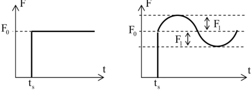
First of all it is necessary to state, what kind of excitation forces are included in the analysis. Load cases are chosen according to the realistic situations as: (i) step load, (ii) set of step loads, (iii) step load with harmonic component, (iv) set of step loads with harmonic components. Load cases (i) and (iii) are shown in Figure 2.

Figure 2: Schematic representation of load cases (i) and (iii).

Displacement u(t) as well as the time dependent reation R(t) have a transient and a steady-state part. The objective in the optimization problem is to minimize u(t) and R(t) amplitude in both regions. Thus the optimization problem for the load cases (i) and (iii), specified in Figure 2, can be stated as

find s

( )

t , such that ⎟⎟ ⎠ ⎞ ⎜⎜

⎝ ⎛

γ + γ

=

∈ ∈

∈

f r r

i t t;t

st st t ; t

t tr

tr s ~ s

1 min A A

O , (1)

where s~ is the design space of the isolators behavious, A and _tr A stand for the _st combination of maximum amplitudes of the displacement and of the support reaction in the transient and in the steady-state region, respectively. t_i, t_r and t_f

correspond to the initial time (from where the transient response gains importance

s

i t

t > ), to the transition time (from where the steady-state response gains importance) and to the final time of the analysis, respectively. In more details:

m

( )

t s

( )

t P

( )

t

u m

( )

t s

( )

t P

( )

t u

( )

t R

F

0

F

t

s

t

F

0

F

t

1

F

1

F

s

( )

( )

( )

( )

( )

( )

maxu

( )

t min u

( )

t , u 1 t R min t R max R A , t u min t u max u 1 t R min t R max R A f r f r f r f r r i r i r i r i t ; t t t ; t t st t ; t t t ; t t st st t ; t t t ; t t tr t ; t t t ; t t tr tr ⎟ ⎠ ⎞ ⎜ ⎝ ⎛ ₋ α − + ⎟ ⎠ ⎞ ⎜ ⎝ ⎛ ₋ α = ⎟ ⎠ ⎞ ⎜ ⎝ ⎛ ₋ α − + ⎟ ⎠ ⎞ ⎜ ⎝ ⎛ ₋ α = ∈ ∈ ∈ ∈ ∈ ∈ ∈ ∈ (2)

where α_tr, α_st express the importance of the reaction versus displacement in each of the considered regions and R , u are some convenient norms related to the particular problem. Further in Equation (1), γ_tr and γ_st are appropriate weights, highlighting the relative importance of each regime and with the property

1

st

tr +γ =

γ . Subscript “1” in the objective function O₁ means that only one single load case, (i) or (iii), is assumed. For step load according to (i), γ_st =0 can be taken because there is no steady-state response; for step load with harmonic component (iii) both weights γtr and γst can be non-zero. If only reaction contribution in

steady-state regime is considered, i.e. γtr =0, 1αst = , then one can assume

0

F 2

R = and thus min max R

( )

t min R

( )

t minT F 2 1 O s~ s t ; t t t ; t t s ~ s 0 1 f r f

r ∈ ∈

∈ ∈ ⎟⎠= ⎞ ⎜ ⎝ ⎛ ₋

= , where T is the

transmissibility.

Load cases (ii) and (iv) correspond to a set of discrete cases, where weights λ_i must be attributed according to the importance or to the probability of occurrence, and 1 r 1 i i = λ

∑

=

. Cost functional O is then defined as:

∑

= λ = r 1 i i i i O min

O , (3)

where r is the number of single load cases.

2.2 Simplifying assumptions and governing equations

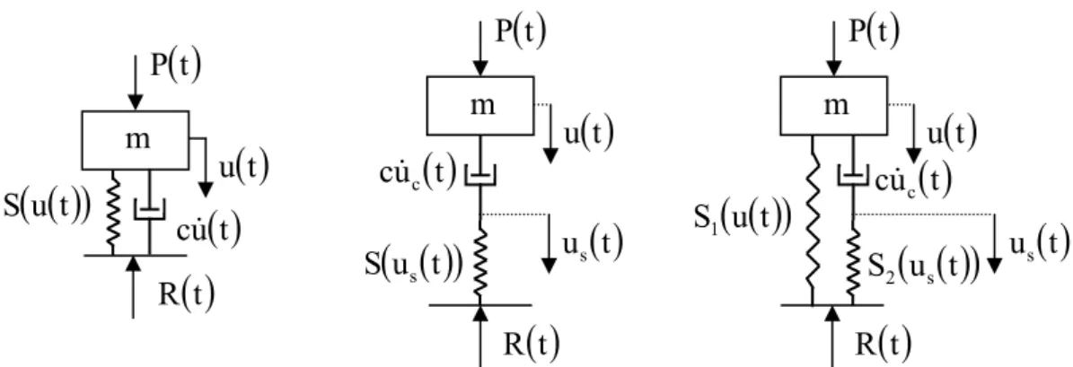
It is necessary to impose some simplifying assumptions on the isolator behaviour. As already mentioned in Introduction, it is assumed only one-dimensional behaviour. Particular material model can be the Voigt, Maxwell, standard or more complicated. In these cases the spring part is assumed non-linear elastic and the damped part linear is taken as viscous with a constant damping coefficient. Then the isolator can be schematically substituted as indicated in Figure 3, where S

( )

u

( )

t

Figure 3: Schematic representation of the isolator in form of Voigt, Maxwell and standard material model.

Equation of motion of the system from Figure 3 when Voigt model is assumed reads as, [11]:

( )

t cu

( )

t S

( ) ( )

u

( )

t P t mg u

m + + = + , (4)

where g is the gravity acceleration. Zero position of displacement can be shifted to the static equilibrium position if only mass is acting. Then:

( )

t cu

( )

t S

( ) ( )

u

( )

t P t u

m + + = , (5)

where for the sake of simplicity designation of the displacement is remained unchanged. Then the support reaction is given by:

( )

t cu

( )

t S

( )

u

( )

t

R = + . (6)

For other material models a system of equations must be written, [11]. For harmonic loading, however, it is then more convenient to introduce the concept of the complex stiffness, [9]. Then Equation (4) can be written as:

( )

( )

( )

( )

i t

Pe t u S t u ic t u

m + ω + = ω , (7)

where i the complex unity i= −1. In this representation Peiωt =P

(

cosωt+isinωt

)

. Regarding the steady-state final response, if originally the force applied was

t sin

P ω , then the imaginary part of the solution correspond to the final result, if t

cos

P ω was assumed, then the real part of the solution must be taken and if a general harmonic force was used, then the response corresponds to a combination of both parts. Following [9] it is easy to write the complex stiffness of any possible one-dimensional material model.

In order to characterize the design domain ~s , it is necessary to describe the allowable non-linear behaviour of the spring parts of the material models, i.e. the

m

( )

t P

( )

t u

( )

t u c

( )

( )

u t S

( )

t R

m

( )

t P

( )

t u

( )

t u c_c

( )

(

u t

)

S _s

( )

t R

( )

t u_s

m

( )

t P

( )

t u

( )

t u c_c

( )

(

u t

)

S_{2 s}

( )

t R

( )

t u_s

( )

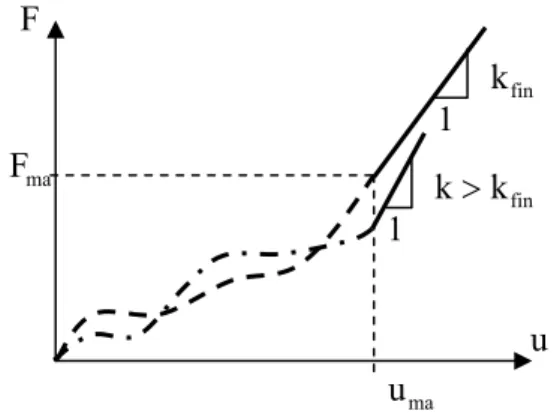
domain of admissible static curves. Practical applications require that spring rigidity is not arbitrary and that fixed and variable parts of the static curve must be identified. There is usually a final linear stage characterized by a rigid component, representing the alternative supporting system, which starts to actuate when the maximum allowable displacement u_ma of the flexible part is achieved. It is assumed, that the allowable displacement u_ma cannot occur later than the elastic force reaches the value F . Then in fact the final rigidity is not fixed but it is characterized by its _ma minimum value k_fin. Two possible designs of the non-linear spring are shown in Figure 4, variable (dashed) part of the static curve is the subject of optimization. It must be estimated by a convenient curve satisfying certain requirements in the interval 0,u_ma , namely:

a) Static curve must be continuous;

b) Static curve must be increasing, i.e. stiffness must be non-negative at any displacement value, in order to avoid dynamic instability;

c) Spring behaviour is perfectly hyperelastic, i.e. loading and un-loading paths matches exactly.

Figure 4: Two possible designs of the non-linear spring: fixed (full) and variable (dashed) parts of the static curve.

In order to determine the optimal static curve, an optimization procedure must be implemented. Generic probabilistic meta-algorithm, simulated annealing, was chosen for this purpose. The algorithm will be described in the next section. Besides the cost functional definition and simulated annealing general steps, several other procedures must be established, like the procedure for the variable part of the static curve definition. Then it is possible to solve the problem stated in Equation (5) numerically and evaluate the cost functional for such particular case. One of the possible approaches for the static curve definition is:

a) Select a set of fixed points u_i,i=1,...,n from the given open interval

(

0,u_ma

)

, assign 0u₀ = and u_n+1=u_ma (uniform distribution can be used Δu=u_i+1−u_i); b) Randomly select force values F_i,i=1,...,n+1 from the given interval

]

0,F_ma

]

,

order them in an increasing way and attribute them to the points u_i (F₀ =0);

fin

k 1

ma

u

u

ma

F F

fin

c) Define spline approximation within each interval u_i,u_i+1 ,i=0,...,n.

As far as the spline approximation, linear and cubic Hermite approximations were tested for suitability. Linear spline approximation is easy to implement, it preserves continues and monotonic behaviour, however it does not preserve stiffness continuity in the separation points u_i. Cubic Hermite approximation, on the other hand, establishes cubic polynomial approximation within each interval with continuity of the first derivative at u_i. Derivatives d_i at the separation points u_i can be given by finite differences, as forward, backward or centred approximation. Let

1 n

fin d

k = ₊ . Implementation of Hermite approximation is also straightforward, requirement a) is assured, however, requirement b), is not preserved.

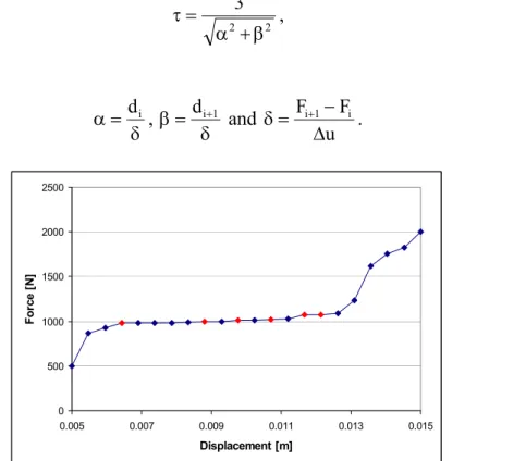
Monotonic behaviour is a crucial condition, therefore some adjustments must be implemented. Following [12], if the conditions for monotonicity are not met in a certain interval, derivatives at the end points of this interval, d_i and d_i+1, should be corrected to τd_i and τd_i+1, where

2 2

3

β + α =

τ , (8)

and

δ =

α di _,

δ =

β di+1 _and

u F F_{i 1 i}

Δ − =

δ + _{. (9)}

0 500 1000 1500 2000 2500

0.005 0.007 0.009 0.011 0.013 0.015

Displacement [m]

For

ce [

N

]

Figure 5: A possible choice of random forces. Red points identify the initial point of each interval where monotonicity conditions are not satisfied.

linear spline, red points mark initial end-points intervals, where at least one of the monotonicity conditions is not satisfied. Figure 6 shows the Hermite approximation within the first of these intervals determined by the original procedure (blue) and after the derivatives alteration (red).

977 978 979 980 981 982

0.0064 0.0066 0.0068 0.0070

Displacement [m]

For

ce [

N

]

Figure 6: Efficiency of the monotonicity criteria: Hermite approximation before (blue) and after (red) the derivatives alteration.

The two possible spline approximations described in this section were tested for accuracy and computational time. No significant differences were found in either of these criteria. Therefore the linear spline approximation is used in all examples presented in this paper because of its simplicity.

3 Numerical implementation

3.1 Shooting

method

method, Equation (5) must be written as a system of equations. Let us assume for the sake of simplicity that only one sinusoidal load is applied. Then:

( )

( )

( )

t

(

S

(

x

( )

t

)

cx

( )

t Psin t

)

/m, x t x t x 2 1 2 2 1 ω + − − = = (10)

where x₁

( ) ( )

t =u t and x₂

( ) ( )

t =u t . The shooting function h is defined as:

(

u ,u

) (

u ,u

)

, h : h T T 0 0 2 2 = ℜ → ℜ (11)

where T=2π/ω is the known period. The objective is to find the initial conditions

(

uF,uF

)

that ensure h

(

uF,uF

) (

= uF,uF

)

, i.e. h

( )

xF =xF. If x0 is an initial choice of

initial conditions, then the solution x_F can be found by an iterative procedure based on the Newton-Raphson method as:

( )

(

( )

n n

)

1 n n 1 n h h

I x x x

x x

x ⎟ ⋅ −

⎠ ⎞ ⎜ ⎝ ⎛ ∂ ∂ − + = −

+ . (12)

The crucial point in this process is to obtain the Jacobian matrix, i.e. the derivatives:

( )

( )

i,j 1,2 x h h _n j i n

ij _∂ =

∂

= x

x . (13)

Following [4] it is possible to prove, that these derivatives correspond to the solution of the linearized homogeneous system, expressed at the value of the solution of the previous step, when the base vectors are used for the initial conditions.

The methodology can be extended to the complex domain, then instead of 2x2 Jakobian matrix, 4x4 must be used. The advantage of the problem treated in this paper is that the original problem is already linearized.

3.2 Optimization

algorithm

Generic probabilistic meta-algorithm, simulated annealing, was chosen as optimization tool to solve the problem specified in Equations (1-3). In order to describe the optimization procedure let us assume for the sake of simplicity, that Voigt model is implemented and that at iteration k one has the respective static curve _S( )k _{and the objective function value O}( )k _{. Then for the next iteration (k+1) a}

(k 1)

S + is unconditionally accepted. If O(k+1) ≥O( )k then it can be conditionally accepted, based on the probability randomly selected from the interval

( )

0,1 and compared with the value calculated as exp

(

(

O( )k −O(k+1)

)

/T_j

)

, where T is the _j current cooling temperature. This criterion prevents the algorithm to stick at a local minimum and gives the possibility to search through the entire design domain. As the cooling proceeds, cooling temperature is getting lower and consequently the probability of acceptance decreases.

There are several crucial parameters in this algorithm which must be carefully chosen as they can distort the final result and/or make the calculation inefficient. They are:

a) The initial temperature;

b) The number of iterations within each temperature; c) The cooling schedule;

d) The stopping criteria;

e) The neighbourhood definition.

The initial temperature is usually defined as a ratio of the initial value of the cost functional. It should be stated in the way that the acceptance probability in the initial temperature stage is around 50%. The number of iterations within each temperature must be high, around 500 or more and must be adapted to each particular load case. It does not make much sense to implement many temperature levels, since then the probabilities of acceptance in two consequent temperatures will be very similar. The algorithm can stop before completing the cooling schedule, whenever the number of consecutive failures reaches the user-input number.

The neighbourhood definition is crucial in a simulated annealing algorithm. In our problem it is defined in percentage terms from the given static curve. In more details, user-input values are:

a) m≤n as number of forces which are allowed to vary;

b) p the percentage of variation related to the total allowable force value F . _ma After the new force values are obtained they must be ordered in an increasing way, in order to satisfy requirements specified in Section 2.2.

from the final optimal design was allowed and histogram of the objective function values for 1000 such simulations was analysed.

4 Obtained results

In this paper; the engine mount suspension system is considered as a practical application. Then, according to real solicitations, F has relatively high values, ₀ around 1000-2000N, and F₁ ranges about 1-2N with frequencies from 25Hz to 250Hz. Load case (i) stands for the action exerted on the engine in a sudden acceleration or a car stop. The harmonic contribution from load case (iii) represents the solicitation acting whenever the engine runs. Therefore, harmonic forces are always superposed to the step load. This means that load cases (i-ii) cannot occur in real applications, nevertheless they are worthwhile to study in order to draw conclusions about their particular influence. Voigt model is assumed, α_tr =α_st =1 and R =1. In this case the objective function has the unit of force.

Now, limitations of the static curve according to Figure 4 can be established numerically. Final part of the curve is limited by the maximum admissible displacement of the flexible part of the support, approximated by u_ma =10mm. In a standard rubber material this value corresponds to the applied load of F_ma =1500N. After that rigid components of the support start to actuate, thus the system obeys linear behaviour of rigidity around k_fin ≅1MN/m.

4.1 Load case (i)

First, let a linear undamped case is assumed. From analytical solution it is well-known, that the maximum reaction achieves the value equal to the double of the applied force. This is simply justified by the energy comparison:

0 max 0 max max

0 2

max ,R 2F

k F 2 u u

F ku 2 1

0= − ⇒ = = , (14)

full plateau but will not fall beyond the interval u∈

(

0,u_ma

)

. The perfect plateau is thus not possible, because the static curve must have some rigidity to keep the displacement within the limits 0 and u_ma. Beyond the interval u∈

(

0,u_ma

)

the high rigidity causes high peaks in the reaction force. There are thus two contradictory conditions which must be combined together, the first one is forcing the rigidity to zero and the second one is forcing the rigidity to a non-zero value. Adapting Equation (14) for the non-linear damped case, the maximum displacement reads as:

( )

∫

= max

u

0 0

max R u du

F 1

u . (15)

The integral in Equation (15) corresponds to the integral of the static curve plus the energy loss caused by damping. It is impossible to evaluate it before the analysis, but it allows for estimates. The higher the damping coefficient, the higher the energy loss and thus the rigidity of the static curve does not have to be so high to keep the maximum displacement below u_ma. When the damping is low, localized high rigidity should be formed around the equilibrium position to add an energy loss in the region where the velocity is the highest. These predictions are confirmed by the optimization procedure. Two values of the step force were tested: F₀ =1000N and

N 1200

F₀ = . Damping coefficient is varied between, 400, 200 and 100 N.s/m. For the optimization simulation: n=30, in the first step m=10 and p=20% and in the second step m=1 and p=10%. In the first step the probability acceptance was allowed, while in the second not. Results are summarized in Tables 1 and 2.

c (N.s/m) Oini (N) Ofin (N) kavr (N/m) umax (mm)

umin (mm)

ueq (mm)

400 3142 18.45 (21.87) 2577 10.00 6.45 6.59

200 3337 26.54 (77.89) 2435 10.00 0.59 3.76

100 3210 232.1 (243.5) 63269 8.31 1.10 4.42

Table 1: Summary of the optimization analysis: step force F₀ =1000N.

c (N.s/m) Oini (N) Ofin (N) kavr (N/m) umax (mm)

umin (mm)

ueq (mm)

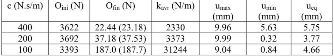
400 3622 22.44 (23.18) 2330 9.96 5.63 5.75

200 3692 37.18 (37.53) 3373 9.99 0.32 3.77

100 3393 187.0 (187.7) 31244 9.04 0.84 4.66

Table 2: Summary of the optimization analysis: step force F₀ =1200N.

equilibrium displacement. umax and umin are the maximum and minimum achieved in displacements, minimum value in displacement is considered after the first maximum peak.

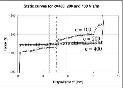
Figure 7: Final design of the static curves (detail of the plateau) with the equilibrium displacement designated by the vertical line, step force F₀ =1200N.

Several analyses were performed with different initial static curves. All analyses approximately gave the same values. It can be concluded, that the minimum value of the objective function and the plateau slope, increase with decreasing damping.

Reaction in initial and final design, c=400N.s/m

0 500 1000 1500 2000 2500 3000 3500 4000 4500

0 1 2 3 4

Time [s]

R

eact

io

n

[

N

]

Figure 8: Total reaction of the initial (dashed curve) and the optimized design (full curve) for c=400N.s/m.

Static curves for c=400, 200 and 100 N.s/m

900 1100 1300 1500

0 3 6 9 12

Displacement [mm]

For

c

e

[

N

]

200 c=

It is seen that the optimization procedure is very efficient if high c-values are considered. For low damping coefficient it was impossible to obtain a result, which would utilize the full plateau. In Figure 7 final static curves and in Figures 8 comparison of the total reaction of the initial and the optimized design is plotted for

N 1200

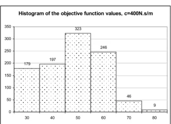
F₀ = . A sensitivity analysis of the obtained results was performed in the sense that objective function was calculated for 1000 design taken as the optimized static curve affected by one localized perturbation of one point within 1%. It is worthwhile to point out, that the ordering values procedure, rarely kept the perturbed value at the same place. As expected, the less optimized case (low c) showed the most stable values. In the following graphs of Figures 9-11, the histograms of the objective functions values are plotted, for the case of F₀ =1200N.

Histogram of the objective function values, c=400N.s/m

179

197

323

246

46 9 0

50 100 150 200 250 300 350

30 40 50 60 70 80

Figure 9: Histogram of the objective function values, c=400N.s/m.

Histogram of the objective function values, c=200N.s/m

18 19 25

46 126

399

279

78

0 50 100 150 200 250 300 350 400 450

50 80 110 140 170 200 230 260

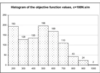
Histogram of the objective function values, c=100N.s/m

193

128 135 196

169

110

43 24

2 0

50 100 150 200 250

200 300 400 500 600 700 800 900 1000

Figure 11: Histogram of the objective function values, c=100N.s/m.

Next analysis confirms, that the perfect plateau is not an optimized design. Then internal bumps appear in the total reaction whenever the displacement value goes out from the allowable interval. It must be pointed out, that the first “design” point (0,0) is fixed and it corresponds to the static equilibrium position when no force is applied. This point is not included in the optimization procedure. Because 30 design values are used within 10mm interval, the first design point is located at 0.32mm. As a consequence, the allowable displacement interval is in fact only

(

0.32mm,10mm

)

. Results are summarized in Tables 3 and 4.

c (N.s/m) O (N) umax (mm) umin (mm) ueq (mm)

400 31.86 (31.90) 10.00 9.86 9.87

200 306.95 (307.04) 10.27 (bump) 0.32 0.50 100 938.59 (942.13) 10.40 (bump) 0.16 (bump) 0.51 Table 3: Summary of the results of the load case (i), step force F₀ =1000N, with the

static curve considered as the perfect plateau.

c (N.s/m) O (N) umax (mm) umin (mm) ueq (mm)

400 61.78 (62.00) 10.06 (bump) 9.03 9.03

200 458.77 (460.30) 10.33 (bump) 0.03 (bump) 2.28 100 1136.80 (1137.8) 10.46 (bump) 0.01 (bump) 4.20 Table 4: Summary of the results of the load case (i), step force F₀ =1200N, with the

static curve considered as the perfect plateau.

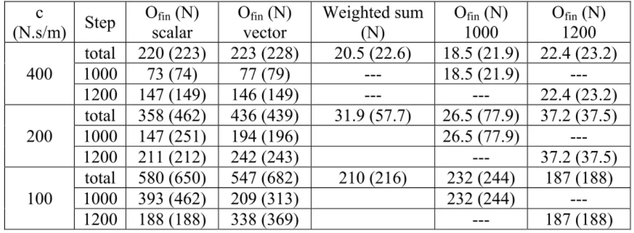
4.2 Load case (ii)

given by Equation (3). Results are summarized in Table 5. It is worthwhile to mention that now the optimization procedure can be run in two ways, cost functional can be assumed in its scalar value, or, optimization can require improvement in each Oi, i=1,2, to accept the corresponding design curve. This fact is designated in table as “scalar” and “vector” in the first row. No significant differences were found.

c

(N.s/m) Step

Ofin (N) scalar

Ofin (N) vector

Weighted sum (N)

Ofin (N) 1000

Ofin (N) 1200 400

total 220 (223) 223 (228) 20.5 (22.6) 18.5 (21.9) 22.4 (23.2) 1000 73 (74) 77 (79) --- 18.5 (21.9) --- 1200 147 (149) 146 (149) --- --- 22.4 (23.2) 200

total 358 (462) 436 (439) 31.9 (57.7) 26.5 (77.9) 37.2 (37.5) 1000 147 (251) 194 (196) 26.5 (77.9) ---

1200 211 (212) 242 (243) --- 37.2 (37.5)

100

total 580 (650) 547 (682) 210 (216) 232 (244) 187 (188)

1000 393 (462) 209 (313) 232 (244) ---

1200 188 (188) 338 (369) --- 187 (188)

Table 5: Summary of the optimization results of the load case (ii).

Optimised static curves are shown in Figure 12 for the scalar approach. It can be concluded, that formations of the respective plateaus at forces levels is not assured. Moreover, the difference between the optimization results from previous section is very large. Solution, which would mark plateaus at each equilibrium force level and within the range of corresponding displacements is impossible. In this formation there would be insufficient strain energy accumulated in the spring in order to prevent the bump at the maximum displacement. Therefore, mainly the higher plateau is above the second applied step force F_2,0 =1200N.

Static curves for c=400, 200 and 100 N.s/m

700 800 900 1000 1100 1200 1300 1400 1500 1600

0 3 6 9 12

Displacement [mm]

F

o

rce [

N

]

4.3 Load case (iii)

In this load case the objective function can take into account both regimes, the transient as well as the steady-state one. Nevertheless, and because the transient effect is only temporary, we started with weight parameters γ_tr =0 and γ_st =1. Then the optimization problem reduces to the minimization of transmissibility. In the linear case the transmissibility can be expressed as:

(

)

2

2 2

2 2 0

2 2 4

0

m c m

c

T

ω ⎟ ⎠ ⎞ ⎜ ⎝ ⎛ + ω − ω

ω ⎟ ⎠ ⎞ ⎜ ⎝ ⎛ + ω

= , (16)

where ω stands for the frequency of the excitation force and ω₀ for the natural frequency of the system. Usually, transmissibility is plotted with respect to the excitation frequency. But in our case, ω is fixed and spring rigidity (governing the natural frequency) is the design variable. Therefore the graph of transmissibility with respect to the natural frequency will indicate the expected optimization result. This graph is shown in Figure 13a) for f =50Hz and f =100Hz.

Figure 13: a) Transmissibility versus the natural frequency for excitation frequency

Hz 50

f = (full line) and f =100Hz (dashed line); b) Transmissibility versus excitation frequency according to Equation (9) for different values of c=100N.s/m

(full line), 200 N.s/m (dashed line) and 400 N.s/m (dotted line), respectively.

It is seen that the transmissibility achieves the lowest value when the natural frequency tends to zero. Therefore the optimised static curve will tend to a curve with a plateau at the equilibrium force, like in load case (i). Now the plateau can be

T

[ ]

Hz f₀

m / s N 200

c= ⋅

m / s N 400

c= ⋅

T

[ ]

Hz f

m / s N 100

developed only within the steady-state displacement range. Simplifying Equation (16) for ω₀ ≅0, one gets:

( )

2 2

C m

C T

+ ω

≅ , (17)

Then the graph of the transmissibility versus the excitation frequency for the different c-values used in this paper is presented in Figure 12b). It is seen from Figure 12b) that the transmissibility values are very low and that they increase with increasing damping. Low values of transmissibility will imply very low range of steady-state displacements and therefore hardly noticeable plateau. For this reason amplitude of the harmonic contribution was assumed as 500N instead of 1-2N. The optimised results confirmed all predictions. In each case plateau was easily formed and the objective function achieved the analytically lowest possible value. Results for excitation frequency ω=300rad/s=47.7Hz, F0=1000N and F1=500N are summarized in Table 6.

c (N.s/m) Oini (N) Ofin (N) Oanl (N) umax (mm) umin (mm)

400 212.77 25.84 (26.72) 26.66 7.54 7.32

200 100.57 13.01 (13.48) 13.33 7.08 6.85

100 102.26 6.84 (6.86) 6.67 8.03 7.79

Table 6: Summary of the optimization analysis for the load case (iii).

In Table 6 except for the values defined before, Oanl stands for the analytical value and umax and umin now refer only to the steady-state regime.

Static curves for c=400, 200 and 100N.s/m

800 850 900 950 1000 1050 1100 1150 1200

4 5 6 7 8 9 10

Displacement [mm]

For

ce

[

N

]

Figure 14: Final design of the static curves (detail of the plateau) with the range of steady-state displacements designated by two vertical lines, step force F0=1000N

Objective function is very stable in all these cases, because significant part of the static curve does not influence the total dynamic reaction in the steady-state regime. However, in all these cases there is a very high reaction peak in the transient part. Therefore, in the next analysis γ_tr =0.5 and γ_st =0.5 were assumed. As expected, optimized solution is now very similar to the one obtained in load case (i). Plateau is formed at the equilibrium force level, because this condition is required in both regimes. Part of the objective function corresponding to the steady-state regime again achieves the analytically lowest possible value. Results are summarized in Table 7, where also comparison with the previous results is given. Thus “Reg.” stands for the regime, which is separated into “total” (the total objective function) and the parts from the transition (“tr.”) and from the steady-state (“st.”) part. Third column summarizes the objective function values obtained in the current analysis. Fourth column shows the objective function value for load case (i) on optimized static curve from the current analysis; and the next column brings the current analysis objective function values on the optimized static curve from load case (i). Last two columns include, for the sake of comparison, final values from Tables 1 and 6 and sixth column designated “Sum” shows the weighted sum value if the optimum would be obtained in both regimes.

c

(N.s/m) Reg.

Ofin (N) comb.

O (N) step

O (N) comb.

Sum (N)

Ofin (N) step

Ofin (N) harmon. 400

total 33.4 (33.7) 62.39 32.4 22.2 18.5 (21.9) 25.8 (26.7)

tr 40.1 62.39 38.1 18.5 (21.9) ---

st 26.6 --- 26.7 --- 25.8 (26.7)

200

total 21.1 (21.3) 394 23.4 19.8 26.5 (77.9) 13.0 (13.5)

tr 28.9 394 33.5 26.5 (77.9) ---

st 13.3 --- 13.4 --- 13.0 (13.5)

100

total 65.1 (65.2) 756 138 119.4 232 (244) 6.8 (6.9)

tr 124 756 240 232 (244) ---

st 6.7 --- 37 --- 6.8 (6.9)

Table 7: Summary of the optimization analysis for the load case (iii).

Reaction comparison (c=400N.s/m)

800 900 1000 1100

0.2 0.4 0.6 0.8 1 1.2

Time [s]

R

eact

io

n

[

N

]

Figure 15: Reaction comparison related to Table 7, column 3 (full bold line), columns 4 (dotted line) and column 5 (full line), c=400N.s/m.

Reaction comparison (c=100N.s/m)

400 600 800 1000 1200

0.2 0.4 0.6 0.8 1 1.2

Time [s]

R

eact

io

n

[

N

]

Figure 16: Reaction comparison related to Table 7, column 3 (full bold line), columns 4 (dotted line) and column 5 (full line), c=100N.s/m.

4 Conclusions

development, especially in the design of new mechanical components such as engine mounts and /or suspension systems.

/Acknowledgements

The first author would like to thank to Fundação para a Ciência e a Tecnologia, of the Portuguese Ministry of Science and Technology for supporting expenses related to this congress (grant PTDC/EME-PME/67658/2006: “Design of cellular elastomeric materials for passive vibration control”).

References

[1] R.S. Lakes, “Extreme Damping in Composite Materials with a Negative Stiffness Phase”, Physical Review Letters, 86(13), pp. 2897-2900, 2001.

[2] R.S. Lakes, “High Damping Composite Materials: Effect of Structural Hierarchy”, Journal of Composite Materials, 36(3), pp. 287-297, 2002.

[3] Z. Hashin, “Viscoelastic Behavior of Heterogeneous Media”, Journal of Applied Mechanics, Trans. ASME, 32E, 630-636, 1965.

[4] M. Jirásek, Simple Non-linear System Simulation, Internal Report, Czech Technical University in Prague, 1988, (in Czech).

[5] I. Kovacic, M.J. Brennan, T.P. Waters, “A Study of a Nonlinear Vibration Isolator with a Quasi-Zero Stiffness Characteristics”, Journal of Sound and Vibrations, 315, pp.700-711, 2008.

[6] D.L. Platus, “Smoothing out Bad Vibes”, Machine Design, 26, pp. 123-130, 1993.

[7] T. Pritz, “Frequency Dependences of Complex Moduli and Complex Poisson’s Ratio of Real Solid Materials”, Journal of Sound and Vibrations, 214(1), pp. 83-104, 1998.

[8] J. Prasad, A.R. Diaz, “A Concept for a Material that Softens with Frequency”, Journal of Mechanical Design 130(9), 2008.

[9] D.I.G. Jones, “Handbook of Viscoelastic Vibration Damping”, J. Wiley &Sons, Ltd., 2001.

[10] Release R2007a Documentation for MATLAB, The MathWorks, Inc., 2007. [11] L. Meirovitch, "Elements of vibration analysis". McGraw-Hill, Kogakusha,

Ltd., 1975.