Design of New Materials for Passive Vibration Control

Abstract

The objective of this contribution is to extend the models of cellular/composite material design to nonlinear material behaviour and apply them for design of materials for passive vibration control. As a first step a computational tool allowing determination of optimised one-dimensional isolator behaviour was developed. This model can serve as a representation for idealised macroscopic behaviour. Optimal isolator behaviour to a given set of loads is obtained by generic probabilistic meta-algorithm, simulated annealing. Cost functional involves minimization of maximum response amplitude in a set of predefined time intervals and maximization of total energy absorbed in the first loop. Dependence of the global optimum on several combinations of leading parameters of the simulated annealing procedure, like neighbourhood definition and annealing schedule, is also studied and analyzed. Obtained results facilitate the design of elastomeric cellular materials with improved behaviour in terms of dynamic stiffness for passive vibration control.

Keywords: cellular materials design, passive vibration control, non-linear

visco-elastic behaviour, optimization, simulated annealing, cost functional.

1 Introduction

Contribution of computational mechanics has been essential in the more recent and remarkable developments on structural design and optimization. Now the same impact and influence can be predicted in its application for new materials design, within the framework of micromechanics. The latest developments in these areas have lead to integrated computational methodologies that permit not only the structural design of the mechanical component but also the design of the material used in its fabrication. This is particularly evident in the area of cellular/composite materials where the unit cell geometry (characterizing the composite or cellular

Design of New Materials for

Passive Vibration Control

T. Lopes1, Z. Dimitrovová1, L. Faria2and H.C. Rodrigues2

1_{Department of Civil Engineering}

UNIC, New University of Lisbon, Portugal

2Department of Mechanical Engineering

IDMEC/IST, Technical University of Lisbon, Portugal

in B.H.V. Topping, M. Papadrakakis, ( Edit ors) , " Proceedings of t he Nint h

material) is a key factor in its effective mechanical properties and thus can significantly improve the structural response of the mechanical component.

The objective of this contribution is to extend the models of cellular/composite material design to nonlinear material behaviour and apply them for design of materials for passive vibration control. First of all a computational tool allowing determination of optimised one-dimensional isolator behaviour was developed. Such behaviour can be used as a model for idealized one-directional macroscopic behaviour. Then multi-direction optimal properties must be stated according to the problem under consideration. Obtained results can be used as target behaviour for subsequent cellular/composite material design.

In this contribution optimal isolator behaviour to a given set of loads is obtained by generic probabilistic meta-algorithm, simulated annealing. In order to characterize non-linear elastic behaviour, fixed parts of the static curve were identified and variable parts were estimated by piece-wise cubic hermit polynomial expressions with flexible number of divisions and random target forces. The algorithm assures positive stiffness at any instant, in order to avoid unstable behaviour. Damping is assessed by a linear viscous contribution. Cost functional involves minimization of maximum response amplitude in a set of predefined time intervals and maximization of total energy absorbed in the first loop, later feature is still under development. Dependence of the global optimum on several combinations of leading parameters of the simulated annealing procedure, like neighbourhood definition and annealing schedule, is also studied and analyzed. Most computational tools are developed in numerical computation software Matlab [1], some results were confirmed in symbolical and numerical computation software Maple [2] and general purpose finite element software ANSYS [3].

Paper is organized as follows. In Section 2 problem statement is given. Firstly, assumptions and simplifications are summarized in order to define optimization problem for one-dimensional isolator behaviour. Then procedures required for non-linear behaviour definition are described in more details. Section 3 is dedicated to optimization algorithm description and Section 4 presents obtained results. Paper conclusions are summarized in Section 5.

Presented results, although still related only to one-dimensional behaviour, facilitate the design of elastomeric cellular/composite materials with improved behaviour in terms of dynamic stiffness for passive vibration control. Future research will be directed to optimization of multidirectional properties, which will be used as target behaviour for design of cellular and/or composite viscoelastic materials. This application will have a direct and immediate impact on product design and development, especially in the design of new mechanical components such as engine mounts and /or new suspension systems.

2.1 Optimal one-dimensional behaviour

It is assumed that mass of a given value, m, is connected through isolator, s(t), to fixed support. Mass is exited by time dependent set of forces, P(t). The objective is to determine isolator characteristics which will provide an optimal dynamic response of the system. Reaction exhibited by the support, R(t), is selected as a crucial result for optimization according to practical applications (see Figure 1). Maximum amplitude of the reaction R(t) is intent to be minimized in the transient as well as in the steady-state part of the time dependent response. Usually such requirement is implemented in an absolute sense in the transient part, i.e. when the natural vibration contribution is still present. In the steady-state part of the response this condition can be substituted by minimization of transmissibility, thus in this case optimization can be thought in a relative sense as minimization of the ratio of the reaction amplitude over the excitation harmonic force amplitude.

Figure 1: Problem scheme.

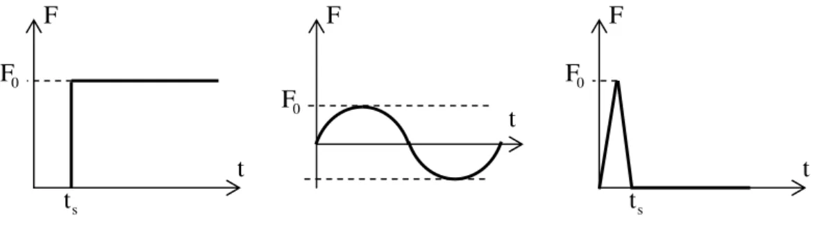
First of all it is necessary to state, what kind of excitation forces are included in the analysis. Load cases are chosen according to the practical applications as: (i) step load, (ii) step load, where probability of the step force follows normal distribution with given value of standard deviation, (iii) harmonic load, (iv) set of harmonic loads, (v) impact load, (vi) impact load, where probability of the impact force follows normal distribution with given value of standard deviation, (vii) combination of previous cases. Load cases (i), (iii) and (v) are schematically represented in Figure 2.

Figure 2: Schematic representation of load cases (i), (iii) and (v). F

0 F

t s

t

F

0 F

t

F

0 F

t s

t m

( )

t s

( )

t P

( )

t

u m

( )

t s

( )

t P

( )

t u

Next, it is necessary to make some assumptions about the isolator behaviour. In the initial stage of this study, nonlinear elastic and linear visco-elastic behaviour is assumed. Therefore the isolator can be schematically substituted as indicated in Figure 3.

Figure 3: Schematic representation of the isolator.

In Figure 3, k

( )

u

( )

t stands for the rigidity of the nonlinear spring and c is the damping constant of the linear damper and “dot” as usual represents time derivative. Damping constant c in this case affects only the value of “transition” time, t_r, as the time which separates the transient and the steady-state region in the time dependent response, i.e. upto which contribution of natural vibrations cannot be omitted. In such specification damping constant is not subject of optimization. Equation of motion of the system from Figure 3 is, [4]:

( )

t cu

( )

t k

( ) ( ) ( )

u

( )

t u t P t mg u

m&& + & + = + , (1)

where g is acceleration of gravity. The support reaction is given by

( )

t cu

( )

t k

( ) ( )

u

( )

t u t

R = & + . (2)

Optimization problem for the load cases (ii), (iii) and (vi), specified in Figure 2, can be stated as

find k

( )

u

( )

t , such that

( ) ( ) ⎟⎟_⎠ ⎞ ⎜⎜ ⎝ ⎛ γ + γ = ∈ ∈ ∈ f r r

i t t;t

st st t ; t t tr tr S t u k

0 min A A

O , (3)

where A and _tr A stand for the maximum amplitude of the support reaction in the _st transient and in the steady-state region, respectively; t_i and t_f correspond to the initial time (from where the transient response gains importance), and to the final time of the analysis, respectively. In more detail:

( )

t min R

( )

t R max A r i r

i;t t t;t

t t

tr = _∈ − _∈ and A max R

( )

t min R

( )

t

f r f

r;t t t;t

t t

st = _∈ − _∈ , (4)

m

( )

t P

( )

t u

( )

t u c&

Further in Equation (3), γ_tr and γ_st are convenient weights, highlighting the relative importance of each regime and with the property γ_tr +γ_st =1, subscript “0” in objective function O means that in load cases (i), (iii) and (v) only “single” force ₀ characterized by F is involved, see Figure 2. Obviously for step load (i) ₀ t_i>t_s and

0 st =

γ ; for harmonic load (iii) t_i=0 and both weights can be non-zero; for impact load (v) t_i =0 and γ_st =0. As expected, the second part of the objective function

0

O is important only for harmonic loads (iii). Then A can be substituted by _st transmissibility T, as explained in the beginning of this section, T=A_st/

( )

2F₀ . If

0

O combines absolute and relative criterion, special attention must be paid to γ_tr and γ_st selection.

Load cases (ii) and (vi) can be simplified by a set of discrete cases, where weights i

λ can be calculated according to the normal distribution of F with given standard ₀ deviation. Cost functional O is then defined as:

∑

− =

λ

= s

s i

i i

i O

min

O , (5)

where 2s+1 stands for the number of selected discrete cases, including F with the ₀ maximum probability. Load case (iv) uses the same optimization statement as in Equation (3), but weights λ_i are fixed and conveniently chosen. Sum in this case is performed from 1 to n, where n is the number of harmonic loads. Combination of previous load cases (case (vii)) requires careful analysis of the corresponding weights in order to capture normalize contribution of each constituent part.

2.2 Optimization of nonlinear spring

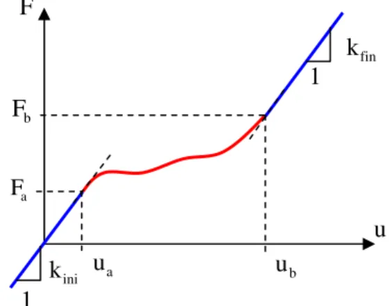
Let us concern with the nonlinear spring definition, which will allow us to establish the rules for optimization. In order to characterize nonlinear elastic behaviour, fixed and variable parts of the static curve must be identified. Practical applications require that spring rigidity is not arbitrary. There is an initial and a final linear stage characterized by initial and final rigidity, as shown in Figure 4. Further, F stands _a for the given mass weight (mg) and u is the corresponding static displacement. _a Final part is restricted by rigid component, which starts to actuate when the maximum allowable displacement u of the flexible part is achieved. Variable (red) _b part of the static curve in Figure 4 is the subject of optimization. It must be estimated by a convenient curve satisfying certain requirements in the full interval

b a,u

u :

b) Static curve must be strictly increasing, i.e. stiffness must be positive at any instant, in order to avoid unstable behaviour. This assumption can be violated at isolated points.

c) Static curve should have first derivative continuous, i.e. stiffness should be continuous at any instant. This assumption can also be violated at isolated points.

Figure 4: Nonlinear spring: fixed (blue) and variable (red) parts of the static curve. In order to determine the optimal static curve shape an optimization procedure must be implemented. In our case generic probabilistic meta-algorithm, simulated annealing, was chosen for this purpose. The algorithm will be described in the next section. In addition to the cost functional, defined in Equations (3-5), and simulated annealing general steps, several procedures must be established. For instance a well-defined procedure for variable part of the static curve definition must be given. Then it is possible to solve the problem stated in Equation (1) numerically using predefined numerical integration algorithm, incorporated in Matlab software, calculate the reaction according to Equation (2) and evaluate the cost function for such particular case. One of the possible approaches for the static curve definition is: a) select a set of fixed points ui,i=1,...,n ordered increasingly from the given

open interval

(

u_a,u_b

)

;

b) Randomly select force values F_i,i=1,...,n from the given open interval

(

Fa,Fb

)

, order them in an increasing way and attribute them to the selected

points ui;

c) Define spline approximation within each interval u_a,u₁ ,

1 n ,..., 1 i , u ,

u_{i i+1} = − and u_n,u_b .

Let u_a =u₀, u_b =u_n+1, F_a =F₀ and F_b =F_n+1. Regarding a), without restricting the generality, uniform distribution of interval u_a,u_b can be assumed, thus

n ,..., 0 i , u u n

u u

u= n 1− 0 = _i1− _i ∀ =

Δ + _{+ . As far as the spline approximation, linear and} fin

k 1

ini

k ua

1

b

u

u

b

F

a

F

cubic Hermite approximations were tested for suitability. Linear spline approximation is easy to implement, it preserves continues and monotonic behaviour, however it violates requirement c).

Cubic Hermite approximation, on the other hand, establishes cubic polynomial approximation within each interval with continuity of the first derivative in the separation points u_i. Then the initial and the final derivative at u and _a u can _b correspond to k_ini and k_fin, as indicated in Figure 4. Let k_ini =d₀ and k_fin =d_n+1. Derivatives at the intermediate points u_i,i=1,...,n can be given by finite differences, as forward, backward or centred approximation. Implementation of Hermite approximation is also straightforward, requirements a) and c) are assured, however, requirement b), is not preserved.

Monotonic behaviour is a crucial condition, therefore some adjustments must be implemented. Following [5], if the conditions for monotonicity are not met in a certain interval, derivatives at the end points of this interval, d_i and d_i+1, should be corrected to τd_i and τd_i+1, where

2 2

3

β + α =

τ , (6)

and

δ = α di _,

δ =

β di+1 _and

u F F_{i 1 i}

Δ − =

δ + _{. (7)}

Note that in our case k_ini and k_fin are fixed. To handle this limitation, we set 1

=

β and α=1 at the first and in the last interval, respectively. Then, if random forces are selected from

(

F_a+d_iniΔu/4,F_b−d_finΔu/4

)

, instead of

(

F_a,F_b

)

, all monotonicity conditions are fulfilled in these intervals and no alteration of k_ini and

fin

k is required.

Figure 5 shows one possible choice of random forces, which is already related to the case study described further in this paper. Random values are connected by linear spline, red points mark initial end-points intervals, where at least one of the monotonicity conditions is not satisfied.

0 500 1000 1500 2000 2500

0.005 0.007 0.009 0.011 0.013 0.015

Displacement [m]

For

ce [

N

]

Figure 5: A possible choice of random forces. Red points identify the initial point of each interval where monotonicity conditions are not satisfied.

977 978 979 980 981 982

0.0064 0.0066 0.0068 0.0070

Displacement [m]

For

ce [

N

]

Figure 6: Efficiency of the monotonicity criteria: Hermite approximation before (blue) and after (red) derivatives alteration.

3 Optimization algorithm

As already mentioned, generic probabilistic meta-algorithm, simulated annealing, was chosen as optimization tool to solve the problem specified in Equation (3-5). For this let us assume that at iteration k one has the respective static curve and objective function value O_k. Then for the next iteration (k+1) we create a new static curve in the “neighbourhood” of the old one and compute the new objective function value O_k+1. If O_k+1<O_k then the new static curve is unconditionally accepted. If

k 1

k O

O ₊ ≥ then it is conditionally accepted based on the probability calculated as

(

)

(

O O /T

)

exp _k − _k+1 , when T is the current cooling temperature. This criterion prevents the algorithm to stick at local minimum and gives the possibility to search through the entire design domain. As the cooling proceeds, i.e. T is gets lower and consequently the probability of acceptance decreases. Nevertheless global optimum is never guaranteed and usually several attempts must be performed in order to obtain reliable results.

There are several crucial parameters in this algorithm which must be carefully chosen as they can distort the final result and/or make the calculation inefficient. They are:

a) initial temperature,

b) number of iterations within each temperature, c) cooling schedule,

d) stopping criteria,

e) neighbourhood definition.

Initial temperature is usually defined as a ratio of the initial value of the cost functional. It should be stated in the way that acceptance probability in the initial temperature stage is around 50%. Number of iterations within each temperature must be high, around 500 or more and must be adapted to each particular load case. It does note make much sense to implement many temperature levels, since then probabilities in two consequent temperatures will be very similar. Note that the algorithm can stop before completing the cooling schedule, whenever the number of consecutive failures reaches the user-input number.

Neighbourhood definition is crucial in a simulated annealing algorithm. In our problem it is defined in percentage terms from the given static curve. In more details, user-input values are:

a) m≤n as number of forces which are allowed to vary; b) p the percentage of variation.

After the new force values are obtained they must be ordered in an increasing way, in order to satisfy requirements specified in Section 2.2.

4 Obtained results

Engine mount suspension system is assumed as a practical application. Then F in ₀ load cases (i-ii) and (v-vi) have relatively high values, around 1000-2000N, while

0

F in load case (iii) are around 1-2N with frequencies from 25Hz to 250Hz. The former case represents the action exerted on engine in acceleration or sudden car stop. Harmonic forces are exerted on engine in idling regime, i.e. when the engine runs without car movement. Harmonic forces are generally always superposed to the other step or impact load, whenever the engine is running. This means that load cases (i-ii), (v-vi) cannot occur in real applications, nevertheless they are worthwhile study individually to draw conclusions about their particular effect.

Further data are: mass m=50kg, yielding u₁ =5mm and k_ini ≅100N/mm. Final part of the static curve from Figure 4 is then limited by the maximum admissible displacement of the flexible part of the support, u₂ =15mm. After that rigid components of the support start to actuate, thus obeys linear behaviour of rigidity around k_ini ≅1000N/mm. Damping is set at c=408.046kg/s.

4.1 Load case (i)

Besides other values defined in previous sections, this load case is characterized by N

1200

F₀ = , st_s =0.3 and t_fin =0.3s. According to Equations (3-4) the objective function is characterized by γ_tr =1, 0γ_st = and t_i>t_s. The static curve has n=20 force values and the neighbourhood is defined by m=10 and p=15%.

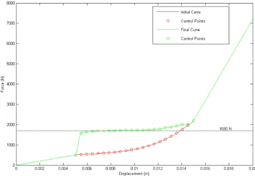
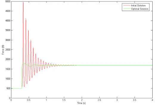
Several analyses were performed with different initial static curves. All solutions indicate that the optimal static curve has a “plateau” at the force level F₀+mg, as it is shown in Figure 7. Figure 8 shows initial and optimised system response. It is seen that the optimised response is almost completely smoothed on the maximum force level F₀+mg.

Figure 8: Initial (red) and optimised (green) system response in load case (i).

4.2 Load case (ii)

Here we assumed that the applied load can vary between lower and upper bounds. For simplicity we considered only three forces F₋₁=1000N, NF₀ =1200 and

N 1400

F₁= with occurrence probability characterized by load factors λ_i,i=−1,0,1.

Optimised results for two cases are presented in Figures 9-10. The first one corresponds to λ₋₁=0.25, 5λ₀ =0. and λ₁ =0.25 and the second one to λ₋₁=0.5,

25 . 0 0 =

Figure 7: Initial (red) and optimised (green) static curve in load case (ii) with

N 800

F₋₁= , NF₀ =1000 , F₁ =1200N and λ₋₁=0.25, 5λ₀ =0. , λ₁=0.25.

Figure 10: Initial (red) and optimised (green) static curve in load case (ii) with

N 800

F₋₁= , NF₀ =1000 , F₁ =1200N and λ₋₁=0.5, 25λ₀ =0. , λ₁=0.25.

In this load case the objective function is characterized by γ_tr =0 and γ_st =1 thus transmissibility is optimised. In the linear case transmissibility can be expressed as:

(

)

2

2 2

2 2 0

2 2 4

0

m c m

c

T

ω ⎟ ⎠ ⎞ ⎜ ⎝ ⎛ + ω − ω

ω ⎟ ⎠ ⎞ ⎜ ⎝ ⎛ + ω

= , (8)

where ω stands for the frequency of the excitation force and ω₀ for the natural frequency of the system. Usually transmissibility is plotted with respect to force frequency. In our case the objective is different, because ω is fixed and rigidity is the design variable. The plot of transmissibility with respect to the natural frequency will suggest the expected optimization result. For f =50Hz and f =200Hz this plot is shown in Figures 11 and 12, respectively. It is seen that the optimised curve will tend to a static curve with plateau at the equilibrium force level, like in previous cases. In order to prevent formation of plateau at zero force level, which is not possible due to problem statement definition, a constant force is added to the harmonic one.

Figure 11: Transmissibility versus natural frequency for excitation force frequency

Hz 50 f =

T

Figure 12: Transmissibility versus natural frequency for excitation force frequency

Hz 200 f =

Figure 13: Transmissibility according to Equation (9) for different values of c=204.023kg/s, 408.046kg/s and 612.069kg/s, respectively.

Simplifying Equation (9) for ω₀ ≅0:

( )

2 2 C m

C T

+ ω

≅ , (9)

yielding T=0.025 and 0.0065 for f=50Hz and f=200Hz, respectively. These values were verified by the optimised results. Moreover, on the contrary to the statement in

s / kg 023 . 204 c=

s / kg 046 . 408 c=

s / kg 069 . 612 c= T

s / rad

T

Section 2, now c plays an important role. Figure 13 shows the variation of transmissibility according to Equation (9) for different values of c=204.023kg/s, 408.046kg/s and 612.069kg/s, respectively.

5 Conclusions

The work described here is a first step to design materials for passive vibration control. From the results obtained it is apparent that optimal behaviour can be achieved, however it is also clear that a precise definition of existing forces and design constraints is crucial for its success in practical applications. Once the optimal static curve(s) is identified future research will be directed to the design of cellular and/or composite viscoelastic materials achieving this behaviour(s). This application will have a direct and immediate impact on product design and development, especially in the design of new mechanical components such as engine mounts and /or suspension systems.

References

[1] Release R2007a Documentation for MATLAB, The MathWorks, Inc., 2007. [2] Release 11 Documentation for Maple, Maplesoft a division of Waterloo

Maple, Inc., 2007.

[3] Release 11.0 Documentation for ANSYS, Swanson Analysis Systems IP, Inc., 2007.

[4] L. Meirovitch, "Elements of vibration analysis". McGraw-Hill, Kogakusha, Ltd., 1975.