Quadrotor Simulator for Control De- velopment – Application to Autono- mous Landing

(1)

Ricardo dos Santos Moreira

Licenciado em Ciências da Engenharia Electrotécnica e de Computadores

Quadrotor Simulator for Control

De-velopment

–

Application to

Autono-mous Landing

Dissertação para Obtenção do Grau de Mestre em Engenharia Electrotécnica e de Computadores

Orientador: Professor Doutor Fernando Coito, Professor Au-xiliar, FCT-UNL

Júri

Presidente: [Nome do orientador], [Cargo], [Instituição] Arguentes: [Nome do co-orientador 1], [Cargo],

[Institui-ção]

(2)

(3)

Quadrotor Simulator for Control Development – Application to Autonomous Landing

(4)

(5)

(6)

(7)

Acknowledgments

In the first place, I would like to thank my advisor, Professor Doctor Fer-nando Coito, for the guidance and patience when silly questions were asked. The knowledge I gain from this work and from his advices are certainly going to help me as an engineer. For that, I thank you.

Thanks to Vasco Brito for helping me to understand some of his work, which contributed to the development of this thesis.

For the best persons I know, a deeply thanks and acknowledgment for my parents, who always gave me support and stood beside me in the good and bad moments. Without them, I would not be where I am now.

(8)

(9)

Abstract

In this thesis is studied the landing problem of a VTOL UAV and a 3D sim-ulation environment is built to safely develop control for a quadrotor, resorting to 3D modelling and simulation software.

In a time where the development of unmanned vehicles is a trend and it is technologically in growth, the emergent difficulties are challenging when it comes to aviation. In this field, it is useful a tool for researchers to have at their disposal to conduct experiments without putting their real systems to real threat. Also, the landing of UAV’s is currently one of the most serious cases of study with a lot of investigation going on to solve the problems associated with it. In this sense, some problematics are contemplated.

Based on a quadrotor in a X8 configuration – 4 frames and 8 propellers –, are applied linear and nonlinear control design techniques with the intent to sta-bilize and control the quadrotor and a 3D simulator is developed.

Keywords: 3D simulation; landing considerations; quadrotor; unmanned

(10)

(11)

Resumo

São abordados, nesta tese, alguns problemas associados com a aterragem de um veículo do tipo VTOL UAV. Em adição, um ambiente de simulação 3D é construído com o intento de, em segurança, desenvolver controlo a aplicar em quadrotores, recorrendo, assim, a ambientes de modelação e simulação 3D.

Numa época em que o desenvolvimento de veículos não-tripulados é uma tendência e está tecnologicamente em crescimento, as dificuldades emergentes são desafiantes no que concerne à aviação. Nesta área, é como uma mais-valia uma ferramenta ao alcance de investigadores, de forma a que estes possam con-duzir as suas experiências sem colocar em risco qualquer instalação física. Em adição, a aterragem de veículos aéreos não-tripulados apresenta-se como um sé-rio caso de estudo, existindo, ainda, bastante investigação a ser conduzida de forma a resolver os problemas associados à mesma. Neste sentido, algumas pro-blemáticas são contempladas.

Baseado num quadrotor em configuração X8 – 4 braços e 8 hélices –, são aplicadas técnicas de controlo linear e não-linear com o intento de estabilizar e controlar o quadrotor. Em adição, um simulador 3D é desenvolvido.

Palavras-chave: simulação 3D; aterragem; quadrotor; veículo aéreo

(12)

(13)

Nomenclature

Acronyms

2D – Plane representation 3D – Space representation

BLDC – Brushless Direct Current CPU – Central Processing Unit GE – Ground Effect

IGE – In Ground Effect

IMU – Inertial Measurement Unit OGE – Out of Ground Effect PD – Proportional-Derivative PI – Proportional-Integral

(14)

TF – Transfer Function

UAV – Unmanned Aircraft Vehicle VTOL – Vertical Take-off and Landing

Symbols

Symbol Description Unit

Cd drag coefficient adimensional

Cl lift coefficient adimensional

F, f force N

g gravity m.s-2

h height m

I body inertia kg.m2

k discrete-time variable samples.s-1

L, l length m

M total body mass kg

r radius m

t continuous-time variable s

T thrust N

Tτ torque induced by thrust N.m

TPWM PWM period s

𝑥, 𝑦, 𝑧 translational position m

𝜙, 𝜃, 𝜓 Euler angles rad

(15)

𝑝, 𝑞, 𝑟 body axes rate rad.s-1

τ Torque N.m

v linear speed m.s-1

(16)

List of Tables

Table 3.1: Roll / pitch controllers’ gains obtained via PSO method. ... 58

Table 3.2: Controllers’ gains obtained via Ultimate Sensitivity method. ... 59

Table 3.3: Attitude controllers’ gains obtained via PSO method. ... 62

Table 3.4: Altitude controllers’ gains obtained via Ultimate Sensitivity method.

... 63

Table 3.5: Position controllers’ gains obtained via Ultimate Sensitivity method.

(20)

(21)

List of Figures

Figure 2.1: Vasco Brito’s quadrotor. Retrieved from (Brito 2016). ... 31

Figure 2.2: Quadrotor and moving target (Lee, Ryan, and Kim 2012). ... 39

Figure 2.3: Quadrotor used for experimental results (Herissé et al. 2012). ... 40

Figure 2.4: Quadrotor used in experimental setup (Serra et al. 2016) ... 41

Figure 3.1: Representation of the quadrotor steady hovering. XYZ axes are represented by RGB arrows, respectively. Retrieved from (Brito 2016). ... 43

Figure 3.2: One-rotor configuration. ... 52

Figure 3.3: Two-rotor configuration... 52

Figure 3.4: PWM and Force signals conditioning. ... 55

Figure 3.5: Step response to pitch / roll speed closed-loop system. Controller’s gains based on PSO method. ... 58

Figure 3.6: Marginally stable ascension speed closed-loop system. ... 60

Figure 3.7: Step response to ascension speed closed-loop system. Controller’s gains based on Ultimate Sensitivity method. ... 60

Figure 3.8: Attitude control scheme. ... 61

Figure 3.9: Altitude control scheme. ... 62

Figure 3.10: Position control scheme... 63

Figure 3.11: Back-calculation Anti-Windup with PID controller. ... 65

(22)

Figure 4.2: Rotation response to a variable pitch setpoint. From left to right, body and Euler angles... 69 Figure 4.3: Control actions in response to pitch error. From left to right, altitude

and pitch control actions. ... 70 Figure 4.4: Control actions in response to pitch error. From left to right, force to

be applied by each rotor and pitch control action. ... 70 Figure 4.5: Rotation response to a variable yaw setpoint. From left to right, body

and Euler angles. ... 71 Figure 4.6: Control actions in response to yaw error. From left to right, altitude

and yaw control actions. ... 72 Figure 4.7: Rotation response to a step input signal applied to roll and pitch.

From left to right, body and Euler angles. ... 73 Figure 4.8: Control actions in response to roll and pitch error. From left to right, altitude and attitude control actions. ... 73 Figure 4.9: Rotation response to a step input signal applied to pitch and yaw.

From left to right, body and Euler angles. ... 74 Figure 4.10: Control actions in response to pitch and yaw error. From left to

right, altitude and attitude control actions. ... 75 Figure 4.11: Rotation response to a step input signal applied to roll, pitch and

yaw. From left to right, body and Euler angles. ... 76 Figure 4.12: Control actions in response to roll, pitch and yaw error. From left to

right, altitude and attitude control actions. ... 76 Figure 4.13: Translational response to a variable altitude setpoint. ... 77 Figure 4.14: Control action in response to altitude error. ... 77 Figure 4.15: Translational response to a variable setpoint applied to X axis. ... 78 Figure 4.16: Control actions in response to X error. From left to right, altitude

and pitch control actions. ... 79 Figure 4.17: Translational response to a step input signal applied to X and Y

axes... 80 Figure 4.18: Control actions in response to X and Y error. From left to right,

(23)

Figure 4.19: Translational response to a step input signal applied to X, Y and Z axes... 81 Figure 4.20: Control actions in response to X, Y and Z error. From left to right,

altitude and attitude control actions. ... 82 Figure 4.21: Thrust ratio at zero air speed and constant power. ... 83 Figure 4.22: Thrust ratio at forward speed and constant power. ... 83 Figure 4.23: Fall, touchdown and rebound: Altitude variation, reaction to

impact and control action 𝑈1. ... 84 Figure 4.24: Fall, touchdown and rebound: rest... 85 Figure 4.25: Translational response to a variable altitude setpoint. Air drag is

considered. ... 86 Figure 4.26: Control action in response to altitude error. Air drag is considered.

... 87 Figure 4.27: Translational response to a variable setpoint applied to X axis. Air

drag is considered. ... 88 Figure 4.28: Control actions in response to X error. From left to right, altitude

and pitch control actions. Air drag is considered. ... 88 Figure 4.29: Translational response to a step input signal applied to X, Y and Z

axes. Air drag is considered. ... 89 Figure 4.30: Control actions in response to X, Y and Z error. From left to right,

altitude and attitude control actions. Air drag is considered. ... 89 Figure 4.31: Fall, touchdown and rebound: Altitude variation, reaction to

impact and control action 𝑈1. Air drag is considered... 90 Figure 5.1: Quadrotor 3D model assembled in Blender. ... 93 Figure 5.2: Example of Blender v2.78 workspace. ... 94 Figure 5.3: Quadrotor physics assembly. Collision detection and other physics

considerations are embodied for simulation. ... 95 Figure 5.4: Project inputs. Definition of the input commands and the hardware

from which they are sent. ... 96 Figure 5.5: Set linear speed function on the constructor graph. Event graph has

(24)

Figure 5.6: Game viewport. The quadrotor 3D model and the scene are

represented. ... 97 Figure 5.7: Input process flow. From the player actuation to the resultant game

(25)

1 Introduction

1.1 Motivation

One of the main reasons why technology has accomplished many and great deeds has to do with wars. Every challenge that stepped in the way of science, were keenly overcame in order for groups of individuals to compete and surpass their foes. Or, in other words, to do harm. Nowadays, and fortunately, the thoughts are settled elsewhere. People are encouraged to thrive so others can benefit from the results and learn more about the planet and universe we live in. And even if the results are not that appealing, at least a piece of knowledge can be extracted and can motivate others to do better.

(26)

in complete autonomy. These are called UAV and are most likely the future of private and commercial flights.

The UAV’s are currently used for scouting, mapping, leisure, professional

photography and others, but can have a key role in the near future, as such in rescue missions, environmental monitoring, terrain analysis, infrastructures in-spection, and much more.

Despite some important achievements concerning attitude and trajectory control, the landing control is still an issue and is one of the most vital systems in an UAV. Also, to prevent any type of accidents, which can be disastrous, a 3D simulation environment for a quadrotor is developed, which is the main contri-bution of this work.

1.2 Research objective and main contributions

This research purpose is to discuss the landing problems of UAV’s and

de-velop a 3D simulation environment where this and other flight problems may be tested in safety.

The main goal of this thesis is to design a simulation environment with the intent to perform several tests concerning the landing of a UAV. For this purpose, a kinematics model of the aircraft has to be considered. As such, a specific quad-rotor is studied and controllers are developed on Matlab software, with the re-spective results presented at Chapter 4. The simulator will only include the quad-rotor model, but it will be possible to manually control it, with the prospective to receive the input commands from an external controller or one to be built-in.

(27)

the designed controllers are able to provide the necessary stability and perfor-mance to execute a successful flight.

1.3 Thesis Structure

This thesis is structured in 6 chapters, which are organized as follows: Introduction: In this chapter, are presented the motivation, the objectives and the main contributions to unmanned aviation. Also, the thesis structure is described.

State of the Art: In this chapter, the most relevant background information that supports this thesis is provided. Are referred the landing problems, the quadrotor for which the control is to be developed, an analysis on computer graphics software, control design techniques and finally the related work.

Quadrotor Dynamics and Control: Here is presented the quadrotor model used as starting point for this project, followed by improvements for a better nav-igation. Additionally, each motor TF is considered, problems associated with landing are considered and, to complete this chapter, are designed the controllers to be implemented on the closed-loop system.

Simulation and Results: This chapter intent is to validate the efficiency of the control architecture in the proposed model. Also, tests are conducted on cer-tain physics aspects to understand their influence in a real landing manoeuvre.

(28)

(29)

2 State of the Art

2.1 Introduction

In this chapter, it is presented the literature and scientific surveys of the areas of study used as milestones for this work. A briefly insight into some main problems in the aeronautics field is given, as well as their influence on landing phase of flight.

Following the problems associated with landing, the quadrotor kinematics model in which this thesis is grounded is presented. This model is a simplified version and does not considers several physics phenomena that has impact on landing approach.

(30)

Afterwards, are specified the techniques to be applied, so a satisfactory con-trol over the aircraft can be provided. The main steps to land a VTOL are to ac-quire the target, stabilize the aircraft, analyse the target surface and execute the right control actions for a perfect landing.

To end this chapter, it is presented the ground work for this thesis consti-tuted by a few researches conducted in past recent years.

2.2 The Landing Conundrum

Many are the effects that can cause a quadrotor to experience some difficul-ties. Since the first flight attempts that inventors and researchers are trying to nullify these. The most relevant ones are explained below.

2.2.1 Weather effect

Weather plays a significant role in every step of an aircraft navigation, from take-off to landing. For instance, changes in temperature lead to a variation of air density, which in turn leads to changes of air pressure. Ultimately, due to these events, air currents are formed. Altitude is also relevant, because the higher the aircraft, lesser the pressure and thinner the air, causing the aircraft to experience stability issues. These phenomena alters both the stall speed and minimum flying speed necessary for any aircraft to take-off or land, respectively (Federal Aviation Administration 2016).

Air flows, also known as winds, can interfere greatly on flight control. It can be a major setback on the quadrotor normal operation mode, because not only the quadrotor tends to deviate in a randomly way, but without a sufficiently ro-bust controller it might crash.

(31)

atmospheric pressure, the Coriolis effect and even the topography. As a result, it is of an utmost difficulty to write down a mathematical notation to characterize this phenomenon. However, the impact of it over an object can be measured. A way to represent this is through eq. (2.2.1) and eq. (2.2.2).

𝐹 = 𝑃 ∙ 𝐴 ∙ 𝐶𝑑 (2.2.1)

𝐹 =1₂∙ 𝜌 ∙ 𝑉2_{∙ 𝐴 ∙ 𝐶}

𝑑 (2.2.2)

Where 𝐹 is the drag force, or wind load, 𝑃 [Pa] is the wind pressure, 𝐴 [m2_] is the area section of the object where the force is being exerted, ρ [kg∙m-3_{] is the} air density, 𝑉 [m∙s-1_{] is the speed of the body relative to the air flow and}𝐶

𝑑 is the

drag coefficient.

2.2.2 Effect of Obstructions on Wind

As denoted in the previous subsection, wind is very unpredictable in each time instant, if taking solely into account natural causes. This condition might be

aggravated if structures are near and on wind’s side, wherein forms more turbu-lence and the changes of wind direction become even more random.

(32)

2.2.3 Ground Effect

When a VTOL aircraft is about to land, it experiences some undesirable phe-nomena due to ground effect. This happens when the air mass generated by the rotor blades is reflected by the surface, thus creating an air cushion, which is an air pressure on the lower side of the aircraft. This airflow can provide more thrust, leading to an increase of efficiency of the rotors. The main consequences of this principle includes vibration, which can lead to irreversible instability of the aircraft, altitude fluctuations (Davis and Pounds 2016; Sharf et al. 2014; Aich et al. 2014), and possible bounce after touching a rigid surface (ArduPilot Dev Team 2016).

A work conducted by Cheeseman and Beckett produced a first mathemati-cal description of this effect on the lift of a helicopter rotor at different forward speeds. The simplest situation, and the most important one to consider in this thesis, occurs when the rotor is rotating at constant power, zero air speed and zero forward speed. Thus, the thrust ratio between the thrust IGE and OGE is dependent of the rotor radius and the propellers distance away from the ground. The mathematical expression is given by eq. (2.2.3) (Cheeseman and Bennett 1957).

𝑇𝐼𝐺𝐸

𝑇_𝑂𝐺𝐸

=

1

1−_16𝑧2𝑟2 (2.2.3)

𝑇𝐼𝐺𝐸 [N] is the rotor thrust under the influence of the air cushion, 𝑇𝑂𝐺𝐸 [N]

is the rotor thrust away from the ground, 𝑟 is the rotor radius and 𝑧 [m] is the distance of the propeller from the ground.

(33)

𝑇_𝐼𝐺𝐸

𝑇_𝑂𝐺𝐸

=

1

1− 𝑟2

16𝑧2(1+(𝑣𝐴_{𝑣𝑖 )}2)

(2.2.4)

2.3 Quadrotor

Back in 2016, Vasco Silva developed a quadrotor with 4 frames and 8 thrust-ers, 2 in each frame, whose mathematical model contemplates several physical properties like gravity, gyroscopic effect and the overall force produced by the motors. In addition, it has a control scheme for failure detection. (Brito 2016).

The real structure is based on the DJI Flamewheel 450 and some compo-nents were especially made in a 3D printer in order to accommodate the eight motors. The control unit comprises an Arduino Due, wherein lies all the pro-grammable logic to control the quadrotor (Brito 2016). Amongst other features, it is equipped with GPS, absolute orientation and altiMU sensors, allowing a good data acquisition for reliable information about the quadrotor positioning, atti-tude, and others.

For these reasons and since it is in a very early stage, it is an interesting challenge to continue the legacy of a former colleague. Figure 2.1 represents the quadrotor assembled by Brito.

(34)

2.4 3D Modelling Software

In this section, are presented three 3D modelling software, 3ds Max, Maya and Blender, and the respective attributes for further review.

2.4.1 3ds Max

This software property of Autodesk is commonly used in the industry for 3D computer graphics development. It provides the necessary tools for model-ling, animation, simulation and rendering, supporting the creation of films and games.

Autodesk has several programs prone to similar purposes, like Maya, which is the next program approached, with little differences between these and 3ds Max (Autodesk 2016). In a more intrinsic view, 3ds Max is considered not very user friendly as the user interface is not quite intuitive, with a learning curve a bit steep, especially for new developers in the field (Tay 2014). The simulation tools are slightly complex even for people with experience and its own scripting language, MAXScript, is not straightforward. Despite these not positive features, it offers an ease of use Material Editor and a rich set of tools essential for model-ling. It is possible to import or export FBX files, which are widely used and there-fore is compatible with many other 3D software (Yang 2016). It also has many plugins at disposal and, as well as other software from Autodesk, the full version is paid. Nevertheless, a student version is available and is free for three years with almost the same features as the paid one (Yang 2016).

2.4.2 Maya

(35)

the creation and handling of materials along with professional computer anima-tion and simulaanima-tion is generally complex to develop, in part due to the need to use some programming (Carrasquinho 2015). In this matter, Maya scripts can be written in Python or in its own programming language, MEL. Like 3ds Max, there are many plugins and add-ins to support the 3D development. The soft-ware is paid but it can be acquired, with less features, with a student licence, free for three years.

2.4.3 Blender

Blender is a 3D computer graphics software from Blender Foundation, mostly used by artists and small companies in this area (blender.org 2015). It sup-ports the tools for modelling, animation, simulation and rendering, as so does the previous software mentioned, but can also be used as a game engine, alt-hough this is not its best feature. The major advantage of using Blender lies in being an open source software, therefore it is free. There are also several tutorials and documentation and occasionally it is updated with the help of contributions provided by the community. The most significant setback using this software are

software faults (commonly referred as “bugs”) that appear each time an update happens to fix other bugs. Additionally, the tutorials, documentation and other types of support are not up-to-date, even though the software is (Carrasquinho 2015; Supernat 2012).

(36)

2.5 Game Engines

After a 3D model is complete, it must be imported to a simulation software in order to conduct tests or simply to play and enjoy. Ahead, is available the de-scription of two game engines commonly used in the game industry.

2.5.1 Unity

Unity, also known as Unity 3D, is a software property of Unity Technolo-gies and is one of the most popular game engines, commonly known for being intuitive and proper for beginners. It has a vast set of tools and a very complete asset store to help in the projects development. It is compatible with many 3D simulation and modelling software as it can read several file formats. The pro-jects can be developed in a node editor written mainly in C-sharp or Javascript and exported into several file formats as well. Unity is a paid software but a free version is available for the common user. However, the free version has a lot less features in comparison with the paid one.

2.5.2 Unreal

Unreal Engine is a software developed by Epic Games and is considered one of the best game engines in the market due to its remarkable graphical capa-bilities (Mayden 2014). In comparison with Unity engine, it has also a lot of pow-erful features and tools but perhaps the most differentiation aspect is the Blue-print visual scripting. This feature is a node-based scripting editor, providing the ability to create equations using blocks diagram. Notwithstanding, one can also write code in C++ (Epic Games 2017).

(37)

features accessible by anyone, if not used for commercial activities. Otherwise, royalties must be paid to Epic Games.

2.6 Control Design Techniques

In this chapter are presented the control techniques used in this thesis with the purpose to incorporate them in a quadrotor model. The first method de-scribed is the classical PID controller.

2.6.1 PID control

One of the most commonly used control techniques is the classical Propor-tional-Integrative-Derivative algorithm. This method appeared in the 1920’s by Minorsky while observing the way a helmsman steered a ship. It was then im-proved and applied during the following decade in pneumatic industry and in 1942 John G. Ziegler and Nathaniel B. Nichols developed the well-known tuning rules to find the optimum parameters of a PID controller, given certain con-straints (Bennett 1996). Presently, this type of controller is commonly used in in-dustry, offering reliable results for most industrial processes.

The generic PID control algorithm assumes the following form:

𝑢(𝑡) = 𝐾 ∙ (𝑒(𝑡) +

_𝑇1

𝑖

∫ 𝑒(𝜏)𝑑𝜏 + 𝑇

𝑑

∙

𝑑𝑒(𝑡) 𝑑𝑡 𝑡

0

)

(2.6.1)

In the previous eq. (2.6.1), 𝑢 is the control action, 𝑒 the error between the reference and output signals of the process, 𝐾 the proportional gain, 𝑇_𝑖 [s] the integral time and 𝑇_𝑑 [s] the derivative time.

2.6.1.1 Proportional Action

(38)

𝑢𝑝(𝑡) = 𝐾 ∙ 𝑒(𝑡) + 𝑏 (2.6.2)

Here appears a new variable 𝑏, which stands for the reset or bias. When control error equals zero, 𝑢_𝑝 = 𝑏. This factor acts like a disturbance and can be manually adjusted so that the stationary control error equals zero at a specific condition of operation (K. Astrom 1995).

A high value of the proportional gain can lead to accentuated oscillations of the process output without cancelling the stationary control error. Therefore, the integral action is introduced (K. Astrom 1995).

2.6.1.2 Integral Action

The integral action main purpose is to nullify the control error in stationary state, when a variation of the proportional gain by itself is not enough. This inte-gral effect is represented by eq. (2.6.3).

𝑢𝑖(𝑡) = 𝐾 ∙_𝑇1_𝑖∙ ∫ 𝑒(𝜏)𝑑𝜏₀𝑡 (2.6.3)

When the control error is positive, the control action increases to compen-sate the low value of the process output. When it is negative, the control action decreases so the process output decreases as well and follows the reference value. A PI controller type is able to effectively nullify the control error in steady state, but it might need more time than the desirable to do so due to present and long-lasting oscillations (K. Astrom 1995).

2.6.1.3 Derivative Action

An integral effect provides a prior knowledge of the system past states, but

it can’t predict how it is going to behave, leading to possible underdamping. A derivative action is able to predict the next process outputs through the tangent to the error curve, decreasing the oscillations and thus increase the stability of the closed-loop system (K. Astrom 1995). The eq. (2.6.4) represents this action.

(39)

The combination of the three aforementioned actions constitutes a classical PID controller.

2.6.2 Adaptive Control

The PID algorithm proves to be a good and practical method to solve many cases of industrial processes. However, some processes parameters are unknown or vary unpredictably in time, which can pose a threat to system stability. To counter that, the controller parameters should be adjusted dynamically, which is the main focus behind adaptive control theory (Landau et al. 2011).

An adaptive control consists in the capture of a system’s dynamics and specification of the control-design algorithm, along with a fit controller design method for an estimation on-line of the controller’s parameters. This type of con-trol is therefore inherently nonlinear and has several applications regarding both linear and nonlinear systems (Landau et al. 2011; K. J. Astrom and Wittenmark 1996).

Applications for this control technique are found on multirotors for attitude stabilization (Zairi and Hazry 2011), trajectory control (Santos et al. 2017) or gen-eral control (Buyukkabasakal et al. 2015). On the first two works, artificial neural networks are included to improve precision and minimize control errors.

2.6.3 Optimal Control

(40)

When the goal is to achieve optimal solutions, optimal estimation is com-monly used due to sensor noises and delays and because the two problems are dual, meaning that one is closely related to another via control and filtering equa-tions, respectively (Todorov 2006).

2.6.3.1 PSO

The Particle Swarm Optimization is a method based on the collective intel-ligence and first proposed by Russel Eberhart and James Kennedy in 1995. This method intent is to optimize continuous nonlinear functions (Kennedy and Eberhart 1995). It has several applications, one of which to obtain a controller’s parameters for a given nonlinear system.

One version of the PSO method consists in the achievement of the best value considering all the particles in the swarm, where each particle is a solution of the system and can be represented in a Cartesian system with any dimensions. The respective algorithm for one-dimension solution is hence described.

The first step is to create particles in random positions and with random velocities. Secondly, with these particles, apply the desired minimization func-tion and calculate its value. This value is thus compared with the current parti-cle’s best value (𝑝_{𝑏𝑒𝑠𝑡}). If the result is positive, this value is now considered the particle’sbest value and is compared with the group’s best value (𝑔_{𝑏𝑒𝑠𝑡}). Again, if it is true, this pbest is now equal to gbest. The change of speed and position of each particle on each axis is given by eq. (2.6.5) and eq. (2.6.6), calculated in this specific order. This process restarts on the particle evaluation and the loop is re-peated. (Eberhart and Kennedy 1995).

𝑠𝑖 = 𝑠𝑖+ 𝑐1∙ 𝑟𝑎𝑛𝑑 ∙ (𝑝𝑏𝑒𝑠𝑡− 𝑝𝑖) + (2.6.5)

+ 𝑐2∙ 𝑟𝑎𝑛𝑑 ∙ (𝑔𝑏𝑒𝑠𝑡− 𝑝𝑖)

(41)

On the previous equations, 𝑠_𝑖 and 𝑝_𝑖 stands for speed and position of the i--th particle, respectively, 𝑐₁ and 𝑐₂ are the adjustment coefficients and 𝑟𝑎𝑛𝑑 is a random value in the range [0;1].

2.7 Related Work

To understand in what way this thesis could contribute to science, a survey was conducted and some researches related to autonomous landing of multi-rotors were found. Some of the most significant are referred below.

There are several studies conducted in this field and most uses image pro-cessing or optical flow to determine the relative position of a target. A work de-veloped by Lee, Ryan and Kim in 2012 consisted in using image-based visual servoing (IBVS) algorithm to locate the target and get its velocity relatively to the quadrotor. Their main contributions are image processing in a 2D instead of a 3D representation, thus decreasing computational calculations and complexity, and an adaptive SMC – Sliding Mode Control – control regarding landing step for precision control as well for GE compensation. An IMU is also used to provide information about the quadrotor attitude and Lyapunov Stability Theory to sta-bilize the quadrotor during landing procedure (Lee, Ryan, and Kim 2012). The Figure 2.2 shows the quadrotor and target used for the experiments.

(42)

In the same year, Hérissé, Hamel, Mahony, and Russotto improved their earlier work from 2010 on the use of optical flow as hovering and landing control on a moving platform. This system is composed by a camera, to capture the vis-ual motion, or optical flow, and by a IMU, to determine the attitude and linear position of the UAV (Herissé et al. 2012).

The control schemes used in this project includes nonlinear PI control, op-tical-flow based control, time-to-contact based control, Lyapunov Stability The-ory and a guidance and control approach (Herissé et al. 2012). The quadrotor used for testing is shown in Figure 2.3.

Figure 2.3: Quadrotor used for experimental results (Herissé et al. 2012).

A more recent project dates from 2016 and it was written by Serra, Cunha, Hamel, Cabecinhas and Silvestre. Their main contribution to the landing prob-lematics over a moving surface is the use of a dynamic IBVS control to detect the target amongst noise and an optical flow measurement to detect surface move-ment (Serra et al. 2016).

(43)

(44)

3 Quadrotor Dynamics and Control

In this chapter are presented both the kinematics model used by Brito’s work and an extended version, respectively. Some experiments conducted on Brito’s work are considered and physics intrinsically related to landing are char-acterized. At the end, control architectures are presented along with techniques for the estimation of the controllers’ parameters.

3.1 Simplified Model

(45)

3.1.1 Model Parameters

In this subsection, the model parameters are described, with a similar nota-tion from the one adopted by Brito in his thesis.

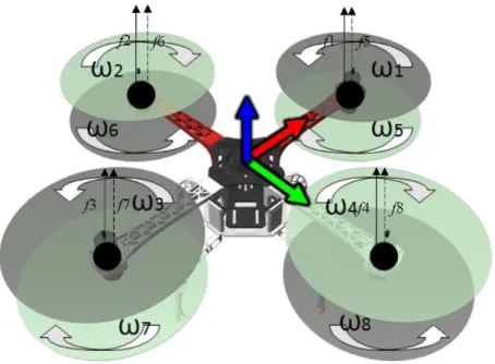
Figure 3.1: Representation of the quadrotor steady hovering. XYZ axes are repre-sented by RGB arrows, respectively. Retrieved from (Brito 2016).

On the Figure 3.1 illustrated above, are identified the angular speed 𝜔_𝑛and the respective force 𝑓_𝑛 produced by each rotor 𝑛. Particularly, this image illus-trates a hovering flight, since all forces have equal magnitude. In addition, con-trolling each rotor independently enables the control of each of the three funda-mental rotations: roll, pitch and yaw. The altitude and angular position control actuations are, therefore, mathematically represented by eq. (3.1.1).

[ 𝑈1 𝑈2 𝑈3 𝑈4 ] = [

∑8𝑛=1𝑓𝑛

𝑓4+ 𝑓8− 𝑓2− 𝑓6

𝑓3+ 𝑓7− 𝑓1− 𝑓5

𝑓1+ 𝑓3+ 𝑓6+ 𝑓8− 𝑓2− 𝑓4− 𝑓5− 𝑓7]

(3.1.1)

(46)

named attitude. The attitude and the translational position matrices are repre-sented by eq. (3.1.2) and (3.1.3), correspondingly.

𝚯𝑬 = [𝜙 𝜃 𝜓]𝑇 (3.1.2)

𝐏 = [𝑥 𝑦 𝑧]𝑇 _(3.1.3)

The first matrix refers to Euler angles and the second to the position seen from an inertial observer.

On Brito’s work, some of the aircraft parameters are explicitly referred, but others must be assumed to develop the control system. For detailed documenta-tion on the quadrotor inertial and geometric parameters see Attachment A.

3.1.2 Open-Loop system

Finally, it is presented the kinematics model represented by eq. (3.1.4), whose mathematical deduction and the model itself are found on Brito’s thesis (Brito 2016).

{

𝑥̈ = (sin(𝜙) sin(𝜓) + cos(𝜙) cos(𝜓) sin(𝜃))𝑈𝑀1

𝑦̈ = (cos(𝜓) sin(𝜙) − cos(𝜙) sin(𝜓) sin(𝜃))𝑈1

𝑀

𝑧̈ = −𝑔 + cos(𝜙) cos(𝜃)𝑈1

𝑀

𝜙̈ = ((𝐼𝑦𝑦− 𝐼𝑧𝑧)𝜃̇𝜓̇ − 𝐽𝑟𝜃̇Ω𝑟+ 𝐿𝑈2)_𝐼1_𝑥𝑥

𝜃̈ = ((𝐼𝑧𝑧− 𝐼𝑥𝑥)𝜙̇𝜓̇ − 𝐽𝑟𝜙̇Ω𝑟+ 𝐿𝑈3)_𝐼_𝑦𝑦1

𝜓̈ = ((𝐼𝑥𝑥− 𝐼𝑦𝑦)𝜙̇𝜃̇ + 𝐿𝑈4)_𝐼1

𝑧𝑧

(3.1.4)

In the previous system of equations, 𝑔 represents the gravity action, 𝐽_𝑟

[𝐾𝑔. 𝑚2_]_{each rotor inertia}_–_{eq. (3.1.5)}_–_and_Ω

𝑟 [𝑟𝑎𝑑. 𝑠−1] the sum of angular

(47)

𝐽

𝑟

=

𝑀 . 𝑟𝑟𝑜𝑡𝑜𝑟

2

2 (3.1.5)

Ω𝑟 = 𝜔1− 𝜔2+ 𝜔3− 𝜔4− 𝜔5+ 𝜔6− 𝜔7+ 𝜔8 (3.1.6)

The established relation between body axes rate and Euler angles rate im-plies two important limitations. First, it is only precise for one rotation at a time. If a second rotation is desired, the aircraft attitude must be carried to the origin state, assuming this state as (0,0,0). Second, and although an inequality is formed between the two reference frames, the model can be considered valid for narrow changes in attitude.

3.2 Extended Model

The issue with the simplified version is that the hovering fluctuations must not be neglectable, as they are relevant when the aircraft needs to perform rota-tions, e.g., on take-off and landing approach or in the presence of crosswinds. Another consideration is the presence of drag, associated to air resistance. There-fore, a distinction must be made between the body axes rate and the Euler angles rate. The deduction for the extended model version is presented throughout the following subsections.

3.2.1 Rotation Matrix

The root step of a rotating body modelling is to formulate, through mathe-matics, its own rotational dynamics. To accomplish this mathematical relation, the right-hand rule is applied to each axis of the Euclidean space system.

(48)

𝐑𝜙 = [

1 0 0

0 cos(𝜙) sin(𝜙)

0 − sin(𝜙) cos(𝜙)] (3.2.1)

𝐑𝜃 = [

cos(𝜃) 0 − sin(𝜃)

0 1 0

sin(𝜃) 0 cos(𝜃) ] (3.2.2)

𝐑𝜓 = [

cos(𝜓) sin(𝜓) 0

− sin(𝜓) cos(𝜓) 0

0 0 1

] (3.2.3)

𝑹𝜙 identifies roll rotation, 𝑹𝜃 pitch rotation and 𝑹𝜓 yaw rotation. With these

three vectors and applying the three elemental rotations in a given order, it is obtained a specific rotation matrix. For this work, it is chosen a XYZ intrinsic rotation convention. Multiplying the three elemental rotations, as 𝐑_𝛩 = 𝐑_𝜙𝐑_𝜃𝐑_𝜓, results in the rotation matrix described by eq. (3.2.4).

𝐑𝛩 = (3.2.4)

[sin(𝜙) sin(𝜃) cos(𝜓) − cos(𝜙) sin(𝜓) sin(𝜙) sin(𝜃) sin(𝜓) + cos(𝜙) cos(𝜓) sin(𝜙) cos(𝜃)cos(𝜃) cos(𝜓) cos(𝜃) sin(𝜓) − sin(𝜃) cos(𝜙) sin(𝜃) cos(𝜓) + sin(𝜙) sin(𝜓) cos(𝜙) sin(𝜃) sin(𝜓) − sin(𝜙) cos(𝜓) cos(𝜙) cos(𝜃)]

Important is to notice that 𝐑_𝛩 is an orthogonal matrix, meaning that 𝐑_𝛩−1 =

𝐑𝛩𝑇. This relation is relevant for applications seen ahead.

3.2.2 Newton-Euler equations of motion

(49)

{𝐅 = 𝑀𝐚 + 𝛀 × (𝑀𝐕)_{𝛕 = 𝐈𝛂}

𝒓+ 𝛀 × (𝐈𝛀) (3.2.5)

{𝐅 = 𝐓 − 𝐅_{𝛕 = 𝐓} 𝑔− 𝐅𝐷 + 𝛀 × (𝑀𝐕)

𝝉+ 𝛕𝐺𝑦𝑟𝑜+ 𝛀 × (𝐈𝛀) (3.2.6)

The eq. (3.2.6) is an extended expression of eq. (3.2.5). In these equations,

𝐅 = [𝐹𝑥 𝐹𝑦 𝐹𝑧]𝑇 represents the force, 𝛕 = [𝜏𝑥 𝜏𝑦 𝜏𝑧]𝑇 the momentum, a

[𝑚. 𝑠−2_]_{the acceleration,}_𝜶

𝒓 [𝑟𝑎𝑑. 𝑠−2] the angular acceleration, v the velocity, 𝛀

[𝑟𝑎𝑑. 𝑠−1_]_{the angular velocity, T is the thrust, Fg the gravitational force, FD the}

drag force caused by air resistance and τGyro the momentum generated due to the gyroscopic effect. The external products that appears in the equations are relative to the centrifugal and centripetal forces, respectively. Because this type of aircraft is assumed to be symmetric, the inertial moment matrix 𝐈 is defined as shown in eq. (3.2.7).

𝐈 = [𝐼𝑥𝑥0 𝐼𝑦𝑦0 00

0 0 𝐼𝑧𝑧

] (3.2.7)

3.2.3 Open-Loop System

First, we take in consideration only the aircraft reference frame. By this light, both linear and angular velocity vectors are given by eq. (3.2.8) and (3.2.9), respectively.

𝐕 = [𝑢 𝑣 𝑤]𝑇 _(3.2.8)

𝛀 = [𝑝 𝑞 𝑟]𝑇 _(3.2.9)

(50)

[𝐹𝐹𝑥𝑦

𝐹𝑧

] = [00 𝑈1

] − 𝐑𝛩[

0 0 𝐹𝑔

] − 𝐾𝑣[

𝑢 − 𝑊𝑥

𝑣 − 𝑊𝑦

𝑤 − 𝑊𝑧

] − 𝑀 [−𝑝𝑤 + 𝑢𝑟𝑞𝑤 − 𝑣𝑟 𝑝𝑣 − 𝑢𝑞 ]

[ 𝜏𝜙

𝜏𝜃

𝜏𝜓] = [

𝐿𝑈2

𝐿𝑈3

𝐿𝐶𝑑

𝐶𝑙𝑈4

] + 𝛕𝑔𝑦𝑟𝑜− [

(𝐼𝑧𝑧− 𝐼𝑦𝑦)𝑞𝑟

(𝐼𝑥𝑥− 𝐼𝑧𝑧)𝑝𝑟

(𝐼𝑦𝑦− 𝐼𝑥𝑥)𝑝𝑞

]

(3.2.10)

On eq. (3.2.10), 𝐶_𝑙is the lift coefficient, 𝐾_𝑣 [𝑘𝑔. 𝑠−1] is any appropriate di-mensioned variable associated with velocity and 𝑊_𝑥, 𝑊_𝑦 and 𝑊_𝑧 concerns the air flow on the three axes.

Now it is possible to characterize the model attending the body inertial frame, so the gyroscopic effect momentum 𝛕_{𝑔𝑦𝑟𝑜} is given by eq. (3.2.11).

𝛕𝑔𝑦𝑟𝑜 = 𝐽𝑟Ω𝑟(𝛀 × [

0 0

1]) = 𝐽𝑟Ω𝑟[ 𝑝 −𝑞

0 ] (3.2.11)

Although eq. (3.2.10) works, it has a setback. This system has six outputs to control. However, of all the six degrees of freedom possible for this system, the horizontal motion along the X and Y axes are not directly controlled by any of the four command inputs, leading to an underactuated system with only four degrees of freedom. Thus, raising issues on stability level. The solution to this problem is to combine the inertial, in this case the earth, reference frame with the aircraft body axes. Therefore, and knowing that 𝑹_𝛩 is an orthogonal matrix, the translational motion regarding earth is shown by eq. (3.2.12).

[𝐹𝐹𝑥𝑦

𝐹𝑧

] = 𝑹𝛩𝑇[

0 0 𝑈1

] + [00 𝐹𝑔

] − 𝐾𝑣[

𝑥̇ − 𝑊𝑥

𝑦̇ − 𝑊𝑦

𝑧̇ − 𝑊𝑧

] (3.2.12)

(51)

[𝑀𝑥̈𝑀𝑦̈

𝑀𝑧̈] = 𝐑𝛩

𝑇_[0₀

𝑈1

] + [ 00

−𝑀𝑔] − 𝐾𝑣[

𝑥̇ − 𝑊𝑥

𝑦̇ − 𝑊𝑦

𝑧̇ − 𝑊𝑧

]

[𝐈𝑝̇𝐈𝑞̇ 𝐈𝑟̇] = [

𝐿𝑈2

𝐿𝑈3

𝐿𝐶𝑑

𝐶𝑙 𝑈4

] + 𝐽𝑟Ω𝑟[

𝑝 −𝑞

0 ] − [

(𝐼𝑧𝑧− 𝐼𝑦𝑦)𝑞𝑟

(𝐼𝑥𝑥− 𝐼𝑧𝑧)𝑝𝑟

(𝐼𝑦𝑦− 𝐼𝑥𝑥)𝑝𝑞

]

(3.2.13)

Solving the system of equations concerning linear and angular accelerations and as functions of input commands, results in the open-loop system fully actu-ated expressed by eq. (3.2.14).

{

𝑥̈ = (cos(𝜙) sin(𝜃) cos(𝜓) + sin(𝜙) sin(𝜓))𝑈𝑀1− 𝐾𝑣(𝑥̇ − 𝑊𝑥)

𝑦̈ = (cos(𝜙) sin(𝜃) sin(𝜓) − sin(𝜙) cos(𝜓))𝑈1

𝑀 − 𝐾𝑣(𝑦̇ − 𝑊𝑦)

𝑧̈ = cos(𝜙) cos(𝜃)𝑈1

𝑀 − 𝑔 − 𝐾𝑣(𝑧̇ − 𝑊𝑧)

𝑝̇ = ((𝐼𝑦𝑦− 𝐼𝑧𝑧)𝑞𝑟 − 𝐽𝑟𝑞𝜔 + 𝐿𝑈2)_𝐼1

𝑥𝑥 𝑞̇ = ((𝐼𝑧𝑧− 𝐼𝑥𝑥)𝑝𝑟 − 𝐽𝑟𝑝𝜔 + 𝐿𝑈3)_𝐼1

𝑦𝑦 𝑟̇ = ((𝐼𝑥𝑥− 𝐼𝑦𝑦)𝑝𝑞 + 𝐿𝑈4)_𝐼1

𝑧𝑧

(3.2.14)

According to the previous equation, the body angular acceleration is subject to control. This control is performed directly over its attitude. Therefore, the body attitude matrix is, in this work, represented by eq. (3.2.15).

𝚯𝐴 = [𝛼 𝛽 𝛾]𝑇 (3.2.15)

The subscript 𝐴 denotes the aircraft frame.

3.2.4 Euler angle and body axis rates

(52)

[𝑝𝑞

𝑟] = 𝐈3𝑥3[ 𝜙̇

0

0] + 𝐑𝜙 [0𝜃̇

0] + 𝐑𝜙𝐑𝜃[ 0 0

𝜓̇] (3.2.16)

[𝑝𝑞 𝑟] = [

1 0 sin(𝜃)

0 cos(𝜙) sin(𝜙) cos(𝜃) 0 − sin(𝜙) cos(𝜙) cos(𝜃)] [

𝜙̇ 𝜃̇ 𝜓̇]

(3.2.17)

Eq. (3.2.16) establishes a mapping from the inertial to the body reference frames through the Euler angles and body axes rates. This is the convention adopted in this work and commonly adopted on aeronautics, where the yaw ro-tation is performed first, then pitch and finally roll, after which the Euler angles rate is converted to the body axes rate (Stengel 2016). 𝐈_3𝑥3 denotes a 3𝑥3 identity matrix.

This conversion matrix is non-orthogonal, meaning that if 𝐐 ∈ ℳ_𝑛𝑛, ∀ 𝑛 ∈

ℕ∗_{, then}_𝐐−1_{≠ 𝐐}𝑇_{. If the inverse transformation is applied, we are now obtaining}

the Euler angles rate from the body axes rate.

[ 𝜙̇ 𝜃̇ 𝜓̇] = [

1 tan(𝜃) sin(𝜙) tan(𝜃) cos(𝜙)

0 cos(𝜙) − sin(𝜙)

0 sin(𝜙)_cos(𝜃) cos(𝜙)_cos(𝜃) _]_[ 𝑝

𝑞

𝑟]

(3.2.18)

(53)

3.3 Motor dynamics and configuration

Two specific experiment were conducted in (Brito 2016). One to obtain a mathematical representation of the E305 2312E BLDC motor behaviour. The other, to understand the improvement of a two-rotor configuration on each arm over a one-rotor configuration.

3.3.1 Motor dynamics

With the first experiment, the mathematical representation led to an output as a function of only one input. Any constant coefficients are already considered. Eq. (3.3.1) shows the TF, with unitary static gain, representative of the motors dynamics. Both input and output are expressed in units of force, where the first regards the desirable force and the second the one that is actually exerted by the motors.

𝐹𝑛(𝑠) = _𝑠₂_{+25.9384𝑠+47.6205}47.6205 (3.3.1)

3.3.2 One-motor vs two-motor configuration

(54)

Figure 3.2: One-rotor configuration.

Figure 3.3: Two-rotor configuration.

𝑓1𝑅(𝑡) = −37.288994𝑇𝑃𝑊𝑀3+ 172.286169𝑇𝑃𝑊𝑀2− (3.3.2)

−249.117605𝑇𝑃𝑊𝑀+ 115.291879

𝑓2𝑅(𝑡) = − 70.427872𝑇𝑃𝑊𝑀3+ 319.248999𝑇𝑃𝑊𝑀2− (3.3.3)

−461.320062𝑇𝑃𝑊𝑀+ 215.423951

On the two previous equations, 𝑓_1𝑅 and 𝑓_2𝑅 represent the force produced on each quadrotor arm in one-rotor configuration and two-rotor configuration, re-spectively, and 𝑇_𝑃𝑊𝑀 represents the PWM period.

(55)

From Fig. 3.3, we can see that the improvement in thrust about Fig 3.2 is minimal. The way to surpass this physical threshold relies in different technical characteristics of each motor components, such as, e.g., the propellers length or pitch. By implementing a two-rotor configuration, the torque produced by each arm end may be generated with a lower power supply when compared to the one-rotor configuration. One reason is the influence of the top motor, which in-creases the efficiency of the bottom one.

3.4 The landing Approach

Once the model of the quadrotor is completed and equipped with the re-spective physical properties, the next step is to approach the aircraft landing with a mathematical description of the physics involved and with certain assump-tions. In this section, only the physics are considerate.

3.4.1 Ground Effect

Firstly, let’s assume the aircraft is hovering near the target and is able to acquire its relative position. If it is sufficiently closer to the target, an aerody-namic effect called Ground Effect happens to occur. This effect is previously de-scribed and the original deduction is based on an aircraft of a single propeller, specifically a helicopter, whose mathematical representation is expressed by eq. (2.2.3) and eq. (2.2.4). In this work, these equations are assumed as a valid esti-mate to the quadrotor case and so are tested considering the quadrotor geometry.

3.4.2 Touchdown

(56)

the leg suffers deformation on impact moment. This deformation can be quanti-fied by relying on Hooke’s Law.

𝐹𝑠 = −𝐾𝑠𝑧 (3.4.1)

Of the mass-spring system expressed by eq. (3.4.1), 𝐹_𝑠 represents the force exerted on the spring, 𝐾_𝑠 [𝐾𝑔. 𝑠−2] the stiffness constant and z [m] the defor-mation, or stretch, quantity of the spring. The negative sign intends to indicate the opposite direction between the spring deformation and force exerted by the spring. This is a second order system and it is marginally stable. This means that, if this system suffers a disturbance, the spring will never cease its oscillating mo-tion. The solution is to add a damping element, hence turning into a mass-spring-damper system, as in the suspension system of an automobile.

𝑚𝑧̈ = −𝐾𝑠𝑧 − 𝐾𝑑𝑧̇ (3.4.2)

Eq. (3.4.2) is a more complete version of the previous one, where a damping factor, 𝐾_𝑑 [𝐾𝑔. 𝑠−1], is added. It represents the friction against the spring stretch direction, causing the spring to eventually return to its resting position.

This last equation is the one to apply to the existing model. Its quality in the representation of the quadrotor legs dynamics is put to the test on the Simulation and Results Chapter. Here, the behaviour of the quadrotor is studied assuming

𝐾𝑠 = 10000 𝐾𝑔. 𝑠−2 and 𝐾𝑑 = 100 𝐾𝑔. 𝑠−1. With the first assumption, the

quad-rotor legs are expected to deform about two millimeters, given the overall body mass.

In this thesis, only a flat surface is considered, on which is performed a pure vertical landing by the quadrotor. For this, the four legs are mathematically char-acterized by Hooke’s Law, previously mentioned.

3.4.3 Disturbances

(57)

in altitude, the more critical becomes the information about its position and atti-tude in relation to the target. The force applied by the air resistance to aircraft motion is given by eq. (2.2.2), but approximated to 𝐅_𝐷, as observed on eq. (3.2.6).

3.5 Flight control

In this section, are presented the control methodologies as well as the con-trol architectures for each of the six degrees of freedom. It is important to refer that some assumptions are made, which are described below.

All the physics quantities regarding the aircraft motion are read from ideals sensors. Clearly, this kind of sensors do not exist, but for simplification purposes they are considered. Because the rotor inertia is very small, is therefore consid-ered zero for simulation purposes.

The motors dynamics obtained via experimentation conducted on Brito’s work are considered. In his work, the control unit is an Arduino, which provides PWM signals to control each motor. Thus, this time signal is converted to a force quantity that is described by eq. (3.3.2) or eq. (3.3.3), depending on the topology applied. In the simulation environment, the output of the control system in meas-ured in Newtons, so a conversion from force to time is necessary to preserve the characteristics of the real system. Fig. 3.4 illustrates this conversion under the form of a blocks diagram.

(58)

In the following control schemes, the motors’ dynamics and time / force re-lations are integrated.

3.5.1 PID controller

In the following subsections, the control schemes are composed by PID con-trollers due to their simplicity of implementation. To find the parameters, the Ziegler-Nichols tuning methods and the PSO algorithm are applied. These archi-tectures are structured in two stages: the inner loop, where the angular / linear speed is controlled; and the outer loop, where the position / attitude is locked at a desired setpoint. In this cascading control loop, the inner loop must be obvi-ously faster than the outer loop. The setpoint is applied to the outer loop, which is not able to eliminate inner loop disturbances, like drag. Also, an obvious reason lies with the fact that position is an integration of velocity, thus slowing down the system response to a positional setpoint.

PSO algorithm can have better performance than Ziegler-Nichols method on tuning the PID controllers as observed on (Yadav and BhuriaVijay 2015; Edaris and Abdul-Rahman 2016) works. Nonetheless, it may be difficult to find a local optimum that drives the system to a stable closed-loop or even to find a local minimum in the first place (Clerc and Kennedy 2002). Each particle may be driven away from a satisfactory solution depending on its location when initial-ized or the location of the global best particle.

Infra are the procedures to take in order to acquire the controllers’ parame-ters, along with tables showing the values obtained for the same parameters.

3.5.1.1 PSO method

(59)

𝑈(𝑠) = 𝐾𝐸(𝑠) ∙ (1 +_𝑠𝑇1

𝑖+ 𝑠𝑇𝑑) (3.5.1)

For any continuous-to-discrete transformation, a sampling of 10 𝑚𝑠 and the bilinear – Tustin – transformation, eq. (3.5.2), are applied (K. J. Astrom and Wittenmark 1996) in order to preserve the dynamics of the continuous model. The resulting PID discrete controller is described by eq. (3.5.3).

𝑠 =

_𝑇2

𝑠

℥−1

℥+1 (3.5.2)

𝑈(℥) = 𝐾𝐸(℥) ∙ (1 + (𝑇𝑠

2 ℥+1

℥−1)

1

𝑇𝑖+ (

2

𝑇𝑠

℥−1

℥+1) 𝑇𝑑) (3.5.3)

Where ℥ represents the discrete domain, 𝑠 the Laplace domain and 𝑇_𝑠 is the sampling period. The continuous system model is also discretized, but for sim-plicity are assumed null disturbances and the physical properties are preserved as constants.

The PSO algorithm is configured with a sampling period of 10 𝑚𝑠, swarm population of 20 particles where each particle is initialized with a random value comprised between 0 and an arbitrary positive value, 1.49 for both adjustmemt coefficients and a maximum of 1000 cycles if the stop condition has not yet been met. The reference signal is a unit step function, changing from zero to one in ten milliseconds at second two. The time horizon is set in the range [0; 10]𝑠 and sam-pling frequency of 100 samples per second. Throughout the next experiments, no restrictions were superimposed on the acquisition of the solutions.

The cost function chosen is a ponderation between the mean-squared error and a mean square variation of the control action and is represented by eq. (3.5.4).

𝐽(. ) = (𝛼 ∑ (𝑟𝑒𝑓(𝑘) − 𝑦(𝑘))𝑁 2

𝑘 + (3.5.4)

+𝛽 ∑ (𝑢(𝑘) − 𝑢(𝑘 − 1))𝑁 2

𝑘 )_𝑁1

(60)

solutions converges, the process ends and the solution is a local minimum or is very close to one.

Table 3.1 represents the PD and PID parameters obtained through PSO al-gorithm to control the roll / pitch angular speed. This continuous model must be also discretized.

Table 3.1: Roll / pitch controllers’ gains obtained via PSO method.

Roll / Pitch Kp Ki Kd

PD 1.7908 - 0.4907

PID 2.1672 5 0.4418

Where 𝐾_𝑝 = 𝐾, 𝐾_𝑖 =_𝑇𝐾

𝑖 and 𝐾𝑑 = 𝐾𝑇𝑑. With these parameters, a step signal is applied to the closed-loop system. The result is illustrated on Fig. 3.5.

Figure 3.5: Step response to pitch / roll speed closed-loop system. Controller’s gains based on PSO method.

It is possible to see that PD controller provides a reduced rising and settling time compared to PID controller.

(61)

Also, the sampling period used to discretize the continuous model affects the analytical discrete model precision. Higher the sampling rate, more similar are the continuous and discrete systems’ response to an input. However, as the coef-ficients become smaller, the more precision may be required. In the case of hori-zontal motion, where the respective control is placed on top of the attitude con-trol block, this situation is more evidenced. Consequently, the concon-trollers’ pa-rameters for the horizontal motion and altitude are ruled by Ziegler-Nichols Ul-timate Sensitivity method.

3.5.1.2 Ultimate Sensitivity method

The main idea behind this heuristic method lies in increasing progressively a sensitivity gain until the system reaches the threshold of stability. At this point, the sensitivity gain is given by 𝐾_𝑢 and the oscillatory reaction of the system pos-sesses a period given by 𝑇_𝑢 (Ziegler and Nichols 1995). Table 3.2 represents each controller’s gains obtained according predefined rules.

Table 3.2: Controllers’ gains obtained via Ultimate Sensitivity method.

Controller K Ti Td

P 0.5𝐾_𝑢 - -

PI 0.45𝐾_𝑢 𝑇_𝑢/1.2 -

PD 0.8𝐾_𝑢 - 𝑇_𝑢/8

PID 0.6𝐾_𝑢 𝑇_𝑢/2 𝑇_𝑢/8

(62)

The process to determine the controllers’ gains is here presented with the ascension speed control. The first step is to drive the closed-loop to the limit of stability and find 𝐾_𝑢 and 𝑇_𝑢. The marginally stable system is illustrated on Fig. 3.6.

Figure 3.6: Marginally stable ascension speed closed-loop system.

With this test, it is obtained 𝐾_𝑢 = 32.5 and 𝑇_𝑢 = 0.82𝑠. Applying the rules of Table 3.2, it is possible to design the controller. Fig. 3.7 illustrates the closed-loop system with PD and PID control over the ascension speed to understand which provides the fastest response.

Figure 3.7: Step response to ascension speed closed-loop system. Controller’s gains based on Ultimate Sensitivity method.

(63)

pro-3.5.2

Attitude control

The first control scheme presented regards the quadrotor attitude. The closed-loop system assumes a cascading control loop with one inner loop and an outer loop. The inner loop, as mentioned, must be faster than the outer loop, as it will set the stall speed response of the system. The control loop is illustrated on Fig. 3.8.

Figure 3.8: Attitude control scheme.

In order to maintain stability, a range of [−30; 30] degrees is set as admissi-ble for each angular position, thus restrained between these bounds. Under or above this range, the quadrotor stability and lift could be at risk.

The attitude controllers’ gains are obtained through PSO method. On the

(64)

Table 3.3: Attitude controllers’ gains obtained via PSO method.

Controller Kp Ki Kd

Roll speed 1.7908 - 0.4907

Pitch speed 1.7908 - 0.4907

Yaw speed 2.3375 - 0.6894

𝜶 1.5018 - -

𝜷 1.5018 - -

𝜸 0.988 - -

3.5.3 Position control

3.5.3.1 Altitude

The altitude is an important measure to control, as it is the core step to air-craft stabilization and motion. The closed-loop architecture adopted is illustrated by the following Fig. 3.9 and is similar to the one applied for attitude control.

Figure 3.9: Altitude control scheme.

For both speed and position control on Z axis, the controllers’ gains are

(65)

control. Table 3.4 shows the gains obtained by applying the Ultimate Sensitivity method to altitude control.

Table 3.4: Altitude controllers’ gains obtained via Ultimate Sensitivity method.

Speed 26 - 2.665

Position 2.065 - -

3.5.3.2 X / Y control

The way to control longitudinal and lateral positions is naturally different from the way to control the altitude. To move along X or Y axes, the quadrotor must suffer an inclination, be it pitch or roll, respectively. Therefore, in these cases, a control over attitude is needed. On Fig. 3.9 is represented the control ar-chitecture for X and Y positions.

Figure 3.10: Position control scheme.

(66)

angle setpoint to the inner loop. Finally, the outer loop is composed by the posi-tion control, where the posiposi-tion command, from a human controller or a high-level architecture, is applied.

On Table 3.5 are specified the controllers’ parameters for speed and position control, obtained through Ziegler-Nichols method.

Table 3.5: Position controllers’ gains obtained via Ultimate Sensitivity method.

X speed 0.7 0.392 0.098

Y speed 0.7 0.392 0.098

X 0.31 - -

Y 0.31 - -

3.5.4 Thrust control

One real limitation is the maximum amount of thrust that each motor can generate and provide to the body lifting. Obviously, the minimum thrust is zero, assuming air flow through the rotors is always forced down when they are pow-ered and the blades are rotating. From the simulation point of view, this is char-acterized by a saturation block. However, even if the output is limited, the system integrators keep accumulating the saturated value. This can lead to faulty actua-tions, influencing the overall system response. To diminish this effect, an anti-windup technique is applied.

(67)

(68)

(69)

4 Simulations and Results

In this chapter are presented all the tests conducted on the overall system. It is a way to validate all the work done on Chapter 3.

Througout the next sections and for testing purposes, a variable setpoint and a time horizon in the range of [0; 90]𝑠 are considered when only one rotation or translation is tested at a time. Also, each motors TF is contemplated and di-rectly influence the results.

For a more direct analysis and easy reading of the graphs, the angular units are expressed in degrees.

(70)

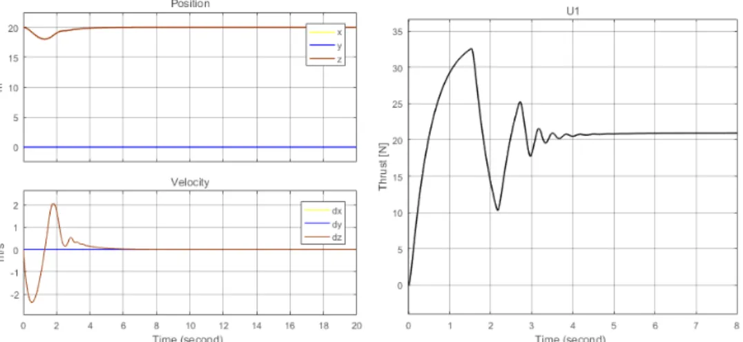
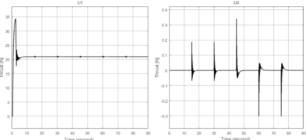
Figure 4.1: Hovering. From left to right, position and altitude control action.

Because at the start of the simulation the motors are at rest, the spikes on the right graph relate to the altitude control actuation over the motors, so the quadrotor remains at 20m setpoint, as seen on the left upper graph on the figure. The image from below refers to the speed at each time instant. In all figures where attitude or position are displayed, the respective velocities are illustrated below. The quadrotor must be hovering sufficiently away from the ground to ena-ble its rotation. Thus, the simulations are conducted on the aircraft while hover-ing at 20 m. The simulation starts with all motors off, hence the initial spikes cor-responding to the transient state.

4.1 Zero drag effect

The set of graphs analysed during this sub-chapter, do not contemplate any influence of any kind of disturbance. On the next one, some tests are then exe-cuted considering the effect of air resistance to linear motion.

4.1.1 Attitude

(71)

separa-4.1.1.1

Pitch rotation

The first step consisted in testing only one rotation at a time. Because the controllers for both pitch and roll are the same, are here presented only the pitch curves, as well as the control action.

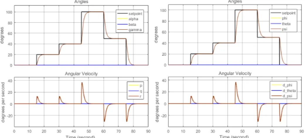
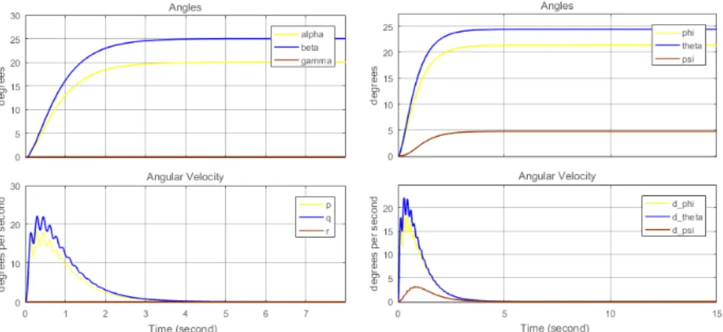
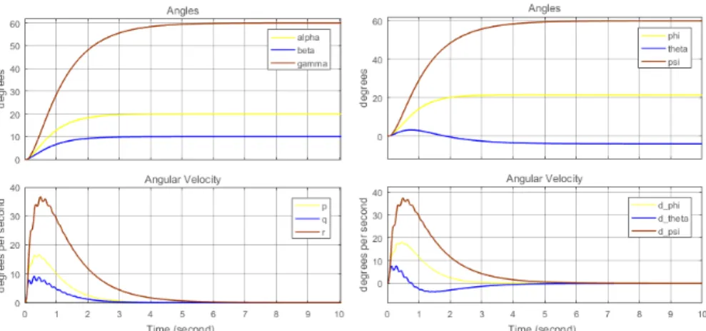
Fig. 4.2 illustrates the evolution of the angular displacement and rate of change over time. Because the specified limit to pitch and roll rotations are 30 degrees, the maximum setpoint applied is 25 degrees. The respective control ac-tion and the influence on altitude control actuaac-tion are presented on Fig. 4.3.

Figure 4.2: Rotation response to a variable pitch setpoint. From left to right, body and Eu-ler angles.

Quadrotor Simulator for Control De- velopment – Application to Autono- mous Landing

Ricardo dos Santos Moreira