Autonoumous Nervous System biosignal processing via EDA and HRV from a wearable device

Rodrigo Olival Lima

Bachelor Degree in Biomedical Engineering Sciences

Autonoumous Nervous System biosignal

processing via EDA and HRV from a wearable

device

Dissertation submitted in partial fulfillment of the requirements for the degree of

Master of Science in Biomedical Engineering

Adviser:

Doutor Hugo Filipe Silveira Gamboa, Professor Auxiliar,

Universidade Nova de Lisboa - Faculdade de Ciências e

Tecnologia

Examination Committee

Chairperson: Professor Paulo António Martins Ferreira Ribeiro Raporteur: Doutora Carla Maria Quintão Pereira

Rodrigo Olival Lima

Bachelor Degree in Biomedical Engineering Sciences

Autonomous Nervous System biosignal

processing via EDA and HRV from a wearable

device

Dissertation submitted in partial fulfillment of the requirements for the degree of

Master of Science in

Biomedical Engineering

Adviser: Prof. Dr. Hugo Gamboa, Auxiliar Professor,

NOVA University of Lisbon

Autonoumous Nervous System biosignal processing via EDA and HRV from a wear-able device

Copyright © Rodrigo Olival Lima, Faculty of Sciences and Technology, NOVA University of Lis-bon.

The Faculty of Sciences and Technology and the NOVA University of Lisbon have the right, perpetual and without geographical boundaries, to file and publish this dissertation through printed copies reproduced on paper or on digital form, or by any other means known or that may be invented, and to disseminate through scientific repositories and admit its copying and distribution for non-commercial, educational or research purposes, as long as credit is given to the author and editor.

This document was created using the (pdf)LA_{TEX processor, based in the “novathesis” template[1], developed at the Dep. Informática of FCT-NOVA [2].}

To my Mother and Family,

A

C K N O W L E D G E M E N T S

Com o desfecho do meu percurso a aproximar-se, é fundamental dirigir umas palavras de agradecimento a todos aqueles que me acompanharam durante estes 5 anos.

Começo por destacar o papel do Prof. Dr. Hugo Gamboa, que como meu orientador de dissertação, possibilitou-me a oportunidade de realizar a minha dissertação na empresa PLUX – Wireless Biosignals, e orientou-me em situações de dúvida, removendo obstáculos durante o processo científico.

Não menos importante, tenho de agradecer ao aluno de doutoramento e investigador do LIBPHYS-UNL, Daniel Osório, que ao longo de toda a minha dissertação acompanhou-me diari-amente e sempre se disponibilizou para retirar dúvidas que apareciam, guiou-me pelo caminho correto em situações difíceis, e transmitiu-me uma quantia inestimável de conhecimento cien-tífico.

A realização da dissertação na empresa PLUX – Wireless Biosignals teve grande importân-cia na minha evolução tanto a nível pessoal como profissional, pois permitiu-me conhecer o ambiente empresarial, bem como adaptar-me e ter acesso ao mercado de trabalho durante o meu percurso académico.

Um agradecimento a todo o pessoal da PLUX, pelo ambiente descontraído e divertido que encontrei desde o momento em que comecei a minha dissertação, e por me acolherem de uma forma magnífica na empresa.

Em especial, gostaria de agradecer ao CEO Manuel Pacheco, que durante a dissertação incutiu tarefas que desafiaram a dar o melhor de mim, e pela disponibilidade e amabilidade que sempre demonstrou.

Aos membros da equipa de desenvolvimento de software, Rui Freixo, Gonçalo Telo, Maria Magalhães, André Lemos e Miquel Alfaras, um obrigado por me acompanharem durante estes últimos meses.

A toda a equipa de produção de hardware, em especial ao Paulo Aires que possibilitou toda a aquisição de sinal fisiológico através do dispositivo wearable. Agradecimento também à equipa do projeto LISA (Learning Analytics for Sensor-Based Adaptive Learning) que contribuíram para o desenvolvimento do dispositivo wearable.

Um agradecimento também à Prof. Dr. Claúdia Quaresma que me disponibilizou o labo-ratório na Faculdade de Ciências e Tecnologia, para recolha de dados a voluntários.

Esta dissertação realizou-se apenas no 2º semestre do último ano de faculdade, no entanto, o resto do meu percurso académico foi realizado com o apoio de um grupo de amigos durante 5 anos. Só eles sabem o que me custou estar estes 5 anos longe da família, e sem eles não conseguiria encontrar a motivação e alegria para continuar focado no meu objetivo.

Um agradecimento do fundo do coração para a Beatriz Barata, o Bernardo Gonçalves, a Inês Marques, a Maria Afonso, a Mariana Carvalho, o Pedro Moura, o Rui Varandas e o Tomás Pinheiro, vocês são a minha segunda família.

A todos os meus amigos de infância, especialmente ao Gonçalo Nóbrega que me acompan-hou durante os 5 anos na mesma faculdade, um agradecimento especial.

This is how you do it: you sit down at the keyboard and you put

one word after another until its done. It’s that easy, and that hard.

A

B S T R A C T

The assessment of changes in the autonomous nervous system (ANS) with certain diseases and pathologies conditions, has been demonstrated to have important prognostic and diagnostic value, so delineating the role of autonomous activity is important to prevent health diseases.

There are many approaches to directly measure the sympathetic and parasympathetic ner-vous system, although, most of them are invasive and unable to provide continuous monitoring, leading to inaccurate assessment of the autonomous nervous system.

Heart rate variability (HRV) and Electrodermal activity (EDA) are presented has noninvasive methods to assess the ANS, by computing the spectral analysis of both HRV and EDA biosignals. The combination of these signals is necessary to correctly measure the activity of the sympa-thetic and parasympasympa-thetic system, due to the fact that frequency analysis of HRV only provides the level of unbalance between these two systems, while EDA reflects only activity from the sympathetic system. ANS biosignal processing via HRV and EDA from a wearable device was studied in this thesis, in order to provide continuous monitoring. A wearable device is the ideal solution, as HRV can be calculated with photoplethysmography signals from the wrist and EDA from the fingers, providing wireless and continuous monitoring of the subjects.

The extraction of the HRV and EDA features, that describe the activity of the sympathetic and parasympathetic system, were obtained by submitting the subjects to a mental arithmetic stress test, and then compared to the baseline values, in order to verify changes in the au-tonomous nervous system between the two situations.

The distinct response to stress for the subjects was then predicted using machine-learning classification mechanisms, with the ability to predict how the subject will respond when sub-mitted to a situation of stress, using only time-domain features, instead of frequency-domain features, which reduces the time needed to perform the classification.

Keywords: Heart Rate Variability; Electrodermal Activity; Photoplethysmography; Biosignals;

R

E S U M O

A avaliação das alterações do sistema nervoso autónomo (SNA), associadas a determinadas doenças e patologias, têm vindo a ganhar um importante papel no prognóstico de doenças, daí a importância de delinear o papel da atividade do SNA na prevenção de doenças.

Atualmente, existem diversas técnicas para medir diretamente os sistemas nervosos sim-pático e parassimsim-pático, no entanto, a maioria destas técnicas são invasivas e não permitem a monitorização de forma contínua, o que leva a uma incorreta conclusão acerca das alterações no SNA.

A Variabilidade Cardíaca (VC) e a Atividade Eletrodérmica (EDA) surgem como métodos não invasivos para avaliar o SNA, através da análise espectral destes mesmos bio-sinais. A com-binação destes sinais é necessária para determinar de forma correta a atividade dos sistemas simpático e parassimpático, pois a análise espectral da VC apenas fornece informação sobre o balanço entre estes dois sistemas, enquanto que a EDA apenas reflete a atividade do sistema simpático. De forma a colmatar o problema da monitorização contínua, um dispositivo wea-rable foi utilizado, medindo a VC através da fotopletismografia no punho, e a EDA nos dedos da mão. A computação dos parâmetros de VC e EDA que descrevem a atividade do sistema nervoso, foram obtidos, submetendo os participantes a um teste de stress aritmético mental, comparando os valores em situação de repouso com os valores obtidos em situação de stress, de forma a verificar alterações no SNA.

As distintas respostas dos participantes, quando submetidos a uma situação de stress, fo-ram previstas através de mecanismos de classificação, de forma a prever de que maneira os participantes respondem a uma situação de stress, utilizando apenas parâmetros calculados no domínio do tempo, o que reduz significativamente o tempo necessário para efetuar uma classificação do tipo de resposta de cada pessoa.

Palavras-chave: Variabilidade Cardíaca; Atividade Eletrodérmica; Fotopletismografia; Bio-sinais;

C

O N T E N T S

List of Figures xxi

List of Tables xxiii

Acronyms xxv

1 Introduction 1

1.1 Context . . . 1

1.2 Goals . . . 3

2 Theoretical Concepts 5 2.1 Autonomous Nervous System . . . 5

2.2 Photoplethysmography (PPG) . . . 7

2.3 Heart Rate Variability (HRV) . . . 8

2.3.1 HRV Concepts . . . 8

2.3.2 Time domain methods . . . 8

2.3.3 Frequency domain methods . . . 11

2.4 Electrodermal Activity (EDA) . . . 12

2.4.1 EDA Concepts . . . 12

2.4.2 EDA Measurement . . . 13

2.4.3 EDA Models . . . 14

2.4.4 EDA Processing . . . 16

2.5 HRV and EDA relationship: Review . . . 17

2.6 Paced Auditory Serial Addition Test (PASAT) . . . 17

2.7 Statistical Analysis . . . 19

2.7.1 Kruskal-Wallis test . . . 19

2.7.2 Chi-square test for Goodness of Fit . . . 20

2.8 Support Vector Machines (SVM) . . . 21

3 Materials and Procedure 25

3.1 Study Population . . . 25

3.2 Wearable Device . . . 25

3.3 Acquisition Protocol . . . 26

3.4 Software . . . 28

4 Data Processing 29 4.1 HRV . . . 29

4.1.1 Peak Detection Algorithm for PPG . . . 30

4.1.2 Heart Rate Computation . . . 31

4.1.3 RR-interval series filtering . . . 32

4.1.4 Statistical Variables . . . 33

4.1.5 Non-linear Variables . . . 33

4.1.6 Frequency Components . . . 34

4.2 EDA . . . 35

4.2.1 EDA Pre-Processing . . . 35

4.2.2 SCL . . . 35

4.2.3 SCR Features . . . 36

4.2.4 Frequency Analysis . . . 37

5 Results 39 5.1 EDA Features . . . 39

5.1.1 Time-domain Analysis . . . 39

5.1.2 Frequency-domain Analysis . . . 40

5.2 HRV Features . . . 45

5.2.1 Time-domain Analysis . . . 45

5.2.2 Frequency-domain Analysis . . . 48

5.3 HRV Non-linear Variables Boxplots . . . 51

5.4 Kruskal-Wallis test . . . 52

5.4.1 EDA Kruskal-Wallis test . . . 53

5.4.2 HRV Kruskal-Wallis test . . . 53

5.5 Group 1 Features . . . 54

5.5.1 HRV Features . . . 54

5.5.2 EDA Features . . . 54

5.6 Group 2 Features . . . 55

5.6.1 HRV Features . . . 55

5.6.2 EDA Features . . . 55

5.7 Groups Separation . . . 56

5.8 Classification . . . 58

5.8.1 HRV features Random Forest Classifier . . . 58

C O N T E N T S

6 Discussion 65

7 Future Expectations 67

Bibliography 69

A Appendix A - HRV Features 77

B Appendix B - EDA Features 81

C Appendix C - Group 1 HRV Features 87

D Appendix D - Group 2 HRV Features 91

E Appendix E - Group 1 EDA Features 95

F Appendix F - Group 2 EDA Features 101

G Appendix G - EDA Features Kruskal-Wallis test 107

H Appendix H - EDA Groups Kruskal-Wallis test 109

I Appendix I - HRV Random Forest Classifier 113

J Appendix J - HRV and EDA Random Forest Classifier 115

L

I S T O F

F

I G U R E S

2.1 Schematic of the autonomous nervous system . . . 6

2.2 Schematic of the synaptic transmitter substances . . . 6

2.3 Photoplethysmogram pulse waveform . . . 7

2.4 HRV triangular index . . . 10

2.5 Poincaré Plot . . . 11

2.6 Electrodermal activity . . . 12

2.7 Skin Conductance Response . . . 13

2.8 Skin Conductance Level . . . 13

2.9 Proposed SCR event model. . . 15

2.10 SCR component derivatives . . . 15

2.11 Synchronization in the increase of EDA and heart rate . . . 17

2.12 Flow of the Paced Auditory Serial Addition Test (PASAT) . . . 19

2.13 SVM Hyperplane . . . 23

2.14 Structure of a Decision Tree . . . 24

2.15 Structure of a Random Forest Classifier . . . 24

3.1 Wearable Device . . . 26

3.2 Visualization of the Recording Sites . . . 27

3.3 Digit Presentation in PVSAT . . . 27

3.4 Representation of the warning and start of the PVSAT . . . 28

4.1 HRV data segmentation . . . 29

4.2 Comparison between PPG raw signal and filtered . . . 31

4.3 Peaks Detected in PPG . . . 31

4.4 Normal Heart Cycle . . . 32

4.5 RR series linear interpolation . . . 33

4.6 HRV power spectrum . . . 35

4.7 EDA data segmentation . . . 36

L

I S T O F

T

A B L E S

A

C R O N Y M S

ANOVA Analysis of Variance.

ANS Autonomous Nervous System.

B1 Baseline 1 (0-min to 2-min). B2 Baseline 2 (2-min to 4-min). Bpm Beats-per-minute.

ECG Electrocardiogram. EDA Electrodermal Activity.

EDASympn Electrodermal Activity Sympathetic tone.

FFT Fast Fourier Transform.

GSR Galvanic skin response.

HF High Frequency. HRV Heart Rate Variability.

Hz Hertz.

IHR Instantaneous Heart Rate. ISI Inter-stimuli interval.

LED Light-Emitting Diode. LF Low Frequency.

n.u normalized units. NN Normal-to-Normal.

NN50 Number of interval differences of successive NN intervals greater than 50 ms.

PASAT Paced Auditory Serial Addition Test. PGR Psycho-galvanic reflex.

pNN50 Proportion of NN50.

PNS Parasympathetic Nervous System. PPG Photoplethysmography.

PSD Power spectral density.

PVSAT Paced Visual Serial Addition Test.

RMSSD Square root of the mean squared differences of successive NN intervals.

s seconds.

S1 Stress 1 (6-min to 8-min). S2 Stress 2 (8-min to 10-min). SCL Skin conductance level. SCR Skin conductance response.

SDANN Standard deviation of the average NN interval. SDNN Standard deviation of the NN interval.

SDRR Standard deviation of RR intervals.

SDSD Standard deviation of the successive differences. SE Standard Error.

SNS Sympathetic Nervous System. SSR Sympathetic skin response. SVM Support Vector Machine.

TBI Traumatic brain injury.

TINN Triangular interpolation of NN interval histogram. TVOC Total volatile organic compound.

ULF Ultra-Low Frequency.

C

1

I

N T R O D U C T I O N

1.1 Context

In the past years there has been a significant relationship between the autonomous nervous system (ANS) and cardiovascular research [1]. The assessment of the changes in the sympa-thetic and parasympasympa-thetic activity of the ANS with certain diseases and pathologies, such as myocardial infarction, cardiac transplantation, myocardial dysfunction, diabetic neuropathy and depression, has been demonstrated to have important prognostic and diagnostic value [1]. Given this relationship, delineating the role of autonomous cardiac reactivity is important to prevent these serious health conditions. The autonomous nervous system is regulated by the central autonomous network in the brain, comprised of multiple neuroanatomical structures which receives input regarding the internal and external environment. These brain related structures influence heart activity, responding and adapting to environmental challenges and self-regulate, each influencing the heart in a different manner, actuating mainly on the sinoa-trial node of the heart [2]. The autonomous control is transmitted to the organs of the body through two divisions of the ANS: the sympathetic nervous system (SNS) and the parasym-pathetic nervous system (PNS). The two systems of the ANS influence the heart in different ways. The parasympathetic system influences the heart through the vagus nerve, which mainly decreases the heart rate. Stress usually withdraws vagal activity, decreasing control of the heart via the vagus nerve. This facilitates the activation of the sympathetic system. The sympathetic system is associated with excitatory influences on the heart, resulting in an acceleration of heart rate [2].

represented by the R peak in the QRS complex of the ECG [8]. HRV can also be computed by acquiring photoplethysmography (PPG) signals, which are an optical measurement technique with widespread clinical application, such as ambulatoy patient monitoring, used to detect blood volume changes in the microvascular bed of tissue. PPG signals are a source of heart rate information, since there is a correlation between heart beats and a blood volume change. These signals are already being applied in many different clinical settings, including clinical physiological monitoring, vascular assessment, and autonomic function, such as HRV [9].

The heart rate is influenced by the autonomous nervous system, thus making HRV one of the most promising markers of autonomous activity, that allows to monitor the propensity for lethal arrhythmia and signs of either increased sympathetic or reduced vagal activity. Spectral analysis of HRV has been used to understand the modulatory effects of neural mechanisms. The parasympathetic activity is a major contributor to the high frequency (HF) component while the low frequency (LF) component is considered to be a marker of the sympathetic modulation when expressed in normalized units, but it is also influenced by the PNS [10]. The ratio between the LF and HF gives us information about the sympathetic and parasympathetic balance [11], but there is some conflicting ideas in academia about its power to be an accurate measure of the ANS since the LF component also contains information about the parasympathetic system [1].

An alternative method to directly assess the sympathetic nervous system is to measure and process electrodermal activity (EDA) [12]. This activity has been studied from two distinct theories: the vascular theory and the excretory theory. The vascular theory is based on the re-lationship between skin conductance changes and an increase in blood flow, implying a direct relationship between EDA and the circulatory system. This thesis will focus on the excretory theory, due to the relationship between EDA and the sympathetic branch of the ANS, stating that EDA is directly related to the sympathetic system [13]. The human skin is innervated by nu-merous efferent fibers, including sympathetic fibers for innervation of the eccrine sweat gland’s secretory segment. The eccrine glands in the skin produce sweat when the acetylcholine trans-mitter passes from sudomotor fibers to these glands, which means that sudomotor transmittion is cholinergic, increasing sweat concentration and thus changing the skin electrical characteris-tics [14]. Eccrine glands are mostly involved in emotional responses to external stimulus [15], and only reflect activity of the sympathetic nervous system, because there is no innervation of the PNS in these glands [16]. The magnitude of sweating depends on the density of sweat eccrine glands, which varies between individuals, thus the location where EDA is measured, is an important factor to take into account. Standard sites for EDA recording are palmar locations or finger phalanges [14], although several studies started to explore the measurement of EDA at other locations, such as feet, chest, neck, wrist and ankle [15].

1 . 2 . G O A L S

must be summed in a narrow time interval, triggering a state of anxiety and stress among the participants, changing sweat concentration and instantaneous heart rate, thus making it eas-ier to detect impairments in the parasympathetic and sympathetic nervous systems, due to neuropsychological syndromes.

The objective of this thesis is to analyze HRV and EDA features that describe the ANS. This work will make it possible to detect disorders in the ANS, identifying potential opportunities for clinical intervention such as prognostic or diagnosis of the diseases and pathologies named previously in this section. Finally, classification mechanisms will be applied to establish the level of unbalance between the parasympathetic and sympathetic system, in response to stress situations, mechanisms that should be validated in real use case environments.

This thesis is divided in 5 chapters. In chapter 2, theoretical concepts are presented in order to understand the basis of the ANS, PPG, HRV, EDA, PASAT, Support Vector Machines (SVM), Statistical analysis and the Random forest classifier. In chapter 3, the characterization of the study population, the description of the wearable device used, and the acquisition protocol are presented. In chapter 4, processing methods to analyze HRV and EDA features are presented, both in time-domain and frequency-domain methods. The results obtained in this thesis are presented in chapter 5, in which HRV and EDA features are calculated and their significance is analyzed with statistical tests. Also in this chapter, the separation of the subjects into two different groups according to the response to stress, is performed. Finally, a discussion of the results obtained are presented in chapter 6.

1.2 Goals

The goals of this thesis are: try to monitor the autonomous nervous system with a wearable device by processing HRV and EDA, induce stress to the participants and classify the level of stress of the participants.

The step-by-step goals to achieve the thesis objective are discriminated in the next items: 1. HRV and EDA familiarization and state-of-the-art;

2. Methods for extracting HRV and EDA; 3. Design a data acquisition protocol; 4. Data collecting using a wearable device; 5. Processing HRV and EDA data;

6. Analyze features from HRV and EDA in baseline and stress; 7. Classification of the data;

C

2

T

H E O R E T I C A L

C

O N C E P T S

2.1 Autonomous Nervous System

The autonomous nervous system is responsible for controlling arterial pressure, sweating, body temperature, heart rate, among others activities. One of the most striking characteristics of the ANS is the quickness and intensity with which it can increase heart rate to twice the normal (in 3 to 5 seconds) or induce sweating within seconds. The ANS is activated mainly by centers located in the spinal cord, brain stem and hypothalamus [17].

The autonomous signals are transmitted to the body through two branches of the ANS: the sympathetic nervous system (SNS) and the parasympathetic nervous system (PNS) (Fig.2.1). The sympathetic and parasympathetic nerve fibers secrete two synaptic transmitter substances: acetylcholine and epinephrine. The fibers that secrete acetylcholine are called cholinergic while those that secrete epinephrine are called adrenergic (a term derived from adrenalin). The terminal nerve endings of the parasympathetic system all secrete acetylcholine, thus its influence on heart rate is mediated via release of acetylcholine by the vagus nerve, while the terminal nerve endings of the sympathetic system secrete epinephrine (Figure 2.2), thus its influence on heart rate is mediated via release of this neurotransmitter [13, 17].

Figure 2.1: Schematic of the autonomous nervous system and its divisions into the parasym-pathetic and symparasym-pathetic systems. The release of the neurotransmitter acetylcholine by the parasympathetic system and epinephrine by the sympathetic system, affects the major organs shown in the schematic [18].

2 . 2 . P H O T O P L E T H Y S M O G R A P H Y ( P P G )

2.2 Photoplethysmography (PPG)

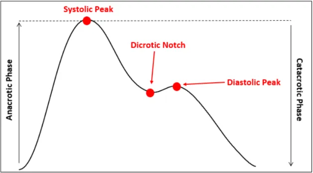
Photoplethysmography (PPG) is an optical measurement technique with widespread clinical application, used to detect blood volume changes in the microvascular bed of tissue. PPG re-quires the usage of only two opto-electronic components in order to acquire a signal: a light source (light-emitting diode) to illuminate the skin, and a photodetector to measure variations in light intensity associated with changes in perfusion. The amount of light received is influ-enced by key factors, such as blood volume, blood vessel wall movement and the orientation of red blood cells [9, 20]. The interaction of light with the skin is complex and involves processes such as, scattering, absorption, reflection, transmission and fluorescence. In this thesis, the configuration used to detect PPG is the reflection mode, where the LED and detector are placed side-by-side in the skin, and the signal received is the amount of light reflected, emphasizing that a good contact with the skin is necessary to acquire a clean signal, without excessive pres-sure, to avoid blanching. The PPG waveform pulse (Fig.2.3) is defined by the appearance of two phases: the anacrotic phase and the catacrotic phase. The anacrotic phase refers to the rising edge of the pulse, related to the systole, and the catacrotic phase refers to the diastole and wave reflections from the periphery. Also, a dicrotic notch is usually seen in the catacrotic phase in patients with healthy arteries [9]. Heart rate can be estimated by the difference between two consecutive systolic peaks.

2.3 Heart Rate Variability (HRV)

2.3.1 HRV Concepts

HRV is the study of the differences between consecutive heart beat, obtained from the time series of beat-to-beat intervals from an electrocardiogram (ECG) between consecutive heart beats, represented by the R peak in the QRS complex of the ECG [8]. An ECG is a time-series signal measured on skin surface which reflects the electrical activity of the heart [8]. It is ob-tained by recording the potential difference between two electrodes and a reference placed on the body surface, requiring a minimum of three electrodes connected with wires to the subject, to obtain an ECG recording.

The PPG signal reduces the number of contact surfaces to simply one wire, which is de-sirable for cardiac monitoring in ambulatory situations [20, 21]. Heart rate in a PPG signal is obtained by calculating the difference in time between two consecutive systolic peaks corre-sponding to the ventricular depolarization, and HRV can be infered from differences in heart rate [22–24]. There are several methods and features possible to extract from the information of HRV, as we will see in sections 2.3.2 and 2.3.3.

2.3.2 Time domain methods

Time domain methods are the simplest methods to perform. After removal of artifacts in RR intervals, these intervals are also called as normal-to-normal intervals (NN). From these two measurements, it is possible to calculate time variables, such as, the mean NN interval, the mean heart rate, the longest and the shortest NN interval, the standard deviaton of NN intervals and instantaneous heart rate (IHR), as well as statistical and geometrical features [10].

2.3.2.1 Statistical methods

From series of IHR or NN intervals, particularly those that are recorded over 5-min or 24h, more complex statistical time domain variables [8, 25–27] can be calculated such as:

• Standard deviation of the NN interval (SDNN)

• Standard deviation of the average NN interval (SDANN) • SDNN index

• RMSSD • NN50 • pNN50

2 . 3 . H E A R T R AT E VA R I A B I L I T Y ( H R V )

as the lowest frequency components in the 24h period recording, being influenced by both the SNS and PNS activity. The RMSSD is the square root of the mean squared differences of suces-sive NN intervals and is used to estimate the changes reflected in HRV by the PNS, the NN50 is the number of interval differences of successive NN intervals greater than 50 ms, and finally, the pNN50 is the proportion of dividing NN50 by the total number of NN intervals, and is closely correlated to the PNS [8, 10, 25, 28]. Another statistical variable is the standard deviation of the average NN interval (SDANN) calculated over periods of 5 min, which is an estimate of heart rate changes due to cycles longer than 5 min. The SDNN index is the mean of the 5 min SDNN calculated over 24h, measuring the variability due to cycles shorter than 5 min. These last two variables will no be included in this thesis, due to the length of the recordings chosen (5-min) [10].

2.3.2.2 Geometrical methods

The series of NN intervals can also be converted into a geometric pattern, such as the sample density distribution of NN intervals duration, the sample density distribution of differences between adjacent NN intervals and the Lorenz plot of NN intervals. There are three main approaches that are used in geometric methods:

1 - The geometric pattern is converted into the measure of HRV.

2 - The geometric pattern is interpolated by a mathematically defined shape.

3 - The geometric shape is classified into several pattern-based categories which represent different classes of HRV.

Figure 2.4: The HRV triangular index is calculated by dividing the number of all NN intervals by the maximum of the density distribution Y=D(X). The TINN is calculated by the difference between the values M and N (TINN=M-N)[10].

2.3.2.3 Nonlinear Geometrical Methods

2 . 3 . H E A R T R AT E VA R I A B I L I T Y ( H R V )

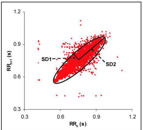
Figure 2.5: Poincaré Plot. SD1 - length of the transverse line. SD2 - length of the longitudinal line. The SD2/SD1 ratio reflects the nonlinear balance between the sympathetic and parasym-pathetic systems.

2.3.3 Frequency domain methods

In frequency-domain methods, power spectral density (PSD) analysis provides information on how the HRV is distributed in the frequency domain. These methods can be classified as non-parametric and non-parametric. The advantages of the non-non-parametric methods are: the simplicity of the algorithm employed (Fast Fourier Transform (FFT)) and the high processing speed.

2.4 Electrodermal Activity (EDA)

2.4.1 EDA Concepts

As mentioned in section 1.1, the human skin is innervated by numerous efferent fibers, in-cluding sympathetic fibers for innervation of the eccrine sweat gland’s secretory segment. The eccrine glands in the skin produce sweat when the acetylcholine transmitter passes from su-domotor fibers to these glands, increasing sweat concentration that changes the skin electrical characteristics [14], making it possible to measure EDA.

EDA (Fig.2.6) can be divided into the following components: skin conductance response (SCR),skin conductance level (SCL), sympathetic skin response (SSR), galvanic skin response (GSR) and the psycho-galvanic reflex (PGR). In this thesis, the signal will be divided in the SCL (tonic component) and the SCR (phasic component). The phasic component (Fig.2.7) is the result of the activation of the sympathetic system, after a stimulus presentation, being usually overlapped by the tonic component (Fig.2.8), which is not directly related to the presentation of the stimulus [31]. The skin conductance response (SCR) is composed by two zones: a rise zone and a decay zone. The rise zone starts at the initial instant (t0), and marks the moment

the sudomotor system reacts to the ANS. The rise time is defined as the time that it takes from the momentt0to reach the maximum of the rise zone,t2(Fig.2.10) [13].

2 . 4 . E L E C T R O D E R M A L A C T I V I T Y ( E D A )

Figure 2.7: Skin Conductance Response (SCR) component of the EDA signal.

Figure 2.8: Skin Conductance Level (SCL) component of the EDA signal.

2.4.2 EDA Measurement

EDA measurement is usually performed in the hand palm, particularly in the anterior part of the finger tips. In order not to disturb people while performing some task using the hands, it is common to place the electrodes on the non-dominant hand, given that EDA presents a symmetrical characteristic. Using the endosomatic approach (constant current) to measure the electrical mechanism, the sympathetic skin response is the result of a distinct processing path where the low frequencies (SCL) are typically obtained by band passing the signal in the 0.1−2

2.4.3 EDA Models

2.4.3.1 Modeling Difficulties

The two main difficulties encountered by EDA models in electrodermal events detection and quantification is the overlapping events and the occurrence of low amplitude events, leading to distorted values extracted for the events [32]. The problem of overlapping events in an SCR event occurs when an event ensues immediately after another SCR event, usually masking the real values of the event in the decay zone of the SCR peak. When an EDA event has low amplitude compared to the decreasing exponential of a previous SCR event, it will not be detected by either models based on visual detection or those that are based in the first derivative and zeros. In both these problems, the parameters of an SCR event will not be correctly extracted from the signal [13].

2.4.3.2 EDA Models

The modeling of the EDA has passed through several phases along its research history and tech-nological evolution. The first models to interpretate EDA signal were based on visual detection of skin conductance responses, where the observer manually annotated the time instants of the start of the events. This approach is considered to be a qualitative approach. With the improvement of computational resources, the next models applied to the EDA were based on the identification of the valleys and peaks of the signal. These models assumed the existence of two zones in a SCR event, that were computed by the signal derivatives and corresponding zero crossings. As with the latter, these models were unable to retrieve correct parameters in a case of an event overlap or in case of an event so smooth that does not have a peak or a valley. The sigmoid-exponential model proposed a set of models of increasing complexity, solving the problem of the overlapping SCR events, but the intrinsic problems of the optimization were still a problem, as the success a good fit to the model depended on the parameter initialization [13].

2.4.3.3 Model Applied

The proposed model [13] is based on a morphological study of the EDA signal. In order to detect the SCR component, this model applies signal filtering and computation of signal derivatives, eliminating the constant components, such as the SCL. The first step of the algorithm is to filter the signal with a lowpass butterworth 4th order filter (1 Hz). For simplicity of the model, it is assumed that the SCR event is isolated, with null SCL. After filtering, it is necessary to detect the second order derivative zeros, corresponding to the instantst1andt3as shown in Figure

2 . 4 . E L E C T R O D E R M A L A C T I V I T Y ( E D A )

being the unitary step function andk=4.

H(s)= α

(s+b)n (2.1)

Figure 2.9: Proposed SCR event model.

h(t)=L−1(_H(_s))=αtke−btu(t)=f(t)u(t) (2.2)

Next, for each pair of zeros (t1,t3), compute the parametersα,b,t0of the proposed model

given by equations 2.3,2.4,2.5, and finally compute the SCL component (Fig.2.8) by subtracting the detected events from the total EDA signal. This model is then, able to detect and quantify normal events, overlapping events and small events [13].

α=b3 f

′_(t

1)−f′(t3)

16e−2_+432e−6 (2.3)

b= 4

t3−t1 (2.4)

t0=3t1−t3

2 (2.5)

2.4.4 EDA Processing

2.4.4.1 Time Domain methods

EDA recording is based on relatively slow-changing and high latency physiological processes, so the analysis of EDA is mainly performed in time-domain methods, using the SCR and the SCL components. These latencies are normally between 1 and 2 seconds, but may be delayed up to 5 seconds in cases of skin cooling [14]. A measure of the amplitude of the EDA event is the most frequently metric, measuring an increase or decrease of the amplitude of the components of the EDA, due to a presentation of a stimulus after a certain latency [14]. Although these time domain methods are the most used procedures to analyse EDA, several studies have reported a high variability between subjects and low consistency when using time domain methods and therefore, frequency domain methods have been reported as a tool of sympathetic tone (EDASympn) assessment [4].

2.4.4.2 Frequency Domain methods

2 . 5 . H R V A N D E D A R E L AT I O N S H I P : R E V I E W

2.5 HRV and EDA relationship: Review

In a situation of induced stress, the balance of the PNS and SNS changes. The control mecha-nisms of the ANS to this stimuli, is a reduction of the parasympathetic activity and increase of sympathetic activity, leading to an increase in heart rate. EDA is known to be directly related to the dynamics of the cardiac and peripheral sympathetic nervous systems [33], so its association with HRV as been studied for the last years. The low frequency component of HRV provides in-formation about the sympathetic system, although it is also influenced by the parasympathetic system, so EDA gives us clear information about the sympathetic response to stress. Posada-Quintero et al.[1] showed that there was a considerable increase in the power spectra of the EDA in the same frequency range of the low frequency component of the HRV [1]. Kettunen et al. [34] showed that changes in EDA and heart rate, tend to exhibit interdependent changes in certain cognitive tests, as an acceleration in heart rate was synchronized with an increase in EDA level (although the increase in EDA was slightly later than the increase in heart rate, as shown in figure 2.11). This synchronization suggests that both EDA and heart rate are influ-enced by a common autonomic mechanism, such as the ANS [35]. Also, studies around specific pathologies, such as schizophrenia, showed that HRV and EDA are more interrelated than with control patients [36], so it is possible to monitor changes in the ANS through an EDA and HRV wearable device in patients with neural impairments.

Figure 2.11: Synchronization in the increase of EDA and heart rate [34].

2.6 Paced Auditory Serial Addition Test (PASAT)

2 . 7 . S TAT I S T I C A L A N A LY S I S

Figure 2.12: Flow of the PASAT [41].

2.7 Statistical Analysis

2.7.1 Kruskal-Wallis test

The Kruskal-Wallis 1-way analysis of variance by ranks is a non-parametric alternative test (H-test) to the 1-way ANOVA test. The 1-way ANOVA is used to determine whether there is any statistically significant difference between the means of two or more independent groups [42]. The null hypothesis of the ANOVA is that there is an absence of effect, such as no difference in the means between the baseline and the stress groups. The ANOVA produces an output, the F-value, which is a ratio between the "Between-group Variance"and the "Within-group Variance"(Eq.2.6), so a higherF-valueproduced means a large amount of variance between the

baseline and stress group, and a larger significant effect [43]. The ANOVA test has important assumptions that must be satisfied [44]:

• The samples are independent.

• The observations within each group are normally distributed. • The standard deviations of the groups are all equal (homoscedastic).

F−v al ue=Between-group Variance

Within-group Variance (2.6) The Kruskal-Wallis test is a non-parametric test, so it means that is does not assume the normal-ity of the data nor the homoscedaticnormal-ity. The H-test uses ranked values, so the values observed are converted to their ranks in the data set: the smallest value gets a rank 1, the next smallest gets rank 2, and so on. The Kruskal-Wallis null-hypothesis is that the mean ranks of the differ-ent groups are the same [45], so as in the ANOVA-test, ap-valuelower than the significance

level is better, concluding that the null hypothesis may not adequately explain the observation -there is in fact variation between the ranked means of each group. The level of significanceα

is chosen by the user, usually beingα=1%,5% or 10%. To quantify the statistical significance

better and that the null hypothesis may not adequately explain the observation. TheH-valueis computed with equation 2.7, if there are no ties (no two observations are equal)[46, 47].

H−v al ue= 12 N(N+1)

C

X

i=1 R2_i ni

−3(N+1) (2.7)

where:

C = the number of groups.

ni= the number of observation in theith group. N =P_n

ithe number of observations in all groups combined.

Ri = the sum of the ranks in theith group.

In case of ties, each observation is given the mean of the ranks for which it is tied, so the

H-valueneeds to be corrected (Eq.2.9), by dividing it by equation 2.8, where the summation is over all groups of ties [46, 47].

1−

P

T

N3−N, T=t

3_{−t with t = number of tied observations in the group (2.8)}

Ht i es=

H

1−_NP3_−NT

(2.9)

The degrees of freedom for the H-value are computed bydf1=C-1, where C is the number of groups (2: Baseline and Stress). The interpretation of the resultantH-valueis made by

com-paring it with the chi-square table. If there are more than five observations in each group, the

H-valueis distributed as a chi-square distribution with C-1 degrees of freedom -χ2(1) [47]. The

chi-square table shows that in order to obtain significant results (p-value<0.05) theH-value

must be higher than 3.84.

2.7.2 Chi-square test for Goodness of Fit

The chi-square test (χ2) is a test applied to determine whether a categorical variable from a

single population is consistent with a hypothesized distribution. It is applicable to many sit-uations in which experimental frequencies are compared to theoretical frequencies based on a hypothesis [48]. The null hypothesis for theχ2test is that the categorical data has the given

frequencies. This test has some assumptions that must be satisfied: the sampling method is simple random sampling, the variable is categorical and the expected value for the number of observations is at least 5. Theχ2statistic value is given by equation 2.10, where n is the number

2 . 8 . S U P P O R T V E C T O R M A C H I N E S ( S V M )

of freedom for theχ2value are computed byk−1−d d o f, wherekis the number of

observa-tions andd d o f is the adjustment to the degrees of freedom for thep-value, due to the linear regression performed, adding an extra constraint to the test (d d o f =1).

χ2=

n

X

i=1

·₍

Oi−Ei)2

Ei

¸

(2.10)

In the context of this thesis, theχ2test will be applied in section 5.7, to test the goodness of

the linear regression line performed [50], by comparing the values observed calculated using the regression line obtained, with the expected values. In this situation, by contrast with the Kruskal-Wallis test, it is better to obtain ap-valuehigher than the significance level, that is, we expect to accept the null hypothesis, so that the difference between the observed values and the expected values is minimized.

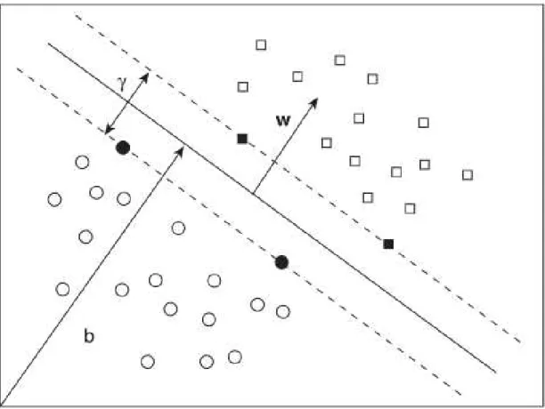
2.8 Support Vector Machines (SVM)

Support Vector Machines (SVM) were developed by Vapnik et al. from statistical learning theory and machine learning [51]. SVMs are a family of algorithms for learning two-class discriminat functions from a set of training examples, in order to find a suitable boundary (called a hyper-plane), in data space to separate the two classes. The basis of this boundary is the concept of margin, which is the minimal distance between the hyperplane separating the two classes and the closest points to it, defined as the support vectors. In linearly separable data, the kernel of SVM used is the maximal margin classifier or hard margin SVM. Considering a linearly separa-ble data sampleS={(x1,y1),...,(xi,yi)} whereiis the sample size, with a binary classification of the classes, such asY ={−1,1}, the support vectors are calculated based on equation 2.11 with a decision function given by equation 2.12 [52]. The pointsxare located in the hyperplane that

satisfies equation 2.11, where the support vectorswdefine a direction perpendicular to the hy-perplane, and the parameterbmoves the hyperplane parallel to itself, as shown in Figure 2.13 . For the two different classes, it is possible to define that the decision function has a positive and a negative value (±1), so considering two generic pointsx+andx−, that belong, respectively, to the positive and negative class, have a decision function given by equations 2.13 and 2.14. The marginγthat maximizes the distance between the hyperplane and the two classes, can

be achieved by minimizing the two-norm ofw[53]. The expression to calculate this margin is given by equation 2.15. All these parameters are represented in Figure 2.13.

〈w, x〉 +b=0, w, x∈Rn,b∈R (2.11)

f(x)=si g n(〈w, x〉 +b) (2.12)

〈w,x−〉 +b= −1 (2.14)

γ=

¿

w ∥w∥,(x

+

−x−)

À

= 2

2 . 9 . R A N D O M F O R E S T C L A S S I F I E R

Figure 2.13: Support Vector Machine - The hyperplane separates the data into two classes: circles represent class -1 and squares represent class +1. The bold circles and squares represent the support vectors. The marginγ, the parameter b and the vectors w, are also represented [53].

2.9 Random Forest Classifier

random forest classifier with 10 decision trees, if 6 out of 10 trees classify the data as belonging to group 1, the random forest will output that classification. The structure of a random forest classifier is shown in figure 2.15.

Figure 2.14: Structure of a Decision Tree [54].

C

3

M

A T E R I A L S A N D

P

R O C E D U R E

In this chapter, it’s described the wearable device used to acquire the EDA and PPG signals, as well as the software used to record and visualize the biosignals recorded. Also, a description of the acquisition protocol designed to implement the PVSAT is presented.

3.1 Study Population

Data was acquired from a group of healthy (reported) volunteer subjects. The total number of participants were fifteen (9 females and 6 males), ages from 21 to 55 years old (31 ± 11), height from 1.57 to 1.85 meters (1.73 ± 0.09) and weight from 52 to 94 kilograms (72 ± 13). This study was approved by FCT-UNL ethical committee and all subjects signed an informed consent. Table 3.1 gives the statistics for the study population.

Table 3.1: Study population characterization statistics for all subjects Mean STD Min Max

Age (years) 31 11 21 55 Height (m) 1,72 0,09 1,57 1,85 Weight (kg) 72 13 52 94

3.2 Wearable Device

is a green LED with a photodetector in reflection mode and the external EDA sensor uses Ag/Cl gel electrodes.

Figure 3.1: Wearable Device.

Table 3.2: Description of the wearable wrist device specifications.

Sensor Channel Resolution (bit) Sampling Rate

EDA wrist 1 10

10 Hz 100 Hz 1000 Hz

PPG 2 10

Spare 3 10

TVOC 4 10

CO2 5 6

TEMP 6 6

3.3 Acquisition Protocol

3 . 3 . A C Q U I S I T I O N P R O T O C O L

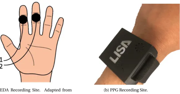
(a) EDA Recording Site. Adapted from [58].

(b) PPG Recording Site.

Figure 3.2: Visualization of the recording sites for both the PPG and EDA biosignals.

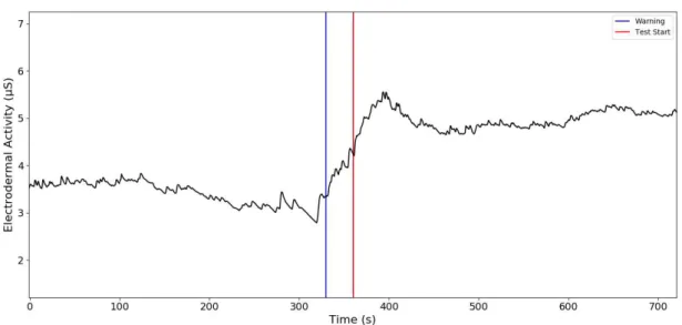
After placing the wearable device and the finger EDA sensor, the PVSAT test was explained to the subjects. Participants were presented with a series of single digits numbers and had to sum the two most recent digits, before the presentation of the next digit (see section 2.6). The PVSAT was performed to in the last 6-min, using a 12.2"tablet with white single numbers from 1 to 9, against a black screen (see Fig. 3.3). The digits were presented with a 3srate for the first 2min, decreasing half a second every two minutes (2.5sand 2s). The subjects had to respond

prior to the presentation of the next digit, and speak aloud each response. A 30s warning before the beginning of the PVSAT was given to all participants (Blue line in Fig. 3.4). During baseline measurements, the subjects were asked not to speak.

Figure 3.4: Representation of the warning and start of the PVSAT. EDA signal increases at the warning 30s before the PVSAT starts (Blue line). The start of the PVSAT is represented by the Red line.

3.4 Software

The software used to acquire the PPG and EDA data was PLUX’s OpenSignals software. This software is easy-to-use, versatile and allows real-time biosignals visualization, being capable of direct interaction with all PLUX’s devices via bluetooth. It is also capable to record simultaneous data for up to 24 channels, as well as loading pre-recorded signals.

C

4

D

A T A

P

R O C E S S I N G

4.1 HRV

The HRV data for all subjects was divided into two segments, one for each situation during the experiment: baseline and stress. As it is necessary to have 5-min recordings to compute frequency analysis of HRV, the baseline data goes from the start of the experiment to the 5th minute (Green band in Fig.4.1). The time between the 5th and the 7th minute (Red band in Fig. 4.1) was considered to be the transition band, where the heart rate changes significantly from baseline to stress, so this band was excluded. Finally, the stress data goes from the 7th minute, in which heart rate is already stable in the stress status, to the end of the experiment (Yellow band in Fig. 4.1). These bands are shown in Figure 4.1.

4.1.1 Peak Detection Algorithm for PPG

The algorithm implemented to detect a peak in a PPG wave is based on the algorithm used in [59]. The characteristic PPG wave is composed by two waves: the systolic wave corresponding to the systole and the dicrotic wave corresponding to the diastole. The valley between these two waves is called the dicrotic notch (Fig. 2.3). First, it is necessary to filter the signal in order to remove noise. The signal was filtered with a 2nd order lowpass Butterworth filter with the cutoff frequency set at 2 Hz, followed by a 2nd order highpass Butterworth filter with a cutoff frequency of 0.1 Hz (Fig.4.2). Then, the algorithm detects all the peaks and valleys, as well as their locations, in the signal. Being the PPG signal a time series represented byP PG(i)=

{P PG1,P PG2,...,P PGN} where N is the length of the PPG signal, the peaks and the valleys are those points that satisfies the following criteria:

Peaks PPG=P PG(i) :P PG(i−1)<P PG(i)>P PG(i+1) ; i=1,2,...,N (4.1)

Valleys PPG=P PG(i) :P PG(i−1)>P PG(i)<P PG(i+1) ; i=1,2,...,N (4.2) This step assumes that the processing of the signal starts with a valley. In case the first peak location comes first compared to the first valley location, the first peak location is discarded and the processing of the signal starts with a valley. Then, it calculates the difference in amplitude between the peaks (Eq. 4.1) and the valleys (Eq. 4.2) using equation 4.3.

Peaks to Valleys Difference (i)=Peaks PPG (i)−Valleys PPG (i) ; i=1,2,...,k (4.3) k = number of peaks

After calculating these differences in amplitude, the algorithm will search for the differences that are greater than 50% of a 5-point window moving average (Eq. 4.4), discarding the lower points that do not verify this criteria, getting the final number of peaks with significance for heart rate computation (Fig.4.3). This last step is performed iteratively until the number of peaks from two iterations stays the same.

PV D(i)>0.5∗PV D(i−2)+PV D(i−1)+PV D(i)+PV D(i+1)+PV D(i+2)

5 (4.4)

4 . 1 . H R V

Figure 4.2: Comparison between the PPG raw signal acquired (blue line) and the PPG signal filtered (red line).

Figure 4.3: Peaks Detected (Red dots) with the algorithm implemented.

4.1.2 Heart Rate Computation

Heart rate is obtained by calculating the interval between two consecutive peaks, detected with the algorithm in section 4.1.1. In order to remove artifacts or errors in the detection of peaks, RR intervals lower than 380 ms were removed due to physiological conditioning, as a normal heart cycle (Fig.4.4), usually lasts at least 380 ms (PR interval: 120 ms 200 ms, QRS width: 80 ms -120 ms, QT interval: 350 ms - 430 ms). The instantaneous heart rate (IHR) is given by equation 4.5.

IHR (Bpm)= 60

∆RR ; ∆RR=RRi−RRi−1 ; i=1,2,...,k (4.5)

Figure 4.4: Normal Heart Cycle [60].

4.1.3 RR-interval series filtering

RR-interval series recorded from the wearable device PPG sensor are subject to different kinds of artifacts [61], with the most common, being motion artifact, breathing artifact and ectopic beats, thus leading to a wrong detection of the peak [62]. To correct the miscalculated RR-interval, a 7-point moving average window is computed, in respect to the RR-interval series. If a RR-interval differs more than 20% of the moving average or if the valueRRi+1is smaller

than 75% of the valueRRi−1, those points are considered as a wrong detection. Then, a linear

interpolation is computed for each miscalculated interval based on the points used for the moving average window, except for the miscalculated point, using theinterp1dfunction from

4 . 1 . H R V

Figure 4.5: RR series linear interpolation. The black line represents the original RR series and the green line represents the interpolated RR series. The red circle is the miscalculated interval and the blue circle the interpolated interval.

4.1.4 Statistical Variables

The HRV statistical variables, related to the variance of the RR intervals obtained in section 4.1.2, are given by the following equations, whereRRi is theith interval between peaks,RR is the average RR interval andnis the total number of intervals [27].

SD N N=

s

1

n−1

n

X

i=1

(RRi−RR)2 (4.6)

R M SSD=

v u u t

1

n−1 n−1

X

i=1

(RRi+1−RRi)2 (4.7)

N N50=#(|RRi−RRi−1|)>50ms (4.8)

pN N50=N N50

n ∗100% (4.9)

4.1.5 Non-linear Variables

The non-linear geometric variables derived from the Poincaré plot of the RR intervals are cal-culated with equations 4.10, and 4.11, where SDRR is the standard deviation of the RR intervals and SDSD is the standard deviation of the successive differences of the RR intervals [63]. The

SD2/SD1 ratio was also computed.

SD12=1

2V ar(RRn−RRn+1)= 1 2SDSD

2 _(4.10)

SD22=2SDRR2−1

2SDSD

4.1.6 Frequency Components

The frequency components of HRV can be obtained by computing the power spectrum of the RR intervals. The RR-interval time series is an irregularly time-sampled series, thus it is necessary to interpolate and resample to avoid the appearance of additional harmonic components in the power spectrum. Therefore, and according to a person’s IHR, which can go up to approximately 250 Bpm (4 Hz), and according to the Nyquist theorem, which states that the sampling frequency must be higher than the double of the signal frequency, a resampling frequency of 10 Hz was chosen. First, a cubic spline representation of the RR-interval time series was performed with

splrepfunction fromScipy’s Interpolationpackage, obtaining the vector of knots, the spline coefficients and the degree of the spline. Then, a new time array of 5-min was created with a sampling frequency of 10 Hz, instead of the original RR-interval frequency. Finally, the new regular time-sampled RR-interval series is obtained by evaluating the spline function at the points in the new time array with the given knots and coefficients, withsplevfunction from Scipy’s Interpolationpackage. Additionally, the mean of the signal was subtracted to remove any trend.

The power spectrum for baseline and stress (Figure 4.6) was computed using a periodogram, applying to each segment, a Hanning window. Then, the PSD was calculated for each windowed segment.

To calculate the power (ms2) of each frequency component, the integrate of each compo-nent was computed using the functiontrapzfromScipy’s Integratepackage. The normalized frequency components were calculated by dividing the LF (Eq.4.12) or HF (Eq.4.13) power, by the total power minus the power of the VLF component. The ratio between the LF and HF components is calculated in equation 4.14.

LF(n.u)= LF

Total Power−V LF ∗100 (4.12)

H F(n.u)= H F

Total Power−V LF ∗100 (4.13)

LF/HF ratio= LF(n.u)

4 . 2 . E D A

Figure 4.6: HRV power spectrum. The left spectrum corresponds to a Baseline status and the rigth spectrum corresponds to the Stress status. VLF (0.0033-0.04 Hz) - Red band, LF (0.04-0.15 Hz) - Green band, HF (0.15-0.4 Hz) - Yellow band.

4.2 EDA

In terms of EDA recordings, each subject’s data was divided in five segments, each with 2 min-utes duration: two bands in baseline, two bands in stress and a transition band. To perform frequency analysis on EDA it is necessary to divide the data into segments of 2-min: Baseline 1 goes from the start of the experiment to the 2nd minute (Green band in Fig. 4.7), Baseline 2 goes from the 2nd minute to the 4th minute (Blue band in Fig. 4.7), Stress 1 goes from the 6th minute to the 8th minute (Yellow band in Fig. 4.7) and Stress 2 goes from the 8th minute to the 10th minute (Purple band in Fig. 4.7). The Red band in Fig. 4.7, 4th minute to 6th minute, was considered the transition band, where the EDA level changes significantly, due to the warning of the start of the PVSAT test, 30s before the start of the test.

4.2.1 EDA Pre-Processing

In order to extract the EDA features from the recordings, a 4th order lowpass butterworth filter was used with the cutoff frequency set at 1 Hz. Then, the model applied mentioned in section 2.4.3, computed the impulsive responseh(t) for each peak, thus obtaining the SCR events.

4.2.2 SCL

Figure 4.7: EDA data division in 2-min segments. Baseline 1 - 0-min to 2-min (Green Band), Baseline 2 - 2-min to 4-min (Blue band), Stress 1 - 6-min to 8min (Yellow band), Stress 2 - 8-min to 10-min (Purple band). The Red band corresponds to the Transition band.

4.2.3 SCR Features

SCR features reflects the response of the sympathetic nervous system, to an external stimuli. Time related features were calculated such as the rise time, corresponding to the latency from the initial instant (1% of the maximum value of the peak amplitude) until the maximum value of the corresponding peak. The latency from the maximum value of a peak to the value in which the peak amplitude decreases 50% and 63% in the descending zone, are called, respectively, SCR 50% Recovery time (Rec.t 50%) and SCR 63% Recovery time (Rec.t 63%). A threshold of 0.005µS was applied. All these features are shown in Figure 4.8.

4 . 2 . E D A

4.2.4 Frequency Analysis

To compute frequency-domain analysis on EDA, the signal was filtered as mentioned in section 4.2.1, and then down-sampled. Down-sampling from 1000 Hz to 1 Hz was performed in three steps using consecutive factors of 1/10, withdecimatefunction fromScipy’s Signalpackage.

Then the signal was highpass filtered with a 8th order Butterworth at 0.01 Hz, to remove any trend [64]. The power spectrum was computed using a periodogram, applying to each segment, a Blackman window. Then, the PSD was calculated for each windowed segment. The frequency band to assess the sympathetic nervous system through EDA used by Posada-Quintero et al. [1] was modified to the frequency band from 0.04 Hz to 0.35 Hz. Finally, the power of the bands of interest (Band 1 (0.04-0.35 Hz) and Band 2 (0.35-0.5 Hz)), was calculated to compare the changes in power in normalized units (nu) given by equations 4.15 and 4.16, in respect to baseline recordings and stress recording, to verify if there was an increase in power on Band 1 during the stress situation, to confirm the stimulation of the sympathetic nervous system.

Band 1 (n.u)= Band 1

Total Power∗100 (4.15)

Band 2 (n.u)= Band 2

Total Power∗100 (4.16)

C

5

R

E S U LT S

In this chapter, analysis of all the features extracted from the HRV and EDA signals in both time-domain and frequency-time-domain are presented, with special focus on the frequency-time-domain of both signals, in order to assess the changes in the sympathetic and parasympathetic nervous system. Statistical tests were also performed to evaluate the significance of variance between baseline and stress.

5.1 EDA Features

All EDA features extracted are described in Appendix B, with values such as Mean, Standard Error, Median, Min, Max and the percentiles. Baseline 1 (B1) features are described in Appendix B.1, Baseline 2 (B2) in Appendix B.2, Stress 1 (S1) in Appendix B.3 and Stress 2 (S2) in Appendix B.4. Finally, a comparison between mean values and standard error in the different segments mentioned are described in Appendix B.5

5.1.1 Time-domain Analysis

For EDA time-domain features the results reported an increase in the values of SCL, SCR, Rise time, Rec.t 50% and Rec.t 63% in stress. The Number of peaks didn’t report any significant change between baseline and stress.

SCLvalues ranges from 1.3990 to 5.2439µS (3.224 ± 1.1575) in B1, in B2 from 1.1200 to

5.1982µS (2.7372 ± 1.1675), in S1 from 1.8323 to 6.6924µS (4.0745 ± 1.3352) and S2 from 1.1279

to 8.8152µS (3.7393 ± 1.6706). This increase can be seen from the boxplot in Fig.5.1a, as the

mean and median values are slightly higher in stress.

SCRvalues ranges from 0.0089 to 0.2600µS (0.0415 ± 0.0631) in B1, 0.0061 to 0.1996µS

(0.0339 ± 0.0539) in B2, 0.0106 to 0.3825µS (0.0911 ± 0.1005) in S1 and 0.0085 to 0.2908µS

TheNumber of peaksin baseline and stress showed no significant change, as values ranges from 34 to 65 (50.8667 ± 7.3472) in B1, 36 to 67 (55.6667 ± 8.5328) in B2, 44 to 63 (53.6000 ± 5.1796) in S1 and from 36 to 80 (53.0667 ± 10.9118) in S2. In Fig.5.1c it is not possible to differentiate the number of peaks between baseline and stress.

Rise timevalues ranges from 0.5300 to 1.0400s (0.6693 ± 0.1346) in B1, 0.5200 to 0.9100s

(0.6327 ± 0.1243) in B2, 0.5900 to 1.0900s (0.8133 ± 0.1529) in S1, 0.5500 to 1.0100s (0.7780 ± 0.1834) in S2.

Rec.t 50%values ranges from 0.4300 to 0.8500s (0.5427 ± 0.1105) in B1, 0.4200 to 0.7400s

(0.5120 ± 0.1032) in B2, 0.4700 to 0.8800s (0.6593 ± 0.1247) in S1, 0.4400 to 0.8200s (0.6313 ± 0.1496) in S2.

Rec.t 63%values ranges 0.5300 to 1.0500s (0.6747 ± 0.1368) in B1, 0.5300 to 0.9200s (0.6367

± 0.1261) in B2, 0.5900 to 1.1000s (0.8213 ± 0.1552) in S1 and from 0.5500 to 1.0200s (0.7840 ± 0.1848) in S2.

From the boxplots of Rise time, Rec.t 50% and Rec.t 63% in Figures 5.1d, 5.1e, 5.1f, the mean values are higher in a situation of stess, although there is a larger variation in this situation compared to baseline.

Figure 5.1a: Skin Conductance Level.

5.1.2 Frequency-domain Analysis

EDA frequency-domain features results showed an increase in power for all features in stress.

Band 1power values varies between 1.9914 and 432.7505µS² (56.9998 ± 109.7263) in B1,

0.0899 and 972.1302 µS² (126.8951 ± 270.6913) in B2, 4.7355 and 448.7866µS² (116.9510 ±

130.6748) in S1, 3.9810 and 6189.3401µS² (500.0602 ± 1577.1772) in S2. In Fig.5.2a shows that

there is no visible difference between B2 and S1, and that in S2 the mean power is much higher than the ohter segments.

Band 2power values varies between 0.0361 and 11.5802µS² (1.0535 ± 2.9491) in B1, 0.0115

5 . 1 . E D A F E AT U R E S

Figure 5.1b: Skin Conductance Response.

Figure 5.1c: SCR Number of Peaks.

Figure 5.1e: SCR Rec.t 50%.

Figure 5.1f: SCR Rec.t 63%.

and 97.7843µS² (10.5737 ± 25.3470) in S2. Fig.5.2b shows that the mean power increases during

the experiment, although in segments B2 and S1, the mean power is similar, but with more variation in S1, as well as in S2.

Band 1 (nu)power values varies between 0.1200 and 21.2200 (6.5260 ± 6.0117) in B1, 0.0500

and 31.3900 (10.0480 ± 10.1175) in B2, 0.8700 and 42.7500 (8.9680 ± 10.9681) in S1, 1.0000 and 35.5700 (18.1633 ± 10.8429) in S2. Fig.5.2c shows that there is a slightly variation in the mean values between segments B1 and S1, and a significant increase between segments B1 and S2.

Band 2 (nu)power values varies between 0.0100 and 0.5700 (0.0853 ± 0.1428) in B1, 0.0100

and 1.4100 (0.1627 ± 0.3548) in B2, 0 and 1.2400 (0.1993 ± 0.3222) in S1, 0.0100 and 3.5300 (0.7420 ± 1.0495) in S2. Fig.5.2d shows that the mean values in segments B1,B2 and S1 are much similar, with significant increase in S2 compared to the other segments.

VLFpower values varies between 112.1888 and 1682.1262µS² (723.9877 ± 594.9969) in B1,

5 . 1 . E D A F E AT U R E S

± 2399.0016) in S1, 54.2928 and 14146.6983µS² (1293.2019 ± 3566.3403) in S2.

Total Powervalues varies between 125.2853 and 2039.2808µS² (789.6398 ± 658.3265) in B1,

42.2526 and 6009.9971µS² (902.5581 ± 1652.4247) in B2, 113.7103 and 8509.7223µS² (2327.6836

± 2475.1542) in S1, 58.7455 and 21205.9638µS² (1867.8397 ± 5362.4193) in S2.

From the boxplots of the VLF power and Total Power in Figures 5.2e and 5.2f, it is possible to verify that there is an increase in power, for both features in stress, with a greater variation in segment S1.

Figure 5.2a: EDA Band 1 Power.

Figure 5.2c: EDA Band 1 Power in normalized units.

Figure 5.2d: EDA Band 2 Power in normalized units.