Copyright © 2003 SBMAC
Hermite spectral and pseudospectral methods
for nonlinear partial differential equations
in multiple dimensions
XU CHENG-LONG1 and GUO BEN-YU2
1Department of Applied Mathematics, Tongji University, Shanghai, 200092, P.R. China 2Department of Mathematics, Shanghai Normal University, Shanghai, 200234, P.R. China
E-mail: [email protected] / [email protected]
Abstract. Hermite approximation in multiple dimensions is investigated. As an example, a spectral scheme and a pseudospectral scheme for the Logistic equation are constructed,
respec-tively. The stability and the convergence of the proposed schemes are proved. Numerical results
show the high accuracy of this new approach.
Mathematical subject classification:35A40, 65M12, 65M70 .
Key words: Hermite approximation, nonlinear partial differential equations, multiple dimen-sions.
1 Introduction
Spectral methods for partial differential equations in unbounded domains have been received more and more attentions recently. Gottlieb and Orszag [1], Ma-day, Pernaud-Thomas and Vandeven [2], Coulaud, Funaro and Kavian [3], Fu-naro [4], and Guo and Shen [5] developed the Laguerre spectral method. While Funaro and Kavian [6] provided some numerical algorithms by using Hermite functions. Furthermore, Guo [7] established some approximation results on the Hermite polynomial approximation with applications to partial differential equa-tions. Guo and Xu [8] studied the Hermite pseudospectral method and obtained good numerical results.
As we know, most practical problems are set in multiple dimensions. We may set up some artificial boundaries and impose certain artificial boundary conditions, and then use the usual numerical methods to resolve them in bounded subdomains. But it is not easy to derive the exact boundary conditions, and so some additional errors occur usually. In opposite, if we use the Hermite approximation directly in unbounded domain, then the above trouble could be removed. However, so far, there is no results on the Hermite polynomial and interpolation approximations in multiple dimensions. The aim of this paper is to develop the Hermite spectral and pseudospectral approximations to nonlinear partial differential equations in multiple dimensions.
This paper is organized as follows. In Section 2, we establish some results on the Hermite polynomial approximation and Hermite interpolation in multiple dimensions which play important roles in the analysis of the Hermite spectral and pseudospectral methods. As an example, we construct a Hermite spectral scheme for the multiple dimensions Logistic equation and prove the stability and the convergence of the proposed scheme in Section 3. The corresponding pseudospectral scheme is discussed in Section 4. In the final section, we present some numerical results which show the high accuracy of this new approach.
2 Hermite approximation in multiple dimensions
In this section, we consider the Hermite approximation in multiple dimen-sions. Leti = {xi| − ∞ < xi < ∞}, = 1 ×2 × · · · ×n, x = (x1, x2, ..., xn), |x| =
n
i=1
xi2
12
,andω(x)=e−|x|2
.For 1≤p≤ ∞, let
Lpω()= {v|v is measurable and vLpω <∞ } where
vLpω =
|
v(x)|pω(x)dx
p1
, 1≤p <∞,
ess sup x∈|
v(x)|, p= ∞.
In particular,L2ω()is a Hilbert space with the inner product
(u, v)L2
ω()=
Letk=(k1, k2, ...kn), |k| = n
i=1
ki, ki being any non-negative integers, and
∂xkv(x)=
∂|k|v
∂k1
x1 · · ·∂
kn xn
(x).
For any non-negative integerm,
Hωm()= {v|∂xkv ∈L2ω(),0≤ |k| ≤m}.
For any realr > 0, the spaceHωr() with the semi-norm|v|r,ω and the norm vr,ω, is defined by space interpolation as in Adams [9].
Letl = (l1, ...ln), li being any non-negative integers, and|l| = n
i=1
li. The Hermite polynomial of degreelis of the form
Hl(x)= n
i=1
Hli(xi)=(−1)| l|
e|x|2∂xl
e−|x|2
.
The set of Hermite polynomials is theL2ω()-orthogonal system, i.e.,
Hl(x)Hk(x)ω(x)dx =2|l|l!(π ) n
2δl,k
wherel! = n
i=1
li!and
δl,k=
1, l=k,
0, l=k.
For anyv∈L2 ω(),
v(x)=
∞
|l|=0 ˆ
vlHl(x)
where ˆ
vl = 1 2|l|l!(π )n2
LetN be any positive integer andPN be the set of all algebraic polynomials
of degree at most N in each variable xi,1 ≤ i ≤ n. TheL2ω()-orthogonal projectionPN :L2ω()→PNis a mapping such that for anyv∈L2ω(),
(v−PNv, φ)ω =0, ∀φ∈PN. Letωi(xi)=e−x
2
i andPN,ibe theL2
ωi(i)-orthogonal projection.
Lemma 2.1 (see Theorem 2.1 of Guo [7]).For anyv∈Hωir (i)and0≤µ≤r, v−PN,ivµ,ωi ≤cN
µ−r
2 v
r,ωi.
We now consider the multiple-dimensional Hermite polynomial approxima-tion.
Theorem 2.1. For anyv∈Hr
ω()and0≤µ≤r, v−PNvµ,ω ≤cN
µ−r
2 vr,ω.
Proof. By (2.3) of Guo and Xu [8],PN,i∂xjv = ∂xjPN,ivfor 1 ≤ i, j ≤ N. Therefore by Lemma 2.1,
v−PNvµ,ω = v−PN,2· · ·PN,nvµ,ω
+ PN,2· · ·PN,n(v−PN,1v)µ,ω ≤ · · · ≤cNµ−2rvr,ω.
In practice, we also need theHω1()-orthogonal projectionPN1 :H 1 ω() →
PN. It is a mapping such that for anyv ∈H1
ω(),
(∇(v−PNv),∇φ)ω =0, ∀φ ∈PN.
As explained in Guo [7], we can prove that the projectionPN1is exactly the same asPN.
Next let
Xi1,···im = 1
xi1· · ·xim
n
i=1
Lemma 2.2. For anyv∈Hωn(),
Xi1,···im∂x1· · ·∂xmvω ≤cvn,ω.
Proof. We have from integration by parts that for anyi,
xiv2ω =
xi2v2(x)ω(x)dx
= 12
v2(x)ω(x)dx+
xiv(x)∂xiv(x)ω(x)dx
≤ 1
2v 2 ω+
1 2xiv
2 ω +
1 2∂xiv
2 ω
= 1
2v 2 1,ω+
1 2xiv
2 ω
whence
xivω ≤ v1,ω. Next,
xixmvω ≤ xmv1,ω ≤c(1+xm)vω+ n
i=1
xm∂xivω ≤cv2,ω.
By induction,
v n
i=1
xiω ≤cvn,ω.
Similarly
Xi1,···,im∂xi1· · ·∂ximvω ≤cvn,ω.
Lemma 2.3. For anyv∈Hn ω(),
|v(x)| ≤ce12|x|2v 1 2
ωv
1 2
Proof. We have
∂xi
e−|x|2v2(x)
= −2xie−|x|
2
v2(x)+2e−|x|2v(x)∂xiv(x). By induction,
∂x1· · ·∂xn
e−|x|2v2(x)
= (−2)n n
i=1
xie−|x|
2 v2(x)
+ c1 n
i=1
Xie−|x|
2
v(x)∂xiv(x)
+ c2
1≤i1,i2≤n Xi1,i2e
−x2v(x)∂
xi∂xjv(x)
+ · · · +2e−|x|2v(x)∂x1∂x2· · ·∂xnv(x)
(2.1)
whereci are certain constants. Furthermore lety =(y1,· · ·, yn). Then e−|x|2v2(x)=
x1
−∞· · · xn
−∞
∂x1∂x2· · ·∂xn
e−|y|2v2(y)
dy.
By virtue of (2.1), Lemma 2.2 and the Cauchy inequality,
e−|x|2v2(x)≤cvωvn,ω.
Theorem 2.2. For anyv∈Hωr()andr ≥n,
e−12|x|2(v−PNv)L∞()≤cN
n
4−
r
2vr,ω.
Proof. By Lemma 2.3 and Theorem 2.1, we verify that |v(x)−PNv(x)| ≤ ce
1
2|x|2v−PNv 1 2
ωv−PNv
1 2
n,ω
≤ ce12|x|2N
n
4−
r
2vr,ω.
This completes the proof.
We now turn to the Hermite-Gauss interpolation. Letj =(j1,· · · , jn), 0≤ ji ≤N, 1≤i ≤n,and σji be the zeros of the Hermite polynomialHN+1(xi). Let
andN be the set of all points σj. For any v ∈ C(), the Hermite-Gauss interpolant INv∈PN is determined by
INv(x)=v(x), x∈N.
Next letω(j )be the Christoffel number with respect toω(x), namely,
ω(j )= n
i=1
ω(ji)
where ω(ji)are the Christoffel numbers with respect to ω
i(xi), 1≤i≤n. We introduce the following discrete inner product and norm,
(u, v)ω,N =
0≤j1,···,jn≤N
ω(j1)ω(j2)
· · ·ω(jn)u(σj1,· · ·, σjn)v(σj1,· · · , σjn),
vω,N =(v, v)
1 2
ω,N.
Clearly
(v−INv, φ)ω,N =0, ∀φ ∈PN. (2.2)
For technical reasons, let
(u, v)ωi,N =
0≤ji≤N
ω(ji)u(σ
ji)v(σji), vωi,N =(v, v)
1 2
ωi,N.
By Guo and Xu [8], ifφψis a polynomial oniof degree at most 2N+1, then
i
φ (xi)ψ (xi)ωi(xi)dxi =(φ, ψ )ωi,N. (2.3)
Guo and Xu [8] also proved that for anyv∈Hω1i(i), vωi,N ≤cN
1 3vω
i+cN −1
6v1,ω
i. (2.4) By using (2.3), it can be shown that for anyφψ ∈P2N+1,
φ (x)ψ (x)ω(x)dx=(φ, ψ )ω,N. (2.5)
In particular,
Lemma 2.4. For anyv∈Hωn(),
vω,N ≤c n
k=0
Nn3−k2v
k,ω.
Proof. We use induction. Whenn=1, the desired result is exactly the same as (2.4). Suppose that the result is valid forn = m. Now letn = m+1, and
ωm(x)=e−(x
2
1+···+xm2). By virtue of (2.4), we have that
v2ωm+
1,N =
0≤j1,···jm,jm+1≤N
ω(j1)· · ·ω(jm)ω(jm+1)v2(σ
j1,· · ·, σjm, σjm+1)
=
0≤jm+1≤N
ω(jm+1)
0≤j1,···jm≤N
ω(j1),· · · , ω(jm)v2(σ
j1,· · ·σjm, σjm+1)
≤
0≤jm+1≤N
ω(jm+1)
m k=0
cN23m−kv(. , σj
m+1)
2 k,ωm
= c
m k=0
N23m−k
0≤jm+1≤N
ω(jm+1)
1···m
e−(x21+···+xm2)
0≤l1+···+lm≤k
li≥0
∂l1
x1· · ·∂
lm
xmv(x1,· · ·, xm, σj m+1) 2
dx1· · ·dxm
= c
m k=0
N23m−k
1···m
e−(x12+···+xm2)
0≤l1+···+lm≤k
li≥0
0≤jm+1≤N
ω(jm+1)∂l1
x1· · ·∂
lm
xmv(x1,· · ·, xm, σjm+1)
2
dx1· · ·dxm
≤ c
m k=0
N23m−k
1···m
e−(x12+···+xm2)
0≤l1+···+lm≤k li≥0
N23
m+1
e−x2m+1(∂l1
x1· · ·∂
lm
xmv(x1,· · ·, xm, xm+1))2dxm+1
+N−13
m+1
e−xm+2 1(∂xm
+1∂
l1
x1· · ·∂
lm
xmv(x1,· · ·, xm, xm+1))2dxm+1
dx1· · ·dxm
= c
m k=0
N23m−k 0≤l1+···+lm≤k
li≥0
N23
e−|x|2(∂l1
x1· · ·∂
lm
xmv(x1,· · ·, xm+1)) 2dx
+ N−13
e−|x|2(∂xm+1∂
l1
x1· · ·∂
lm
≤ c
m k=0
N23m−k
N23v2
k,ωm+1+N
−13v2
k+1,ωm+1
= c
m k=0
N2m+3 2−kv2
k,ωm+1+c
m+1 k=1
N2m+32−kv2
k,ωm+1
≤ c
m+1 k=0
N2(m+3 1)−kv2
k,ωm+1.
So
vωm+1,N ≤c
m+1
k=0
Nm+31−
k
2vk,ω
m+1.
The induction is compete.
Theorem 2.3. For anyv∈Hr
ω(),0≤µ≤r andr ≥n, v−INvµ,ω≤cN
n
3+
µ
2−2rv
r,ω.
Proof. By Guo [10], for anyφ ∈PNandµ≥0,
φµ,ω≤cN µ
2φ
ω. (2.6)
We have from (2.5), (2.6) and Lemma 2.4 that PNv−INvµ,ω ≤ cN
µ
2P
Nv−INvω =cN µ
2I
N(v−PNv)ω = cNµ2v−P
Nvω,N
≤ c
n
k=0
Nn3−
k
2+
µ
2v−PNvk,ω.
Therefore by Theorem 2.1,
v−INvµ,ω ≤ v−PNvµ,ω+ PNv−INvµ,ω ≤ cNn3+
µ
2−r2v
r,ω.
Theorem 2.4. For anyv∈Hr
ω()andr ≥n, (v−INv)e−
1 2|x|2
L∞()≤cN
7n
12−
r
2v
Proof. Thanks to Lemma 2.3 and Theorem 2.3, we get that for anyx∈, |v(x)−INv(x)| ≤ ce
1
2|x|2v−I
Nv
1 2
ωv−INv
1 2
n,ω
≤ ce12|x|2N 7n
12−r2v
r,ω.
The desired result follows.
We have from (2.5) and Theorem 2.3 that for anyv ∈ Hωr(), φ ∈ PN and
r ≥n,
|(v, φ)ω−(v, φ)ω,N| = |(v−INv, φ)ω| ≤cv−INvωφω ≤ cNn3−
r
2v
r,ωφ.
(2.7)
3 Hermite spectral scheme for the logistic model
This section is for application of the Hermite spectral approximation to the Lo-gistic equation in two-dimensions. We construct a Hermite spectral scheme, and prove its stability and convergence. The main idea and techniques in this section are also applicable to other nonlinear partial differential equations in
n-dimensions.
Lety =(y1, y2)and=(1, 2). V (y, s)describes the population of bud-worm. g(y, s)andV0(y)are the source term and the initial state of population, respectively. Then the Logistic model takes the form
∂sV −∂y21V −∂
2
y2V =V (1−V )+g, y ∈, 0< s≤T ,
V (y,0)=V0(y), y ∈.
(3.1)
As pointed out in [7], the Laplacian in (3.1) does not correspond to a positive-definite bilinear form inH1
ω(), and so (3.1) is not well-posed in the weighted space. So we take the following similarity transformation
x =(x1, x2), xi = yi
2√1+s, i=1,2, t =ln(1+s). (3.2)
Let
W (x, t )=V (2xet2, et−1), W0(x)=V0(2x), g(x, t )˜ =g(2xe
t
2, et−1).
Then
∂sV =e−t
∂tW− 1
2x1∂x1W −
1 2x2∂x2W
, ∂yi2V = 1
4e −t
So (3.1) becomes
∂tW− 1
2x1∂x1W − 1
2x2∂x2W − 1 4∂
2 x1W −
1 4∂
2 x2W
= etW (1−W )+etg,˜ x∈, 0< t ≤ln(1+T ),
W (x,0)=W0(x), x ∈.
(3.3)
Further, let
U =e|x|2W, U0(x)=e|x|
2
W0(x), f =et+|x|
2
˜
g.
Then problem (3.3) is changed into
∂tU+ 1 2U+
1
2x1∂x1U+
1
2x2∂x2U −
1 4∂
2 x1U−
1 4∂
2 x2U
= etU (1−e−|x|2U )+f, x ∈, 0< t ≤ln(1+T ),
U (x,0)=U0(x), x ∈.
(3.4)
The weak formulation of (3.4) is to find U ∈ L2(0,ln(1
+T );H1 ω()) ∩ L∞(0,ln(1+T );L2ω())such that
(∂tU (t ), v)ω+ 1
2(U (t ), v)ω+ 1
4(∇U (t ),∇v)ω = et(U (t )−e−|x|2
U2(t ), v)
ω+(f (t ), v)ω,
∀v∈Hω1(), 0< t ≤ln(1+T ), U (0)=U0.
(3.5)
The Hermite spectral scheme for (3.5) is to finduN(t ) ∈ PN for all 0 < t ≤ ln(1+T ), such that
(∂tuN(t ), φ)ω+ 1
2(uN(t ), φ)ω+ 1
4(∇uN(t ),∇φ)ω = et(uN(t )−e−|x|
2
u2N(t ), φ)ω+(f (t ), φ)ω, ∀φ∈PN, 0< t ≤ln(1+T ),
uN(0)=uN,0=PNU0.
(3.6)
Lemma 3.1 (see Lemma 2.3 of Guo [7]).For anyv∈Hωi1(i), xivωi ≤ v1,ωi.
Lemma 3.2. For anyv∈Hωi1(i),
∂xi(e −x
2
i
2 v) ≤√2v1,ω
i.
Proof. By integration by parts and Lemma 3.1, we obtain that
i
∂xi(e− x2
i
2 v(xi))
2
dxi
=
i
e−xi2
xi2v2(xi)−2xiv(xi)∂xiv(xi)+(∂xiv(xi))2
dxi
= 1
2 i
e−xi2v2(xi)dxi− i
xie−x
2
iv(xi)∂x
iv(xi)dxi+ i
e−x2i(∂x iv(xi))
2dx i
≤ 1
2v
2
ωi + xivωi ∂xivωi+ ∂xiv2ωi ≤ 2v 2 1,ωi.
Lemma 3.3. For anyv∈Hω1(),
e−2|x|2v4(x)dx≤8v2ωv 2 1,ω. Proof. For anyx ∈,
e−(x12+x 2
2)v2(x1, x2) = 2
x1
−∞
e− ξ2+x22
2 v(ξ, x2)∂ξ
e− ξ2+x22
2 v(ξ, x2)
dξ
≤ 2
∞
−∞
e− ξ2+x22
2 |v(ξ, x
2)| |∂ξ
e− ξ2+x22
2 v(ξ, x
2)
|dξ.
Similarly
e−(x12+x22)v2(x1, x2)≤2
∞
−∞
e− x12+η2
2 |v(x1, η)| |∂η
e− x12+η2
2 v(x1, η)
Thus we have
e−2(x12+x22)v4(x
1, x2) ≤ 4 ∞
−∞
e− ξ2+x22
2 |v(ξ, x
2)| |∂ξ
e− ξ2+x22
2 v(ξ, x
2) |dξ × ∞ −∞ e− x2
1+η2 2 |v(x
1, η)| |∂η
e− x2
1+η2 2 v(x
1, η)
|dη.
The above with Lemma 3.2 leads to
e−2|x|2v4(x)dx
≤ 4
e−
ξ2+x2
2
2 |v(ξ, x2)| |∂ξ
e−
ξ2+x2
2
2 v(ξ, x2)
|dξ dx2
×
e−
x12+η2
2 |v(x1, η)| |∂η
e−
x12+η2
2 v(x1, η)
|dx1dη
≤ 4
e−(ξ2+x22)v2(ξ, x2)dξ dx2
12
∂ξ(e− ξ2+x2
2
2 v(ξ, x2))
2
dξ dx2 12
×
e−(x12+η2)v2(x1, η)dx1dη
12
∂η(e− x2
1+η2
2 v(x1, η))
2
dx1dη 12
≤ 8v2ωv21,ω.
We now consider the stability of (3.6). Assume that f and uN,0 have the errorsf˜andu˜N,0, respectively. They induce the error of numerical solutionuN, denoted byu˜N. Then the errors fulfill the following equation
(∂tu˜N(t ), φ)ω+ 1
2(u˜N(t ), φ)ω+ 1
4(∇ ˜uN(t ),∇φ)ω = et(u˜N(t )−e−|x|
2
(u˜2N(t )+2uN(t )u˜N(t )), φ)ω+(f (t ), φ)˜ ω, ∀φ ∈PN, 0< t≤ln(1+T ),
˜
uN(0)= ˜uN,0.
By takingφ =2u˜N in (3.7), we obtain that d
dt ˜uN(t )
2 ω+
1
2 ˜uN(t ) 2 1,ω ≤ 2et( ˜uN(t )2ω−(e−|
x|2
˜
u2N(t ),u˜N(t ))ω) − 2(e−|x|2uN(t )u˜N(t ),u˜N(t ))ω+2 ˜f (t )2ω.
(3.8)
By the Schwartz inequality and Lemma 3.3, |(e−|x|2u˜N2(t ),u˜N(t ))ω| ≤ 2
√
2 ˜uN(t )2ω ˜uN(t )1,ω ≤ 2√2 ˜uN(t )ω ˜uN(t )21,ω,
(3.9)
|(e−|x|2uN(t )u˜N(t ),u˜N(t ))ω| = |(uN(t ), e−|x|
2
˜
u2N(t ))ω| ≤ 2√2uN(t )ω ˜uN(t )ω ˜uN(t )1,ω
≤ e− t
16 ˜uN(t ) 2
1,ω+32e t
uN(t )2ω ˜uN(t )2ω.
(3.10)
Substituting (3.9) and (3.10) into (3.8) and integrating the result with respect to
t, we obtain that
˜uN(t )2ω+ t
0
1
4 −c1(T ) ˜uN(η)ω
˜uN(η)21,ωdη ≤ρ(u˜N,0,f , t )˜ +c2(uN, T )
t
0 ˜
uN(η)2ωdη
(3.11)
where
ρ(u˜N,0,f , t )˜ = ˜uN,02ω +2 t
0 ˜
f (η)2ωdη, c1(T )=4
√
2(1+T ), c2(uN, T )=2(1+T )
1+64(1+T )uNL2∞(0,ln(1+T );L2
ω())
.
(iii) d ≤ b
2 1
b22
e−b3t1 for certaint
1>0, (iv) for allt ≤t1,
Z(t )+ t
0
(b1−b2Z
1
2(η))A(η)dη≤d+b
3 t
0
Z(η)dη.
Then for allt≤t1,
Z(t )≤deb3t.
Applying Lemma3.4to(3.11), we obtain the following result.
Theorem 3.1. Let0≤a <1anduN(t )be the solution of (3.6). If for certain t1>0,
ρ(u˜N,0,f˜0, t1)≤
(1−a)2 16c21(T )e
−c2(uN,T )t1,
then for allt ≤t1, ˜uN(t )2ω +
a
4 t
0 ˜
uN(η)21,ω dη≤ρ(u˜N,0,f˜0, t )ec2(uN,T )t.
Remark 3.1. Theorem 3.1 indicates that the scheme (3.6) is of generalized stability in the sense of Guo [11, 12], and of restricted stability in the sense of Stetter[13]. It means that the computation is stable for small errors of data.
We next deal with the convergence of scheme (3.6). LetUbe the solution of (3.5), andUN =PNU =PN1U.We get from (3.5) that
(∂tUN(t ), φ)ω+ 1
2(UN(t ), φ)ω+ 1
4(∇UN(t ),∇φ)ω = et(UN(t )−e−|x|
2
UN2(t ), φ)ω +(f (t ), φ)ω
+G1(t, φ)+G2(t, φ), ∀φ ∈PN, 0< t ≤ln(1+T ), UN(0)=PNU0
where
G1(t, φ)=(∂tUN(t )−∂tU (t ), φ)ω, G2(t, φ)=et(e−|x|
2
(UN2(t )−U2(t )), φ)ω.
LetU˜N(t )=uN(t )−UN(t ). By subtracting (3.12) from (3.6), we get that
(∂tU˜N(t ), φ)ω+ 1
2(U˜N(t ), φ)ω+ 1
4(∇ ˜UN(t ),∇φ)ω = et(U˜
N(t )−e−|x|
2 (U˜2
N(t )+2UN(t )U˜N(t )), φ)ω
−G1(t, φ)−G2(t, φ), ∀φ ∈PN, 0< t≤ln(1+T ), ˜
UN(0)=0.
(3.13)
Comparing (3.13) to (3.7), we only need to estimate the terms|Gi(t,U˜N(t ))|. By Theorem 2.1,
|G1(t,U˜N(t ))| ≤ ˜UN(t )2ω+cN− r
∂tU (t )2r,ω. By Lemma 3.3 and Theorem 2.1, we have that forr ≥1,
|G2(t,U˜N(t ))| = et|(e−|x|
2
(U (t )+UN(t ))U˜N(t ), U (t )−UN(t ))ω|
≤ 12c1(T )U (t )+UN(t )
1 2
ω U (t )+UN(t )
1 2
1,ω ˜UN(t )
1 2
ω ˜UN(t )
1 2
1,ωU (t )−UN(t )ω
≤ 1
16 ˜UN(t ) 2 1,ω+cc
2 1(T )N−
r
U (t )4r,ω.
Finally we obtain the following result.
Theorem 3.2. If U ∈ H1(0,ln(1 +T );Hωr()) with r ≥ 1. Then for all 0≤t ≤ln(1+T ),
˜UN(t )2ω+ t
0 ˜
UN(η)21,ωdη≤c∗N− r
Remark 3.2. By Theorem 3.2 and Theorem 2.1, we have that under the con-ditions of Theorem 3.2,
uN(t )−U (t )2ω+N− 1
t
0
uN(η)−U (η)21,ωdη≤c∗N− r
.
Remark 3.3. Since c2(UN, T ) depends on T2 linearly, we can see that c∗ depends onT3linearly.
4 Hermite pseudospectral scheme for logistic model
In this section, we consider a Hermite pseudospectral scheme for (3.5). Let
n=2, we use the same notations as in Section 2.
The Hermite pseudospectral scheme for (3.5) is to finduN(t ) ∈ PN for all 0≤t ≤ln(1+T ), such that
(∂tuN(t ), φ)ω+ 1
2(uN(t ), φ)ω+ 1
4(∇uN(t ),∇φ)ω = et(uN(t )−e−|x|
2
u2N(t ), φ)ω,N +(f (t ), φ)ω,N, ∀φ ∈PN, 0< t ≤ln(1+T ),
uN(0)=uN,0=INU0.
(4.1)
Remark 4.1. By (2.3), the first formula of (4.1) is equivalent to
(∂tuN(t ), φ)ω,N + 1
2(uN(t ), φ)ω,N+ 1
4(∇uN(t ),∇φ)ω,N = et(uN(t )−e−|x|
2
u2N(t ), φ)ω,N +(f (t ), φ)ω,N, ∀φ ∈PN, 0< t≤ln(1+T ).
The following Lemma will be used in the analysis of the stability and the convergence of scheme (4.1).
Lemma 4.1. For anyv∈PN,
0≤j1,j2≤N
e−(σj21+σ 2
j2)ω(j )v4(σj)≤8v2
Proof. We have
e−σj21v2(σj) = 2
σj1 −∞ e− x2 1 2 v(x
1, σj2)∂x1
e− x2
1 2 v(x
1, σj2)
dx1
≤ 2
1 e−
x12
2 |v(x1, σj 2)| |∂x1
e− x21
2 v(x1, σj 2)
|dx1. Similarly
e−σj22v2(σ j)≤2
2 e−
x22
2 |v(σ
j1, x2)| |∂x2
e− x22
2 v(σ
j1, x2)
|dx2. Therefore, by the Hölder inequality, (2.4) and Lemma 3.2, we obtain that
0≤j1,j2≤N
e−|σj|2ω(j )v4(σj)
≤ 4
1
0≤j2≤N
ω(j2)e−
x2
1
2 |v(x1, σj 2)| |∂x1
e−
x2
1
2 v(x1, σj 2)
|dx1
×
2
0≤j1≤N
ω(j1)e−
x22
2 |v(σj
1, x2)| |∂x2
e−
x22
2 v(σj 1, x2)
|dx2
≤ 4
1
0≤j2≤N
ω(j2)e−x21v2(x1, σj 2)dx1
1 2 1 0≤j2≤N
ω(j2)
∂x1(e−
x21
2 v(x1, σj 2)) 2 dx1 1 2 × 2 0≤j1≤N
ω(j1)e−x22v2(σj
1, x2)dx2
1 2 2 0≤j1≤N
ω(j1)
∂x2(e−
x22
2 v(σj 1, x2))
2 dx2 1 2 = 4
e−|x|2v2(x)dx
12
e−x22
∂x1(e−
x12
2 v(x)) 2 dx 12 ×
e−|x|2v2(x)dx
12
e−x12
∂x2(e−
x22
2 v(x))
2
dx
12
We now analyze the stability of (4.1). Assume thatf anduN,0have the errors ˜
f andu˜N,0, respectively, which induce the error ofuN, denoted byu˜N. Then the errors fulfill the following equation
(∂tu˜N(t ), φ)ω+ 1
2(u˜N(t ), φ)ω+ 1
4(∇ ˜uN(t ),∇φ)ω = et(u˜N(t )−e−|x|
2
(u˜2N(t )+2uN(t )u˜N(t )), φ)ω,N +(f (t ), φ)˜ ω,N, ∀φ ∈PN, 0< t ≤ln(1+T ), ˜
uN(0)= ˜uN,0.
(4.2)
Comparing (4.2) with (3.7), we only have to estimate the upper-bounds of the following terms withφ= ˜uN,
F1(t, φ)=(u(t ), φ)˜ ω,N, F2(t, φ)=(e−|x|
2
˜
u2N(t ), φ)ω,N, F3(t, φ)=(e−|x|
2
uN(t )u˜N(t ), φ)ω,N, F4(t, φ)=(f (t ), φ)˜ ω,N. By the Schwartz inequality, (2.5) and Lemma 4.1, we have that
F1(t,u˜N(t )) = ˜uN(t )2ω,
|F2(t,u˜N(t ))| ≤ e−|x|
2
˜
u2N(t )ω,N ˜uN(t )ω,N ≤2 √
2 ˜uN(t )2ω ˜uN(t )1,ω ≤ 2√2 ˜uN(t )ω ˜uN(t )21,ω,
|F3(t,u˜N(t ))| = |(e−|x|
2
˜
u2N(t ), uN(t ))ω,N| ≤ e−|x|
2
˜
u2N(t )ω,NuN(t )ω,N ≤ 2√2uN(t )ω ˜uN(t )ω ˜uN(t )1,ω
≤ e− t
16 ˜uN(t ) 2
1,ω+32e t
uN(t )2ω ˜uN(t )2ω,
|F4(t,u˜N(t ))| ≤ ˜f (t )2ω,N + 1
4 ˜uN(t ) 2 ω.
Let
ρ(u˜N,0,f , t )˜ = ˜uN,02ω,N+2 t
0 ˜
f (η)2ω,Ndη.
Theorem 4.1. Let0 ≤ a < 1anduN be the solution of(4.1). If for certain t1>0,
ρ(u˜N,0,f˜0, t1)≤
(1−a)2
16c2 1(T )
e−c2(uN,T )t1,
then for allt ≤t1, ˜uN(t )2ω +
a
4 t
0 ˜
uN(η)21,ωdη≤ρ(u˜N,0,f˜0, t )ec2(uN,T )t wherec1(T )is the same as in Theorem3.1.
Next, we deal with the convergence of scheme (4.1). LetUN =PNU =PN1U. We get from (3.5) that
(∂tUN(t ), φ)ω+ 1
2(UN(t ), φ)ω+ 1
4(∇UN(t ),∇φ)ω = et(U
N(t )−e−|x|
2 U2
N(t ), φ)ω,N + 3
i=1
Gi(t, φ)+(f (t ), φ)ω,N,
∀φ ∈PN, 0< t≤ln(1+T ),
(4.3)
where
G1(t, φ)=(∂tUN(t )−∂tU (t ), φ)ω, G2(t, φ)=et(e−|x|
2
(UN2(t ), φ)ω,N −et(e−|x|
2
U2(t ), φ)ω, G3(t, φ)=(f (t ), φ)ω−(f (t ), φ)ω,N.
Further, letU˜N(t )=uN(t )−UN(t ). Then by (4.1) and (4.3),
(∂tU˜N(t ), φ)ω+ 1
2(U˜N(t ), φ)ω+ 1
4(∇ ˜UN(t ),∇φ)ω = et(U˜
N(t )−e−|x|
2
(U˜N2(t )+2UN(t )U˜N(t )), φ)ω,N
− 3
i=1
Gi(t, φ), ∀φ ∈PN, 0< t ≤ln(1+T ), ˜
UN(0)=INU0−PNU0.
(4.4)
Comparing (4.4) to (4.2), we only need to estimate|Gi(t,U˜N(t ))|. Firstly, by Theorem 2.1,
|G1(t,U˜N(t ))| ≤ ˜UN(t )2ω+cN− r
Next, let
G2(t,U˜N(t ))=B1(t,U˜N(t ))+B2(t,U˜N(t )) where
B1(t,U˜N(t ))=et(e−|x|
2
(UN2(t )−U2(t )),U˜N(t ))ω,N, B2(t,U˜N(t ))=et(e−|x|
2
U2(t ),U˜N(t ))ω,N −et(e−|x|
2
U2(t ),U˜N(t ))ω. By Lemma 2.3 and Theorem 2.1,
e−|x| 2
2 (U (t )+UN(t ))L∞ ≤ cU (t )+UN(t ) 1 2
ω U (t )+UN(t )
1 2
2,ω ≤ cU (t )
1 2
ω U (t )
1 2
2,ω. Thus by (2.5), we have that forr ≥2,
|B1(t,U˜N(t ))| ≤ ete− |x|2
2 (U (t )+UN(t ))L∞U (t )−UN(t )ω,N ˜UN(t )ω,N
≤ cetU (t )
1 2
ωU (t )
1 2
2,ωU (t )−UN(t )ω ˜UN(t )ω
≤ 1
2 ˜UN(t )
2
ω+c(T )N− r
U (t )4r,ω.
Due to (2.7),
|B2(t,U˜N(t ))| ≤cetN
2 3−
r
2e−|x| 2
U2(t )r,ω ˜UN(t )ω. It is easy to see that
∂xir(e−|x|2U2(t )) = e−|x|2(2U (t )∂xir U (t )+2r∂xiU (t )∂xir−1U (t ) + · · · +pr(xi)U2(t ))
wherepr(xi)is a polynomial of degree at mostr. By Lemma 2.3, e−|x|2U (t )∂xir U (t )ω ≤ e−
|x|2
2 U (t )
L∞∂xirU (t )ω ≤ cU (t )2r,ω,
e−|x|2pr(xi)U2(t )ω ≤ e− |x|2
2 pr(xi)L∞e−|
x|2
2 U (t )L∞U (t )ω
By Lemma 3.3 and the Schwartz inequality,
e−|x|2∂xiU (t )∂xir−1U (t )ω≤cU (t )2r,ω, etc.. Hence
e−|x|2U2(t )r,ω ≤cU (t )2r,ω. The previous estimates lead to
|G2(t,U˜N(t ))| ≤ ˜UN(t )2ω+c(T )N
4
3−rU (t )4
r,ω
wherec(T )is a positive constant depending only onT2. In addition, Theorem 2.3 implies that forr ≥2,
|G3(t,U˜N(t ))| ≤ cN
2 3−
r
2f (t )r,ω ˜UN(t )ω
≤ ˜UN(t )2ω+ c2
4 N
4
3−rf (t )2
r,ω.
Using Theorem 2.1 and Theorem 2.3, ˜UN(0)ω ≤cN
2 3−
r
2U0r,ω.
Finally the following result follows.
Theorem 4.2. If U ∈ L4 (0,ln(1
+T ); Hr+ 4 3
ω ())∩ H1 (0,ln(1+T ); Hωr ()), f ∈ L2(0,ln(1+T );Hr+
4 3
ω ())andU0 ∈ H r+4
3
ω ()withr ≥ 2 3, then
˜UN(t )2ω+ t
0 ˜
UN(η)21,ωdη≤d∗N− r
whered∗is a positive constant depending only onT and the norms ofUin the spaces mentioned above.
Remark 4.1. By Theorem 4.2 and Theorem 2.1, we have that under the con-ditions of Theorem 4.2,
uN(t )−U (t )2ω+N− 1
t
0
Remark 4.2. Since c2(UN, T ) depends on T2 linearly, we can see that c∗ depends onT3linearly.
5 Numerical results
We present some numerical results in this section. We shall use schemes (3.6) and (4.1) to solve (3.5), respectively. The test function is
U (x1, x2, t )=sech2(a1x1+a2x2+a3t+a4)
witha1= 0.3, a2 =0.3, a3 = −0.1, a4 =3.0. In actual computation, we use the standard fourth order Runge-Kutta method in timetwith the step sizeτ. The errors of the numerical solutionuN are described by
EN(t )= U (t )−uN(t )ω,N, E˜N(t )=
U (t )−uN(t ) U (t ) ω,N.
We first use (3.6) to solve (3.5) numerically. The Hermite coefficients are cal-culated by the Hermite quadratures withN+1 interpolation points. The errors
EN(t )andE˜N(t )att = 1 with various values ofN andτ are listed in Tables 1 and 2, which show the high accuracy and the convergence of this method. Moreover the errorsEN(t )andE˜N(t )at various time withN =8 andτ =0.001 are listed in Table 3, which indicates the stability of calculation. They coincide well with the theoretical analysis in the previous sections.
τ N =4 N =8 N =16
0.01 2.795E-03 2.792E-04 2.792E-04 0.001 2.824E-04 8.793E-05 2.983E-05 0.0001 3.278E-05 2.801E-06 2.799E-07
Table 1 – The errorsEN(1).
We next use (4.1) to solve (3.5). The corresponding errorsEN(1)(t )andE˜N(1)(t )
are defined in a similar way as forEN(t ) and E˜N(t ). The errorsE (1) N (t ) and ˜
τ N =4 N =8 N =16 0.01 1.087E-01 1.268E-02 1.268E-02 0.001 1.085E-02 4.070E-03 1.670E-03 0.0001 1.929E-03 1.070E-04 1.065E-05
Table 2 – The errorsE˜N(1).
t EN(t ) E˜N(t ) 1 8.793E-05 4.070E-03 2 8.904E-05 4.152E-03 3 9.280E-05 4.873E-03 4 9.642E-05 5.691E-03 5 1.072E-04 5.938E-03
Table 3 – The errorsEN(t )andE˜N(t ).
As an another example, we take the test function
U (x1, x2, t )=
sin(b1x1+b2x2)
(x12+x22+t+1.0)h
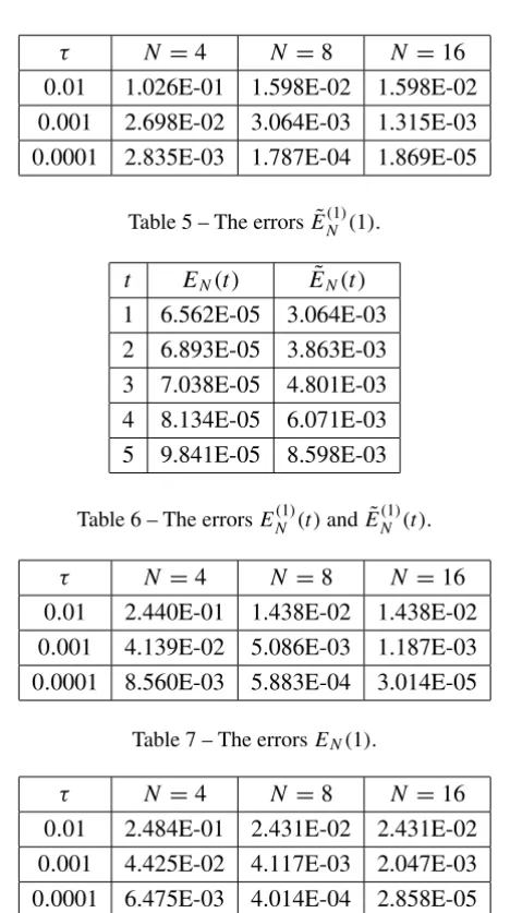
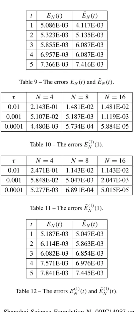
withb1 =b2 = 0.2 andh = 2.0. It decays algebraically and oscillates asx1 andx2tend to the infinity. We also use (3.6) and (4.1) to solve (3.5) numerically as before. The corresponding errorsEN(1)(t ) and E˜(N1)(t ) with various N and
t are presented in Tables 7-9 for (3.6) and Tables 10-12 for (4.1). They also demonstrate the high accuracy, the covergence and the stability of both schemes.
τ N =4 N =8 N =16
0.01 3.026E-03 2.074E-04 2.074E-04 0.001 4.799E-04 6.562E-05 3.862E-05 0.0001 5.469E-05 3.009E-06 2.724E-07
τ N =4 N =8 N =16 0.01 1.026E-01 1.598E-02 1.598E-02 0.001 2.698E-02 3.064E-03 1.315E-03 0.0001 2.835E-03 1.787E-04 1.869E-05
Table 5 – The errorsE˜N(1)(1). t EN(t ) E˜N(t ) 1 6.562E-05 3.064E-03 2 6.893E-05 3.863E-03 3 7.038E-05 4.801E-03 4 8.134E-05 6.071E-03 5 9.841E-05 8.598E-03
Table 6 – The errorsEN(1)(t )andE˜N(1)(t ).
τ N =4 N =8 N =16
0.01 2.440E-01 1.438E-02 1.438E-02 0.001 4.139E-02 5.086E-03 1.187E-03 0.0001 8.560E-03 5.883E-04 3.014E-05
Table 7 – The errorsEN(1).
τ N =4 N =8 N =16
0.01 2.484E-01 2.431E-02 2.431E-02 0.001 4.425E-02 4.117E-03 2.047E-03 0.0001 6.475E-03 4.014E-04 2.858E-05
Table 8 – The errorsE˜N(1).
6 Acknowledgment
t EN(t ) E˜N(t ) 1 5.086E-03 4.117E-03 2 5.323E-03 5.135E-03 3 5.855E-03 6.087E-03 4 6.957E-03 6.087E-03 5 7.366E-03 7.416E-03
Table 9 – The errorsEN(t )andE˜N(t ).
τ N =4 N =8 N =16
0.01 2.143E-01 1.481E-02 1.481E-02 0.001 5.107E-02 5.187E-03 1.119E-03 0.0001 4.480E-03 5.734E-04 5.884E-05
Table 10 – The errorsEN(1)(1).
τ N =4 N =8 N =16
0.01 2.471E-01 1.143E-02 1.143E-02 0.001 5.848E-02 5.047E-03 2.047E-03 0.0001 5.277E-03 6.891E-04 5.015E-05
Table 11 – The errorsE˜N(1)(1). t EN(t ) E˜N(t ) 1 5.187E-03 5.047E-03 2 6.114E-03 5.863E-03 3 6.082E-03 6.854E-03 4 7.571E-03 6.976E-03 5 7.841E-03 7.445E-03
Table 12 – The errorsEN(1)(t )andE˜N(1)(t ).
REFERENCES
[1] D. Gottlieb and S.A. Orszag,Numerical Analysis of Spectral Methods: Theory and Applica-tions, SIAM-CBMS, Philadelphia, (1977).
[2] Y. Maday, B. Pernaud-Thomas and H. Vandeven,One re´habilitation des méthods spectrales de type Laguerre, Rech. Ae´rospat.,6(1985), 353–379.
[3]O. Coulaud, D. Funaro and O. Kavian,Laguerre spectral approximation of elliptic problems in exterior domains, Comp. Mech. in Appl. Mech and Engi.,80(1990), 451–458.
[4] D. Funaro,Estimates of Laguerre spectral projectors in Sobolev spaces, inOrthogonal Poly-nomials and Their Applications, ed. by C. Brezinski, L. Gori and A. Ronveaux, Scientific Publishing Co., (1991), 263–266.
[5] Guo Ben-yu and Jie Shen,Laguerre-Galerkin method for nonlinear partial differential equa-tions on a semi-infinite interval, Numer. Math.,86(2000), 635–654.
[6] D. Funaro and O. Kavian,Approximation of some diffusion evolution equations in unbounded domains by Hermite functions, Math. Comp.,57(1990), 597–619.
[7] Guo Ben-yu,Error estimation for Hermite spectral method for nonlinear partial differential equations, Math. Comp., 68 (1999), 1067–1078.
[8] Guo Ben-yu and Xu Cheng-long,Hermite pseudospectral method for nonlinear partial dif-ferential equations, RAIRO Math. Mdel. and Numer. Anal.,34(2000), 859–872.
[9] R.A. Adams,Sobolev Spaces,Academic Press, New York, (1975).
[10] Guo Ben-yu,Spectral Methods and Their Applications,World Scientific, Singapore, (1998).
[11] Guo Ben-yu,A class of difference schemes of two-dimensional viscous fluid flow, TR. SUST, 1965, Also see Acta Math. Sinica,17(1974), 242–258.
[12] Guo Ben-yu,Generalized stability of discretization and its applications to numerical solution of nonlinear differential equations, Contemporary Math.,163(1994), 33–54.