M
ASTER
M
ONETARY AND
F
INANCIAL
E
CONOMICS
M
ASTER
´
S
F
INAL
W
ORK
D
ISSERTATION
B
ANKING
S
TABILITY
M
EASUREMENT AND
D
ETERMINANTS
:
E
VIDENCE
FROM
P
ORTUGAL
S
IMÃO
R
ODRIGUES
A
BREU
M
ASTER
M
ONETARY AND
F
INANCIAL
E
CONOMICS
M
ASTER
´
S
F
INAL
W
ORK
D
ISSERTATION
B
ANKING
S
TABILITY
M
EASUREMENT AND
D
ETERMINANTS
:
E
VIDENCE
FROM
P
ORTUGAL
S
IMÃO
R
ODRIGUES
A
BREU
S
UPERVISION:
MARIA TERESA MEDEIROS GARCIA
To my family and my girlfriend for their support and encouragement not only in the conception of this dissertation but also of my master journey.
i ABSI – Aggregate Banking Stability Index. AFSI – Aggregate Financial Stability Index AR – Autoregressive.
AT-1 – Additional Tier 1. BES – Banco Espírito Santo.
BSMD – Banking System’s Multivariate Density. CET-1 – Core Equity Tier 1.
CPI – Consumer Price Index.
CRD IV – Capital Requirements Directive. CRR – Capital Requirements Regulation. EBA – European Banking Authority.
EFAP – Economic and Financial Assistance Programme. EMEAP – Executives’ Meating of East Asia-Pacific. ESI – Economic Sentiment Indicator.
EWI – Early Warning Indicators. EWS – Early Warning Systems. FA – Factor Analysis.
FCI – Financial Conditions Index. FSI – Financial Soundness Indicators. GDP – Gross Domestic Product. HPI – House Prices Index.
IMF – International Monetary Fund. LCR – Liquidity Coverage Ratio.
ii NPL – Non-performing Loans.
NSFR – Net Stable Funding Ratio. OLS – Ordinary Least Square.
PCA – Principal Component Analysis. PD – Probability of Default.
PP – Percentage Point.
PSI20 – Portuguese Stock Index of the major 20 companies. RER42 – Real Exchange Rate with 42 trading partners. ROA – Return on Assets.
ROE – Return on Equity RWA – Risk-Weighted Assets.
SIP – Special Inspections Programme. VE – Variance-Equal.
iii
ABSTRACT,KEYWORDS AND JELCODES
A solid banking system is of key importance for the well-functioning of an economy, as it establishes a bridge between lenders and borrowers. Financial stability, particularly, banking stability, has been gaining a greater focus from supervisory authorities and academics due to its interconnectedness with the real economy. This dissertation aims to use a tool, the aggregate banking stability index (ABSI), to assess banking stability and its determinants in Portugal. In order to do so, firstly, an index reflecting banking stability during the 2010-2019 period is constructed. Secondly, with recourse to time series techniques, an analysis is made on the impact of macroprudential indicators, for the Portuguese banking system. Findings suggest for an improvement of the stability since 2017 and, in line with the empirical literature, point significant macroeconomic such as the growth rate of the consumer price index (%ΔCPI) and financial such as the ratio of the second money multiplier (M2) to gross domestic product (GDP) early warning indicators.
KEYWORDS: Banking System Stability; Time series Regression; Stability Index;
Financial Soundness Indicators; Macroprudential Indicators; Portugal.
iv
Glossary ... i
Abstract, Keywords and JEL Codes ... iii
Table of Contents... iv
List of Figures ... v
List of Tables ... v
Acknowledgments ... vi
1. Introduction ... 1
2. The Portuguese Banking Sector ... 2
3. Literature Review ... 4
3.1. Financial Stability Measures ... 4
3.2. Banking Stability Determinants ... 8
4. Aggregated Banking Stability Index ... 12
4.1. Deriving the ABSI ... 12
4.2. ABSI patterns ... 16
5. Aggregated Stability Determinants ... 20
5.1. Macroprudential Leading Indicators for the ABSI ... 20
5.2. Methodology ... 23
5.3. Results ... 25
6. Conclusion ... 28
References ... 30
v
FIGURE 1 – Total assets of monetary and financial institutions (MFI) in percentage of
Gross Domestic Product (GDP) in the 2000-2018 period for the Portuguese economy. . 3
FIGURE 2 – Portuguese ABSI and its average representation for the January 2010- January 2019 period. ... 16
FIGURE 3 – ABSI categories representation over time for the January 2010 – January 2019 period. ... 17
FIGURE 4 – Contributions of the categories in the ABSI time for the January 2010 – January 2019 period. ... 19
LIST OF TABLES TABLE I–SELECTED FSIS AND RESPECTIVE WEIGHTS AND IMPACTS ... 13
Table II – Description of the independent variables ... 21
Table III – Regression Output ... 25
TABLE A.I–CORE SET OF FSI FOR DEPOSIT TAKERS ... 35
Table A. II – ABSI data ... 36
TABLE A.III–WEIGHTED AND NORMALIZED CATEGORIES DATA ... 37
Table A. IV – Descriptive Statistics ... 38
Table A. V – Correlation matrix of the original variables... 39
Table A. VI – Correlation Matrix of the detrended and lagged variables ... 40
Table A. VII – Unit root tests results (ADF and PP) ... 41
Table A. VIII – p-values associated to the Chi-Square(l) of the Breusch-Godfrey serial correlation LM test ... 42
vi
First, I wish to thank Professor Maria Teresa Garcia for her encouragement and guidance during the elaboration of this dissertation. I wish to express my sincere gratefulness to Professor Isabel Proença for her prompt help on the empirical part of this dissertation.
Finally, I am also grateful to my girlfriend, Margarida, for her patience and support on numerous discussions during this demanding journey.
1
BANKING STABILITY MEASUREMENT AND DETERMINANTS: EVIDENCE FROM PORTUGAL
1. INTRODUCTION
The Great Recession highlighted the need of a cautious and precise assessment of the stability of the financial sector1, particularly, of the banking sector, which is the most preponderant component. Banks act, mainly, as liquidity intermediaries, i.e., they transform illiquid assets into liquid liabilities (Diamond & Dybvig, 1983). Thus, a solid banking system is required for a good allocation of capital and hence, for the well-functioning of the economy (Diamond, 1984).
Over the past decade, the maintenance of financial stability became, in addition to price stability, one of the main objectives of the Eurosystem,
Financial stability can be defined as a condition in which the financial system – which comprises financial intermediaries, markets and market infrastructures – is capable of withstanding shocks and the unravelling of financial imbalances. This mitigates the likelihood of disruptions in the financial intermediation process that are systemic, that is, severe enough to trigger a material contraction of real economic activity.
In European Central Bank (2019), p. 3. Furthermore, the banking system regulations have been suffering alterations across time. The Basel II, implemented in the course of 2007, relied in three pillars: minimum capital adequacy requirements, supervisory review process and market discipline (Basel Committee on Banking Supervision International, 2005). In response to the 2008 crisis, the Basel III agreement published in 2010, introduced more restrict minimum capital requirements, new composition of the Tier I equity (now subdivided into the common equity Tier I (CET-1) and the additional Tier I (AT-1)) and some new ratios (e.g. the Liquidity Coverage Ratio (LCR) and the Net Stable Funding Ratio (NSFR)) (Basel Committee on Banking Supervision International, 2010).
This dissertation aims to use a tool, the aggregate banking stability index (ABSI), to assess banking stability and its determinants in Portugal. In order to do so, firstly, an index
1 Which has been gaining greater influence in the economy. According to Haldane et al. (2010) the
“growth in the financial sector value added has been more than double that of the economy as a whole since 1850” in the U.K., similar trend were observed for the U.S. and Europe.
2
reflecting banking stability during the 2010-2019 period is constructed using data from the financial statements of the Portuguese banking system. Secondly, in an effort of assessing the interaction between the financial and the real sectors, an analysis is made on the impact of macroprudential indicators on the ABSI, classified into macroeconomic and financial variables, for the Portuguese banking system according with the empirical literature on early warning indicators (EWI) using time-series regressions.
The dissertation is structured as follows: the next chapter introduces the Portuguese banking sector. The third chapter reviews the body of literature dealing with the existing measures of financial stability and its determinants. The first section of chapter 4 presents the data used and its treatment for the construction of the aggregated banking stability index (ABSI), and the second section makes an analysis on its evolvement as well as on the contributions of each category in the analysed period. Chapter 5 is divided into three sections: the first deals with the choice of the candidates to be determinants of the banking stability, the second presents the methodology employed in the assessment of the ABSI determinants whereas the third section presents its results. Finally, chapter 6 summarize the conclusions of this dissertation.
2. THE PORTUGUESE BANKING SECTOR
Similarly, to Germany, Japan or France, Portugal is considered a bank-based economy whereas the United States and the United Kingdom are considered market-based economies.
In a bank-based financial structure, financing consists mostly of institutions that conduct financial intermediation on their balance sheet. These financial institutions bear risks and generally lend through close relationships with their clients. By contrast, a market-based financial structure primarily channels savings directly to borrowers through market.
3
FIGURE 1 – Total assets of monetary and financial institutions (MFI) in percentage of Gross Domestic Product (GDP) in the 2000-2018 period for the Portuguese economy.
Source: Eurostat
In Portugal, the banking sector is a central piece of the financial system. The plot in FIGURE 1 was achieved by making a ratio between two series (total assets of Portuguese
monetary and financial institutions and the Portuguese gross domestic product) from the Eurostat. As shown in FIGURE 1, the total assets of monetary and financial institutions
(MFI) in percentage of the gross domestic product (GDP) presented an increasing trend reaching its peak (307%) in 2012 and have been presenting a decreasing trend afterwards. Hence, the financial stability is highly dependent of the conditions of the banking sector which had a relatively good performance in the beginning of the century (Bank of Portugal, 2004). In 2006, the International Monetary Fund (IMF) carried out the Financial Sector Assessment Programme (FSAP). In their report, the IMF recognizes the solid Portuguese regulatory framework and the active and well-organized supervision of the Bank of Portugal. Furthermore, the results of the stress tests done on the Portuguese financial system allowed the IMF to conclude that the Portuguese banking system had shown an high resilience perceived as an adequate amount of capital to absorb extreme but plausible shocks (Bank of Portugal, 2006).
Nonetheless, the subprime crisis, in 2008, deteriorated the operational environment of the Portuguese banks. Mainly, by hindering their access to financing through the international debt markets and by lowering the value of their financial assets’ portfolio. In addition, the sovereign crisis in Portugal felt in the following years constrained the Portuguese banks’ liquidity even more.
150% 200% 250% 300% 350%
4
According to Bank of Portugal (2000, 2010, 2019) there were 43, 40 and 30 banks operating in January of 2000, 2010 and 2019, respectively, in Portugal.
The recent history of the Portuguese banking sector is marked by several negative events:
• In 2007, suspicions have fallen upon the Banco Comercial Português related with its activity causing a sharp decline on its shares price2.
• In 2008, the Banco Português de Negócios was nationalised. One month later, the Banco Privado Português required an injection of 450 million euros provided by a consortium of the main banking groups3.
• In 2014, the Bank of Portugal applied a resolution on Banco Espírito Santo (BES) (at the time the third largest bank in the system) giving origin to the Novo Banco, which kept a significant tranche of Banco Espírito Santo’s assets and liabilities4.
• In 2015, another resolution was applied on Banco Internacional do Funchal (the seventh largest bank in the system). Most of the bank’s assets and liabilities were sold to the Banco Santander Totta5.
3. LITERATURE REVIEW
Financial stability has been gaining more attention after the last global financial crisis, not only from the academics but also from central banks and other supervisory institutions. Among the body of literature, a greater focus is given to the measures of banking stability given the relevance of banking sector in the financial system. Section 3.1 reviews the financial stability measures whereas section 3.2 reviews the stability determinants literature.
3.1. Financial Stability Measures
Within the literature of financial stability measures many attempts were made on the construction of a stability index for the banking sector, which is the most relevant of the financial system. Whilst banking stability measures focus on the banking sector, financial
2 For more information, see box 4.1 (Bank of Portugal, 2007). 3 For more information, see box 4.1 (Bank of Portugal, 2008). 4 For more information see box 3 (Bank of Portugal, 2014). 5 For more information see box 2 (Bank of Portugal, 2016).
5
stability is a broader concept and considers the entire financial system. Although there is a wide body of literature on stability measurements, there is still no standard framework. There are several methodologies employable in the construction of an index, they vary in the variables used, the weighting procedure and in the complexity of the construction.
Gadanecz & Jayaram (2009) presented several attempts of researchers and pointed out the most commonly variables used to assess stability on six different sectors, their frequency and signalling properties as well as, what, indeed, they measure. Gadanecz & Jayaram (2009) also emphasize the importance of the individual indicators chosen in the construction of the composite indicator in order to capture different sources of fragility.
In an attempt to promote the international comparability and the standardization in concepts, definitions and techniques the IMF issued a compilation guide providing a list of a set of core and encouraged financial soundness indicators (FSI) (International Monetary Fund, 2006). The core set of indicators for deposit takers are related to five main areas compatible with the so-called CAMEL6 methodology.
The strand of literature dealing with EWI oftenly makes use of binary models. Nelson & Perli (2005) construct a logit model to identify periods of crisis using weekly data on twelve indicators which assigns the value 0 and 1 to non-crisis and crisis periods, respectively, using three summary statistics7 that contain the information of twelve individual indicators. However, as binary models assign the values 0 and 1 for non-crisis and crisis periods, they give less information about the developments of the economic conditions, which does not happen in the case of an index.
Goodhart & Segoviano (2009) conceptualize the banking system as a portfolio of banks and infer the banking system’s portfolio multivariate density (BSMD) from which the banking stability measures are constructed. Firstly, individual probabilities of default (PD) are calculated and used afterwards as exogenous variables in the consistent information multivariate density optimizing copula function (Segoviano, 2006) recovering the BSMD. The stability measures presented are intended to assess banking stability from three different but complementary perspectives: common distress in the
6 Where C stands for capital adequacy, A for asset quality, M for management soundness, E for
earnings and L for liquidity.
6
banks of the system, distress between specific banks and distress in the system associated with a specific bank. The fact that the PDs were used as exogenous variables provides flexibility to the model as PDs can be calculated using different approaches. Moreover, the BSMD captures linear and non-linear distress dependencies among banks in the system.
Van den End (2006) extends the so-called Monetary Conditions Index8 by adding house prices, stock prices, solvency buffer and the volatility of stock price index in terms of deviations from the trend. This measure captures the overall financial system as it includes not only indicators from the financial institutions’ balance sheets but also indicators from financial markets. The findings suggest that this index correctly reflects the boom/bust of the business cycle.
Jahn & Kick (2012) construct a forward-looking composite index for the German banking system comprising three components: the individual institutions’ scores (standardized PDs), the credit spread (the average bank risk premium) and a stock market index for the banking sector (prime banks performance index), where the first component is intended to capture the idiosyncratic risk whereas the latter two are intended to capture systemic risk. For major banks the individual institutions’ scores are derived from Moody’s Bank Financial Strength Ratings, whilst for small banks it is used the Bundesbank Hazard Rate Model. The framework consists in testing thirty-six combinations of weights using a partial proportional odds model using as a dependent variable the risk profile (A, B, C and D ranging from excellent grading to problem bank). Some literature uses higher frequency data (usually daily or weekly) from the financial markets (e.g. daily stock prices or exchange rates) for the construction of composite indices.
Illing & Liu (2006) use daily data of the Canadian banking sector, foreign exchange market, debt markets and equity markets to construct a financial stress index. Three different measure approaches are used, the standard measure, the refined measure and the generalized autoregressive conditional heteroscedasticity estimation techniques. These different measures are then combined using different weighting schemes. The authors
8 Monetary Conditions Index were previously developed by central banks to assess monetary policy
7
conclude that the standard-variable version allied with credit aggregate weighting technique produces the lowest type I and II errors9 and its components are simpler to interpret.
There is a trade-off in using higher frequency data. On one hand, the use of higher frequency data allows the rapidly assess of improvement/deterioration of the stability. On the other hand, higher frequency data tends to be more volatile, and hence, there is a possibility of yielding false signals to the decision makers (Kliesen et al, 2012).
Among the body of literature, the most common weighting techniques are the variance-equal (VE) and the factor analysis (FA). The former approach consists in standardize the individual indicators and assign them equal weights upon the construction of the index. Whereas the latter approach weights individual indicators based on their common variance, i.e. the more correlated an indicator is with its peers the greater the weight it receives. Both approaches have some shortcomings, the VE approach assumes normality of the variables and assumes that all the variables are equally important, and so, weights are meaningless in economic terms. Whereas the FA approach may generate multiple solutions (Puddu, 2013).
The most common methods of standardization are the statistical and empirical normalization. Statistical normalization produces normalized indicators ranging from -3 to 3 and is given by:
(1) Iitn=Iit-μi σi ,
where Iitn is the normalized value of the indicator i in period t, Iit is the value of the
indicator i in period t, μi and σi are the mean and standard deviation of the indicator i in the analysed period, respectively.
Empirical normalization produces normalized indicators ranging from 0 to 1 and is given by:
(2) Iitn=
Iit- min (Iit) max(Iit)- min (Iit),
9 Type I errors are the probability of failing to signal a crisis whereas Type II errors are the probability
8
where Iitn is the normalized value of the indicator i in period t, Iit is the value of the
indicator i in period t, min (Iit) and max(Iit) are the minimum and maximum value of the indicator i in the analysed period, respectively.
Both Albulescu (2010) and Cheang & Choy (2011) constructed an Aggregate Financial Stability Indicator for the Romanian and Macanese financial sectors, respectively, using the VE method and empirical normalization.
Both Kočišová (2016) and Gersl & Hermanek (2006) construct a banking stability index using the VE method to aggregate several FSI from the IMF core set, the former conducts a cross-country study on a yearly basis whereas the latter constructs only for the Czech banking sector.
Petrovska & Mihajlovska (2013) construct an ABSI and a financial conditions index (FCI) for Macedonia. The ABSI is a weighted sum of the indicators that represent the main risks faced by banks10. Individual indicators are normalized by the empirical normalization method and aggregated into their category according to their source of risk. The categories are weighted afterwards based on expert judgement. The FCI is constructed using the principal component analysis, the chosen threshold of 70% for the total common variance explained made the five principal components enough to summarize the data set. The resulting index is further divided by the share of total variance explained.
Dumičić (2016) constructs two indices for the Croatian financial system, one reflecting the accumulation of systemic risks and another reflecting its materialization, using the principal component analysis (PCA), whereas Hanschel & Monnin (2005) develop a stress index for the Swiss banking sector on an yearly basis using the VE as aggregation method.
3.2. Banking Stability Determinants
The empirical literature of banking stability determinants is quite large. The most common approaches are the signal extraction approach (non-parametric) and econometric approach (usually logit or probit models, which are parametric). Some studies use data on several countries where the crisis are represented by a binary variable (taking the value
9
1 in a crisis period and 0 otherwise) explaining them with explanatory variables (usually, macroeconomic) whereas some other just focus in assessing country-specific determinants.
Gaytán & Johnson (2002) present a survey of the literature in early warning systems (EWS) for financial crises. The authors state the importance of defining the scope and some concepts of the EWS. Firstly, it should be defined whether the EWS is aimed to assess individual bank failure or the entire banking system. Secondly, based on the scope selected, it should contain a precise definition of crisis or bank failure. Thirdly, a EWS requires a mechanism which includes a set of explanatory variables and the method to obtain the predictions from those variables. Gramlich et al. (2010) provide a critical review on the EWS literature and typology as well as a discussion on the principles to design an efficient EWS.
Kaminsky & Reinhart (1999) investigate the link between currency and banking crisis making use of the signal extraction approach for 20 economies in the 1970-1995 period. An indicator signals a crisis/distress if the value of such indicator exceeds its threshold value. If the crisis/distress does happen in the following 12 months, then the signal is considered a good signal, otherwise it is a false alarm. The threshold value is chosen to minimize a noise-to-signal ratio. Based on this ratio, the three best indicators are the real exchange rates, stock prices and the ratio of public sector deficit to GDP.
Borio & Lowe (2002a) also use the signal extraction approach, however, instead of individual indicators they use composite indicators which improves the predictive power in their sample. Their results point that for industrial countries the best composite indicator combines the credit gap with the equity price gap. Whereas for emerging market countries the best composite indicator is the credit gap with either the asset price gap or the exchange rate gap. Their results were further confirmed by Borio & Drehmann (2009) concluding that, besides the credit-to-GDP ratio, the asset prices and the gross fixed investment, the property prices have also a strong predictive power on banking crisis.
Using the signal extraction approach, Christensen & Li (2014) construct three composite indicators – the summed composite, the extreme composite and the weighted
10
composite – from 12 individual indicators11 for 13 OECD countries. Their in-sample forecasting results suggest that the three composite indicators are useful tools to predict crisis. However, their out-of-sample forecasting results suggest that the weighted composite indicator outperforms the other two composite indicators.
Misina & Tkacz (2009) use the financial stress index developed by Illing & Liu (2006) in order to assess the possibility of the credit and asset prices movements helping to predict financial stress in the Canadian economy. Their finddings suggest that housing prices and business credit provide the lowest forecast errors in a 2-year horizon for the Canadian economy.
Demirgüç-Kunt & Detragiache (1998) apply a multivariate logit approach to assess the probability of the occurrence of a crisis through a set of explanatory variables which showed that economic growth, inflation and real interest rates have a strong impact on the probability of a banking crisis. In a posterior paper, Demirgüç-Kunt & Detragiache (2005) compare the two most common approaches, suggesting the prominence in the suitability of the logit model approach. Hardy & Pazarbaşioğlu (1999) use a multivariate-multinomial logit model and, define a discrete variable that takes the value of 1 in the year that precedes the crisis, the value of 2 in the year of the crisis, and zero otherwise. In contrast with Demirgüç-Kunt & Detragiache (1998), they also include lags of the explanatory variables allowing a dynamic analysis of the variables.
Hutchison & McDill (1999) estimate a multivariate probit model to assess the relationship of banking problems with a set of macroeconomic (real GDP growth, real credit growth, nominal and real interest rate increase, inflation, the change in an index of stock prices, the M2-to-reserves ratio and exchange rate depreciation) and institutional variables (explicit deposit insurance, financial liberalization, moral hazard and central bank independence). Their results point the best model to be the one with all the macroeconomic and institutional variables except for the stock prices index.
Wong et al. (2007) develop a probit econometric model to identify leading indicators of banking distress for Hong Kong and other Executives’ Meating of East Asia-Pacific (EMEAP) economies. Their fiddings suggest that GDP growth, inflation, increase in
11 Most of the indicators were extracted from Demirgüç-Kunt & Detragiache (1998), Kaminsky (1999)
11
money supply relative to foreign reserves, asset prices along with strong credit growth are good leading indicators of banking distress.
Pereira Pedro et al. (2018) assess the main determinants of banking stability from three different perspectives – bank-specific determinants, country-specific macroeconomic determinants and whether regulation and supervision prevent banking crisis. At the macroeconomic level they found that the GDP growth and the inflation rate affects the probability of having a banking crisis and that real GDP growth is the most robust indicator in contrast with the GDP per capita, which showed to be irrelevant to explain banking crisis.
Lainà et al. (2015) assess 19 potential leading indicators of systemic banking crises in Europe, giving special attention to the Finnish case and making use of the two most common methods. The results of the signal extraction approach suggest the prominence of the growth rates vis-à-vis trend deviations. Namely, the growth of OECD loans-to-deposits ratio, the growth of real private loans, the real GDP growth, the real house prices growth, real households’ loans growth and real private loans growth which have presented a noise-to-signal ratio less than 30%. The multivariate logit regressions suggest that deviations from the trend are better explanatory variables for shorter term horizons (e.g. 1-year lagged variables). The real house price growth, real GDP growth, mortgage stock growth, private loan stock growth and household loan stock growth are appropriate crisis indicators.
Following Betz et al. (2014) and Black et al. (2016), Shijaku (2016) assesses the banking stability determinants by estimating a benchmark model through means of a panel ordinary least square (OLS) approach. The dependant variable is the stability indicator explained by three sets of variables – a set of banking-specific variables, a set of industry-specific variables and a set of macroeconomic variables. In what concerns to the macroeconomic variables, the GDP showed to improve banking stability and to be statistically significant at 1% level whereas the spread between Albanian and German 12-month T-bills deteriorates banking stability, but it turned out to be statistically insignificant.
Using the gap approach developed by Borio & Lowe (2002b), Hanschel & Monnin (2005) assess the determinants of the stress index by taking the index as the dependent
12
variable of the regression and using as explanatory variables (comprised between 1 and 4-year lag) the GDP gap, the European GDP gap, the share price index gap, the housing price index gap, the credit ratio gap and the investment ratio gap.
The second part of Jahn & Kick (2012) focus on assessing the determinants of the German banking stability with 3 macroeconomic variables (real estate price index, ifo index12 and gross fixed investments), 3 financial variables (national private credit-to-GDP ratio, 3-month libor, and M2-to-GDP ratio) and 5 structural variables (regional probability of default, regional GDP change rate, international exposures, risk aversion and an indicator representing the bank size). Making use of a dynamic panel data model, they found that in contrast with the gross fixed investments, the real estate price index and ifo index are leading macroprudential indicators for banking stability. Furthermore, within the financial variables, the 3-month libor and the national private credit-to-GDP are good banking stability indicators (however, the latter becomes less important for internationally oriented banks). Finally, the regional probability of default and regional GDP change are significant determinants only for small cooperative banks, whereas the risk aversion indicator showed to be a prominent banking stability determinant.
4. AGGREGATED BANKING STABILITY INDEX
4.1. Deriving the ABSI
TABLE A.I (appendix) summarizes the core set of FSI provided by the IMF. Most of them consist in a ratio between two underlying series. They rely on five main categories relevant from the banking business perspective and provide insights about the banking system position, as the data is obtained through the banks’ financial statements. Some indicators from the core set FSI were not included in the ABSI calculation. The two Basel III indicators, the LCR and the NSFR, were excluded. As they are quite recent, these two concepts are still in implementation. Contrasting with the LCR, the NFSR does not have a compulsory disclosure yet, having no available data. The introduction of the LCR on the ABSI construction would require a break in the series causing a major reduction in the time window under analysis. The net open position in foreign exchange to capital and residential real estate prices were also excluded due to the lack of available data.
12 The Ifo index is an index developed by the Ifo institute for Economic Research, that measures
13
The ABSI constructed in this dissertation uses selected quantitative indicators of the core set of FSI of the IMF with its calculation being tested from March 31, 2010 to March 31, 2019, on a quarterly basis. The data for the FSIs was obtained from the Bank of Portugal database, the BPstat.
TABLE I–SELECTED FSIS AND RESPECTIVE WEIGHTS AND IMPACTS
Category Weight Indicator Impact Data
Source
Capital Adequacy 0.25
Regulatory capital to
risk-weighted assets. + BPstat
Regulatory Tier 1 capital to risk-weighted
assets.
+ BPstat
CET-1 capital to
risk-weighted assets. + BPstat
Nonperforming loans net of provisions to
capital.
- BPstat
Tier-1 capital to assets. + BPstat
Asset Quality 0.25
Nonperforming loans to
total gross loans. - BPstat
Sectoral distribution of
loans to total loans. - BPstat
Provisions to
nonperforming loans. + BPstat
Earnings and
Profitability 0.25
Return on assets. + BPstat
Return on equity. + BPstat
Interest margin to gross
income. + BPstat
Noninterest expenses to
gross income. - BPstat
Liquidity 0.25
Liquid assets to total
assets + BPstat
Liquid assets to
short-term liabilities + BPstat
14
TABLE I presents the set of indicators used on the ABSI construction. The ABSI
proposed, is subdivided into four main categories. These categories represent the main sources of risk for the banks.
Capital adequacy ratios are the central feature of the Basel Capital Accord. It represents the insolvency risk and shows the banks’ capacity to deal with potential risks, measuring the banks’ capital buffer to absorb expected or unexpected losses. The first is a ratio where the numerator is the total regulatory capital (supervisory definition of capital developed by the Basel Committee on Banking Supervision) and the denominator is the on and off-balance-sheet assets weighted by risk. Therefore, an increase in this ratio is expected to lead to a more stable banking system. The second focuses on a more specific concept of capital, the Tier 1, measuring the most freely and readily available resources to absorb losses. The third is an even more restrict definition of capital, it measures the banks’ capital adequacy based on the highest-quality capital, the CET-1. Both the second and the third ratios impact stability in the same way as the first as they are just more restrict concepts than the first. The fourth FSI is intended to capture the impact of the non-performing loans (NPL) not covered by specific provisions on capital, where the numerator is the difference between the NPL and the specific provisions and the denominator is the regulatory capital. An increase in this ratio reflects a lower capacity of the banks’ capital to withstand NPL losses and so it impacts stability negatively. The last capital adequacy FSI is a proxy for financial leverage, i.e., it indicates in which extent the amount of assets is funded by other than own funds. Thus, an increase in this ratio reflects a lower exposure to risk, hence affecting banking stability positively.
The asset quality ratios are intended to capture the credit risk, it is assessed through three indicators. The first ratio is the proportion of NPL in the total gross loans, it reflects the proportion of troubled loans in the total gross loans. An increase in this ratio implies a poorer quality of the credit granted, impacting negatively the banking stability. The sectoral distribution of loans to total loans ratio consists in taking the credit granted to the three largest economic activities as the numerator and the total gross loans as the denominator. It reflects the concentration of the credit granted, an excessive concentration of the loans implies a higher exposure to fewer activities (less diversified loan portfolios) and so an increase in this ratio affects negatively banking stability. The last asset quality ratio measures the amount of NPL that are already covered by specific provisions and
15
provides information about future losses if all NPL were written-off. Thus, an increase in this ratio implies a more stable banking system.
There are four FSI for the earnings and profitability category. The return on assets (ROA) is a ratio of the net income and the average total assets and provides an insight on the banks’ efficiency in managing their assets to generate earnings. The return on equity (ROE) is a ratio of the net income and the average book equity and provides an insight on the banks’ efficiency in using their capital to generate earnings. These two FSI are expected to affect stability positively. The interest margin to gross income is the share of the interest margin within gross income, it reflects the relative importance of intermediation business. The noninterest expenses to gross income ratio, also called efficiency ratio, is the portion of revenues required to off-set operating expenses.
Liquidity management is one of the main concerns (and source of risk) on the banks’ activity, i.e., the banks’ ability to meet cash outflows. The liquid assets (assets that can be converted into cash with low haircut) to total assets ratio measure the available term liquidity. The liquid assets to term liabilities measures the portion of short-term liabilities covered by liquid assets. Both FSIs have a positive impact on banking stability.
Before the final aggregation, the data passed through an adjustment process. Firstly, since this ABSI focus on measuring the banking stability, those FSIs which have a negative impact on the ABSI (i.e., sources of instability) need to be adjusted in order to have a positive impact. Thus, their reciprocal value is taken (e.g.: 1 − 𝑁𝑃𝐿
𝑅𝑒𝑔𝑢𝑙𝑎𝑡𝑜𝑟𝑦 𝐶𝑎𝑝𝑖𝑡𝑎𝑙).
In a second phase, all FSIs were normalized to have the same variance through the empirical normalization method presented in Equation (1). In this way, each indicator is compared to its limit values (minimum and maximum) in the analysed period. Movements of the ABSI towards 0 (the lower limit) means larger risk exposure whereas movements towards 1 (the upper limit) means lower risk. On one hand, since this method uses the limit values for the adjustment, it can be unreliable for entire data series. On the other hand, minor date-to-date changes leads to obvious effects on the ABSI. Moreover, the fact that this method comprises indicators in the interval from 0 to 1 provides an easy interpretation of the ABSI developments. The third step of the ABSI calculation consisted in calculating, for every quarters, each category by taking the arithmetic mean of the FSIs
16
that compose it. Finally, given that there are four categories and that variance-equal scheme was used, it was allocated a weight of 25% to each category. The ABSI is then, a weighted sum of the values of the four categories.
4.2. ABSI patterns
The ABSI is calculated as a weighted sum of the adjusted and normalized components of the four categories. As mentioned in the previous section, an increase in the ABSI value corresponds to an increase of the stability in that period.
FIGURE 2 – Portuguese ABSI and its average representation for the January 2010- January 2019 period.
FIGURE 2 shows the ABSI development and its average of the Portuguese banking system stability13 for the analysed period. The ABSI was constructed on a quarterly basis from the first quarter of 2010 until the first quarter of 2019, presenting an average value for the entire analysed period of 0.51019. The analysed period can be divided into three stages:
• The first stage covers the period from the first quarter of 2010 until the second quarter of 2012. Even though the ABSI is above its average value (with the fourth quarter of 2011 as an exception), it presented a downward trend. • Despite the first two quarters of 2015, where the ABSI stood barely above its
average value, the second stage can be identified from the third quarter of 2012 until late 2016, where the ABSI presented lower values when compared to its mean, reaching its minimum of 0.33041 in the second quarter of 2014.
17
• The third stage covers the final period from early 2017 until the end. This stage is characterized by an upward trend in stability, reaching its peak of 0.79402 in its final value.
FIGURE 3 – ABSI categories representation over time for the January 2010 – January
2019 period.
FIGURE 3 shows the evolvements of the ABSI categories during the period under
analysis14. On one hand, the capital adequacy was the category that presented the most remarkable improvement over time, increasing from 0.05901 in the first quarter of 2010 to 0.23999 in the first quarter of 2019. On the other hand, the liquidity category was the one that presented the poorest behaviour, decreasing its contribution from 0.15656 to 0.13637. Both the asset quality and earnings and profitability categories presented some improvements, the former increased from 0.16279 to 0.20548 whereas the latter increased from 0.17822 to 0.21218.
During the first stage the improvements of the capital adequacy category were due to the more strict capital requirements ratios defined on the basis of the Economic and Financial Assistance Programme (EFAP), the deleveraging process undertaken by the Portuguese banks reducing their risk-weighted assets and the capitalizations required by the European Banking Authority (EBA) on the four major banks (Bank of Portugal, 2014). The upward trend in capital adequacy ratios remained in 2013, due to the decline of the risk-weighted assets (RWA) and the banks’ recapitalization with recourse to public
14 For specific values of the ABSI, see TABLE A.III–WEIGHTED AND NORMALIZED CATEGORIES DATA
18
funds. The resolution made on BES influenced negatively the capital adequacy ratios causing the deterioration verified in 2014. Up to 2016 the negative developments on this category were due to the weak profitability and the progressive elimination of the transitional provisions established in the Capital Requirements Regulation (CRR) and Capital Requirements Directive (CRD IV) that were partially offset by the continuing decline in the RWA. The good evolvement of capital adequacy ratios since 2016 were due to the positive development in the banks’ profitability (allowing internal generation of capital), the continuous downward trend of the RWA resulted from the deleveraging process and recapitalization processes carried out through several banks in the system.
The credit quality presented a negative trend during the first stage. This degradation reflected the increase in the default ratios on loans either to households or to non-financial companies, due to the worsening of the macroeconomic scenario: in the case of the households the rise in the unemployment and fiscal burden and the decrease on wages were the main factors, whereas in the case of the non-financial companies the contraction of the domestic demand limited, severely, the generation of resources. The developments on the asset quality were marked by the continuous deleveraging process and the consequent reduction on the banks’ assets and by the increase in the credit at risk. The non-financial sector reached its highest credit at risk ratio at the end of 2015 impacting negatively this category. The improvements felt in this category afterwards, were a result from continuous decrease in the stock NPL (resulted from a high flow of loan write-offs and the better performance non-financial companies whose share of NPL started to decrease) and the strengthening of impairment recognition (verified by the increase in the coverage ratio of NPL’s by provisions).
A set of non-recurring events in 2011, such as the Special Inspections Programme (SIP) that highlighted the need to reinforce the recognition of impairment losses and provisions, along with the decrease in financial operations’ income led to a sharp decrease in the Portuguese banks’ profitability. Part of the recovery felt in 2012 is, then, due to cease of those non-recurring events and the slight improvement of both the operating costs and income from financial operations. The profitability of Portuguese banks continued to fall, highly influenced by the impairments’ costs and the contraction on the net interest margin even with the positive contributes of the decrease in the operation costs and the income from financial operations. The profitability of the Portuguese
19
banking system was negatively influenced by the resolution applied on BES, during the first half of 2014. Nonetheless, this marked a turning point in the profitability, that present a positive trend afterwards. 2015 was marked by the return to positive levels of the profitability (that were not verified since 2010) (Bank of Portugal, 2015). For this positive development contributed the rise in net interest income (through the reduction of interest expenses), the continued positive results of financial operations and a reduction in the flow of impairments’ costs and a continued downward trend in banks’ operational costs. The hindered access to wholesale debt markets15 in 2010 implied a reduction of long-term bonds financing, compelling Portuguese banks to adjust their financing strategy by increase their reliance on Eurosystem lending operations and to attract stable deposits (over 2-year maturity, e.g., savings deposits). Despite the long-term refinancing operations carried out by the European Central Bank (ECB), 2012 was marked by a significant increase in subordinated liabilities due to the issues of contingent capital instruments subscribed by the Portuguese state associated with the capitalization needs deriving from stricter capital regulations (Bank of Portugal, 2012).
FIGURE 4 – Contributions of the categories in the ABSI time for the January 2010 – January 2019 period.
FIGURE 4 displays the contributions of each category16 for the ABSI in each and every
quarter of the analysed period. Although it is a combination of the information of the two previous figures, it provides a better intuition about the contribution of each category to
15 This restriction was highly influenced by the sovereign debt crisis.
16 For specific values of the ABSI, see TABLE A.III–WEIGHTED AND NORMALIZED CATEGORIES DATA
20
the ABSI. During the first stage, the main contributors to the maintenance of the ABSI above the average were the liquidity along with the earnings and profitability. The beginning of the second stage coincides with the sharp fall in the contribution of the liquidity category that pushed the ABSI below the average even with the increase in the contribution of the capital adequacy. In addition to the sharp fall in the liquidity contribution, the decreasing contribution of the earnings and profitability pushed the ABSI further below, reaching its minimum in the second quarter of 2014. The rest of the second stage was influenced by opposite trajectories of the earnings and profitability (which showed an improvement) and the asset quality (which showed a deterioration). The third stage is characterized by a good performance of all categories imposing a quite stable improvement on the ABSI, reaching its peak in the end-period.
5. AGGREGATED STABILITY DETERMINANTS
5.1. Macroprudential Leading Indicators for the ABSI
The empirical work of this dissertation began with the construction of an index reflecting the aggregated banking stability index (the ABSI), which will now be used as the dependent variable to assess the determinants of the Portuguese banking stability.
Descriptive statistics of all the variables (dependent and independent) used are presented in Table A. IV (appendix).
Regarding the dependent variable, this assessment includes 37 observations from the first quarter of 2010 through the first quarter of 2019. Based on the related theoretical and empirical literature several indicators were identified as potential candidates to be determinants of the Portuguese aggregate banking stability and classified into macroeconomic and financial variables.
21
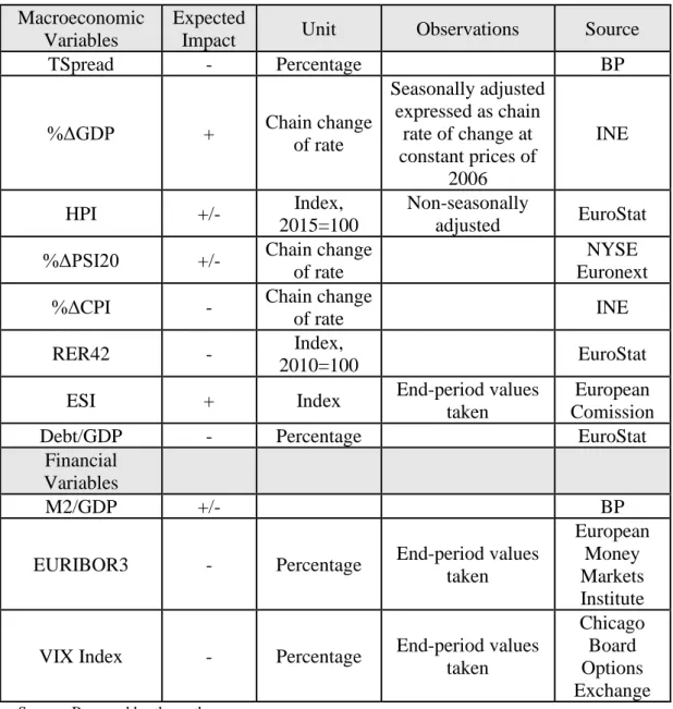
TABLE II–DESCRIPTION OF THE INDEPENDENT VARIABLES
Macroeconomic Variables
Expected
Impact Unit Observations Source
TSpread - Percentage BP %ΔGDP + Chain change of rate Seasonally adjusted expressed as chain rate of change at constant prices of 2006 INE HPI +/- Index, 2015=100 Non-seasonally adjusted EuroStat
%ΔPSI20 +/- Chain change
of rate
NYSE Euronext
%ΔCPI - Chain change
of rate INE
RER42 - Index,
2010=100 EuroStat
ESI + Index End-period values
taken
European Comission
Debt/GDP - Percentage EuroStat
Financial Variables
M2/GDP +/- BP
EURIBOR3 - Percentage End-period values
taken
European Money Markets Institute
VIX Index - Percentage End-period values
taken
Chicago Board Options Exchange
Source: Prepared by the author.
Table II presents the units and sources of the data of the independent variables, as well as the specifications under which each one was calculated and their expected impact on the ABSI.
The set of macroeconomic variables comprises eight variables that reflect the conditions of the Portuguese economy:
• The spread between domestic and German 10-year government bonds (TSPREAD) reflects the risk premium associated with the Portuguese government debt when compared to the safest European debt, the German.
22
The high indebtedness of the Portuguese state during the financial crisis hindered the access of Portuguese banks to wholesale debt markets. Thus, an increase in the spread is expected to harm stability, as it indicates a riskier Portuguese public debt relative to the German debt.
• The government debt-to-GDP ratio (Debt/GDP) compares what the country owes with what the country produces on a given date. Typically, higher debt-to-GDP ratio is associated to higher risks, since it would take more time to repay its debt without further refinancing. Thus, this regressor is expected to have a negative impact on stability.
• The real GDP growth (%ΔGDP) is the main macroeconomic indicator, a positive value indicates an expansion period whereas a negative value is associated to a recession and a slowdown of the economy. Thus, this indicator is expected to have a positive impact on banking stability.
• Theoretically, positive asset prices growth is associated with the boom phase in the business cycle. However, large growth rates might signal the overheating of the economy and hence, future instability. Within asset prices, here they are distinguished between two types: property prices represented by the house price index (HPI) and stock prices represented by Portuguese stock index of the twenty major companies (PSI20). Real estate prices played an important role in the last financial crisis since the crisis emerged after the bust of the real estate bubble.
• The variation in consumer price index (%ΔCPI) is intended to proxy inflation. Thus, a positive variation in the CPI is associated with positive inflation. High inflation rates are usually seen as source of instability and its increase may lead to a contraction of the international demand for domestic products (Hoggarth et al. 2005). Thus, its estimated coefficient is expected to be negative.
• The real exchange rate with 42 trading partners (RER42) reflects the international competitiveness. Thus, an increase in the real exchange rates reflects a deterioration in competitiveness and so, is expected to have a negative estimated coefficient.
23
• The economic sentiment indicator (ESI) measures the confidence or expectations of economic agents. So, an increase in this index reflects improvements of the agents’ expectations. Thus, it is expected to have a positive impact on stability.
The set of financial variables comprises three variables:
• The M2-to-GDP is a ratio where the numerator (M2) is a measure of the money supply that includes M1 (cash and checking deposits) as well as savings deposits money market securities, mutual funds and other time deposits and the denominator is the GDP. It is a proxy for financial depth, also reflecting the excessive liquidity that might precede a lending boom. • The 3-month euro interbank offered rate (EURIBOR3) is the average interest
rate at which banks borrow funds for 3-month maturity from one another. If the financial environment is weak, then 3-month Euribor should be high. Hence, an increase of the Euribor is expected to decrease stability and so, its coefficient is expected to be negative.
• The volatility index (VIX index) is intended to proxy risk-aversion and uncertainty in financial markets (Bekaert et al., 2013). Thus, it is expected to have a negative impact on stability.
The correlation matrix of the original variables is presented in Table A. V (appendix) whereas the correlation matrix for the detrended variables with the respective lags is presented in Table A. VI.
5.2. Methodology
Many economic and financial time series exhibit non-stationarity properties resulting in spurious regressions. Therefore, before any estimation, it is necessary to check the stationarity of the series in use through both the Augmented Dickey-Fuller and Phillips-Perron unit root tests, see Table A. VII (appendix). The unit root tests the null hypothesis that the series has a unit root (i.e. is non-stationary). This procedure consisted in testing all variables in level and differentiate those that failed to reject the null hypothesis until they do (at a minimum of significance level of 10%). Thus, some variables enter the model in levels, some enter in the first difference and some in the second difference.
24
To conduct the empirical study ARMA conditional least squares was used17, of the following regressions: (3) Yt= β0+ ∑Jj=1 jβ ∙Xj,t-p+ ∑Kk=1 kβ ∙Zk,t-q+ εt, with t = 1, 2, …, 37; j =1, 2, …, 8 and k = 1, 2, 3. (4) Yt= β0+ ∑Jj=1 jβ ∙Xj,t-p+ ∑Kk=1 kβ ∙Zk,t-q+ εt+ar(1) , with t = 1, 2, …, 37; j =1, 2, …, 8 and k = 1, 2, 3. (5) Yt= β0+ ∑Jj=1 jβ ∙Xj,t-p+ ∑Kk=1 kβ ∙Zk,t-q+ εt+ar(1)+ar(2), with t = 1, 2, …, 37; j =1, 2, …, 8 and k = 1, 2, 3. (6) Yt= β0+ ∑Jj=1 jβ ∙Xj,t-p+ ∑Kk=1 kβ ∙Zk,t-q+ εt+ar(1)+ar(2)+ar(3), with t = 1, 2, …, 37; j =1, 2, …, 8 and k = 1, 2, 3.
These econometric relationships involve the dependent variable (𝑌𝑡), which is the ABSI calculated in section 4.1; 𝛽0, the constant term; X and Z the explanatory variables; 𝜀𝑡, the disturbance term; 𝑎𝑟(1), 𝑎𝑟(2) and 𝑎𝑟(3), the autoregressive components.
The term ∑𝐽𝑗=1𝛽
𝑗∙ 𝑋𝑗,𝑡−𝑝 corresponds to macroeconomic variables whereas,
∑𝐾𝑘=1𝛽𝑘∙ 𝑍𝑘,𝑡−𝑞 corresponds to the financial variables. The lags are allowed to differ across the regressors. The coefficients 𝛽𝑗 and 𝛽𝑘 describe the effect of 𝑋𝑗,𝑡−𝑝 and 𝑍𝑘,𝑡−𝑞 on 𝑌𝑡 and are constant across time.
When using time series, the most serious problem that can arise regards the serial correlation. So, it is important to check for serial correlation in the error terms upon every estimation of the model. E-views tests the null hypothesis of no serial correlation through the Breusch-Godfrey Serial Correlation LM test for different lag lengths. Since we are dealing with quarterly data, the test was undertaken for 1, 2 and 4 lags, the results are presented in Table A. VIII (appendix). The model in equation (3) failed to reject the null hypothesis of no serial correlation since it presented a p-value<0.05. However, e-views enables to address this problem by adding an autoregressive (AR) component to the equation. The models in equation (4) and (5) also failed to reject the null hypothesis,
17 For equation (3) the estimation method used was the ordinary least squares. The ARMA conditional
25
indicating that 𝑎𝑟(1) and 𝑎𝑟(2) are not a good specification, as they do not fully address serial correlation. The model in equation (6) rejects the null hypothesis of no serial correlation, indicating that an autoregressive process of order 3 addressed properly the problem of serial correlation.
Heteroskedasticity problems can also arise in time series, especially in small samples. E-views allows to test for heteroskedasticity through several tests. In this dissertation it was used the White test and the Breusch-Pagan-Godfrey test. Both test the null hypothesis of homoskedasticity, and both results point to the presence of homoscedastic errors. The heteroskedasticity test results are presented in Table A. IX (appendix).
5.3. Results
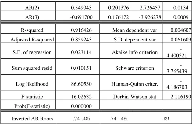
TABLE III–REGRESSION OUTPUT
Dependent Variable: D1_ABSI
Method: ARMA Conditional Least Squares (Gauss-Newton / Marquardt steps)
Sample (adjusted): 2011Q1 2019Q1
Included observations: 33 after adjustments Convergence achieved after 14 iterations
Coefficient covariance computed using outer product of gradients
Variable Coefficient Std. Error t-Statistic Prob.
C 0.049615 0.014180 3.498925 0.0024 D1_TSPREAD (-1) 0.049616 0.005056 9.812958 0.0000 D2_DEBT/GDP(-3) 0.004734 0.000641 7.388061 0.0000 %ΔGDP (-2) -0.033503 0.007947 -4.215941 0.0005 D1_%ΔCPI (-2) -2.161260 0.472075 -4.578217 0.0002 D2_HPI(-2) -0.014286 0.001968 -7.259308 0.0000 %ΔPSI20(-2) 0.002219 0.000724 3.063831 0.0064 D1_ESI(-1) 0.010183 0.001542 6.603718 0.0000 D1_M2/GDP(-2) 0.143626 0.057144 2.513408 0.0211 EURIBOR3(-1) -0.060762 0.017200 -3.532729 0.0022 VIX_INDEX -0.001797 0.000626 -2.867670 0.0099 AR(1) 0.584938 0.178272 3.281154 0.0039
26
AR(2) 0.549043 0.201376 2.726457 0.0134
AR(3) -0.691700 0.176172 -3.926278 0.0009
R-squared 0.916426 Mean dependent var 0.004607
Adjusted R-squared 0.859243 S.D. dependent var 0.061609
S.E. of regression 0.023114 Akaike info criterion
-4.400321
Sum squared resid 0.010151 Schwarz criterion
-3.765439
Log likelihood 86.60530 Hannan-Quinn criter.
-4.186703
F-statistic 16.02632 Durbin-Watson stat 2.116190
Prob(F-statistic) 0.000000
Inverted AR Roots .74-.48i .74+.48i -.89
Source: E-views 9.0 estimation results.
Notes: D1 and D2 indicate whether the variable enters in the first or second difference, respectively.
Table III reports the estimation of the model for the analysed period (2010-2019). The main results point that most of the macroprudential indicators commonly used in the literature to predict banking crisis or instability, are also useful leading indicators for Portugal. Overall, the model presents a strong explanatory variable, as the R-squared is approximately 92% and all the regressors showed to be statistically significant at 1%, with exception for the M2/GDP coefficient which is significant at 5% level. Within the set of potential determinants of stability, RER42 was the only candidate that showed to be not statistically significant. Thus, it was removed from the model.
The coefficients of both the TSPREAD and the DEBT/GDP showed a positive impact (although they were expected to be negative) on the ABSI growth, indicating that an increase of 1 percentage point (PP) on the TSPREAD growth increases the ABSI growth in the subsequent period by 0.049615PP, whereas an increase of 1 unit on the variation of DEBT/GDP growth increases the ABSI growth by 0.004734PP after three quarters. One possible reason for the unexpected sign of the coefficients, could lie in the fact that the Portuguese government undertook several measures (e.g. bailouts and capital injections in the banking system) to avoid major distresses in the banking system. Likewise, it was possible to have an increase in government debt and yields affecting
27
positively banking stability. Conversely, the coefficient of the %ΔGDP presents a negative sign (contrary to what was expected) indicating that an increase of 1pp of %ΔGDP decreases the ABSI growth by 0.033503PP two periods after. One reason for this, might be the low average growth rate (0.09%) allied with a negative skewness18 that the Portuguese economy experienced in the analysed period. Thus, the stability of the Portuguese banking system could have benefited from higher GDP growth rates. The negative coefficient of %ΔCPI reflects that an increase of 1 unit in the variation of %ΔCPI decreases the growth of the ABSI by 2.161260PP after two quarters. The coefficient of the HPI shows that an increase of 1 unit in the variation of the HPI growth impacts the ABSI growth by -0.014286PP in the following two periods. %ΔPSI20 presents a positive coefficient reflecting that an increase 1PP in the %ΔPSI20 impacts the ABSI growth by 0.002219PP in the two following periods. As expected, the coefficient of the ESI presents a positive sign, indicating that an increase of 1 unit in the ESI growth impacts the growth of the ABSI by 0.010183PP in the subsequent period.
Turning to financial variables, the M2/GDP presents a positive sign, indicating that an increase of 1 unit in the M2/GDP growth impacts the ABSI growth by 0.143626PP. The negative coefficient of the EURIBOR3, as expected, indicates that an increase of 1pp in this interest rate affects negatively the ABSI growth in the subsequent period by 0.060762PP. The VIX index presented a negative coefficient, as expected, indicating that an increase of 1 unit contemporaneously affects the ABSI growth by 0.001797PP.
Finally, the level of significance associated with the coefficients of the AR terms show that the model properly addresses the problem of serial correlation in the disturbance terms.
18 A negative skewness indicates a left-sided tail which means a larger number of observations below
28 6. CONCLUSION
Over the recent past, the Portuguese banking system have been exhibiting some difficulties, namely, after the last global financial crisis. Furthermore, there is a continuous improvement in the regulatory and supervisory system (e.g. more strict ratios, new concepts such as the LCR and NSFR), which obliges banks to perform in a constantly changing environment. Banks are central players in the financial system and play a very important role in the financing of the economy. Thus, it is very important to surveil the banking system stability in order to maintain prosperous conditions to the economy as whole.
The main goal of this dissertation is, then, to assess the stability of the Portuguese banking system and to assess whether the common macroprudential leading indicators can be also used as determinants for the Portuguese case. Therefore, it was constructed an index reflecting the aggregated banking stability, the ABSI, using the FSI advised by the IMF that used financial statements items to capture the banking system position, spanning the 2010-2019 period on a quarterly basis. Thus, this index is in line with the attempt from the IMF of standardizing the methodologies to the construction of stability indices. Findings suggest that after a period of more turbulence the ABSI showed an improvement since the beginning of 2017, however this period is too short to conclude that there was a sustainable improvement instead of a temporary one.
In a second stance, the ABSI was used as the dependent variable in the assessment of the determinants. Making use of time series techniques it was possible to find that both macroeconomic and financial indicators can be useful predictors of banking instability. Moreover, the regression results suggest that the determinants commonly used in the literature are also useful for the Portuguese case, apart from the real exchange rate.
The initial idea was to construct an index for each bank, in order to capture individual fragilities instead of capturing the fragilities of the system as a whole. However, due to the lack of available data for individual banks, the alternative was to construct an index for the entire banking system. The second difficulty felt in this dissertation regards the continuous change of the regulatory frameworks. The period under analysis includes the transition from the Basel II to the Basel III. This transition introduced several new
29
regulatory concepts and ratios that came to substitute some of the old ones (e.g. the credit at risk was substituted by the NPL).
The digitalization allows to have a greater access to larger periods of analysis and more specific data. So, further research making use of data on individual banks as well as longer periods of analysis would become possible to assess the determinants of banking stability making use of panel data techniques, resulting in a much larger number of observations and, hence, more accurate results. Furthermore, it would be interesting to construct an index using different methodologies (for instance using the PCA) in order to compare the results of both approaches. Furthermore, with recourse of larger samples it would be interesting to make use of the signal extraction approach to confirm the robustness of the variables that turned out to be determinants of the Portuguese aggregare stability of this dissertation, as well as a sensitivity analysis based on the lags of each variable. Another interesting path would be the assessment of the implications of the new financial paradigm of low/negative interest rates, as it directly affects banks’ core activity.
30 REFERENCES
Albulescu, C. T. (2010). Forecasting the Romanian financial system stability using a stochastic simulation model. Romanian Journal of Economic Forecasting, 13(1), 81–98.
Bank of Portugal. (2000). Official Bulletin.
Bank of Portugal. (2004). Financial Stability Report. Bank of Portugal. (2006). Financial Stability Report. Bank of Portugal. (2007). Financial Stability Report. Bank of Portugal. (2008). Financial Stability Report. Bank of Portugal. (2010). Official Bulletin.
Bank of Portugal. (2012). Financial Stability Report - November. Bank of Portugal. (2014). Financial Stability Report - November. Bank of Portugal. (2015). Financial Stability Report - November. Bank of Portugal. (2016). Financial Stability Report - May. Bank of Portugal. (2019). Official Bulletin.
Basel Committee on Banking Supervision International. (2005). Convergence of Capital Measurement and Capital Standards - a revised framework. In Bank for International
Settlements.
Basel Committee on Banking Supervision International. (2010). Basel III: A global regulatory framework for more resilient banks and banking systems. In Bank for
International Settlements.
Bats, J., & Houben, A. (2017). Bank-based versus market-based financing: implications for systemic risk. In De Nederlandsche Bank Working Papers (No. 577).
Bekaert, G., Hoerova, M., & Lo Duca, M. (2013). Risk, uncertainty and monetary policy.
Journal of Monetary Economics, 60(7), 771–788.
Betz, F., Oprică, S., Peltonen, T. A., & Sarlin, P. (2014). Predicting distress in European banks. Journal of Banking & Finance, 45, 225–241.