A Work Project, presented as part of the requirements for the Award of a Masters Degree in Finance from the NOVA – School of Business and Economics.
DETERMINANTS OF THE PORTUGUESE GOVERNMENT
BOND YIELD SPREAD
JOÃO DANIEL ESTEVES ROSA, #527
A Project carried out on the Financial Markets major, under the supervision of: Professor Luís Catela Nunes
2 ABSTRACT
This paper seeks to find out the determinants of the 10 year Portuguese government
bond yield spread for the period between the January of 2010 and December of 2012.
Fundamental factors (debt ratio and government balance in % of GDP) and contagion
effects are the main drivers behind the surge of the yield spread during the first two
years of the sample. Liquidity risk (measured by the bid-ask spread) and the size of the
banking system are also significant determinants. These same factors however, have no
significance in explaining the drop in the yield spread during the final seven months of
the sample.
3 I. INTRODUCTION
From the inception of the European Monetary Union (EMU) until the 2008
financial crisis, government bond yields of member countries converged to very low
levels. Almost no differentiation was made among different countries’ bonds which
resulted in very low yield spreads in relation to the perceived safest bond of any EMU
country: Germany’s. As recently as 2007 the Portuguese government bond yield spread
was merely in the 10-30 basis points (bps) range.
With the outbreak of the 2008 financial crisis, however, this changed. Between
the second semester of 2008 and the first semester of 2009 the yield spread increased to
maximum levels since the inception of the EMU - the Portuguese yield spread reached
almost 200 bps. The literature that focuses on this period concludes that the main
determinant of this increase was the increase in investors’ risk aversion.
After this turbulent period, the Portuguese yield spread came down again (during
the second semester of 2009) to values near 50-75 bps. These are significantly higher
than before but incomparably lower than those observed in the two subsequent years.
Between 2010 and 2011 the Portuguese yield spread sky-rocketed and by the end of
2011 was already higher than 1100 bps.
What contributed to this sharp increase in the yield spread? Did investors finally
start differentiating countries based on their fundamentals (debt ratio, government
balance, growth, for example)? Or were more general factors such as the investors’ risk
aversion or their liquidity preferences those responsible for this surge of the yield
spread? Were the frequent government interventions on the financial system perceived
to harm its ability to fulfill its debt commitments? Finally, how significant were
4 paper intends to answer in its mission to determine the main determinants of the
Portuguese government bond yield spread between January of 2010 and December of
2012 (this sample is afterwards divided in two: the period of the rise of the yield spread
– from January 2010 until December 2011 - and the period when the yield spread
dropped – from March 2012 until December 2012).
Unlike most papers in the literature that use panel data to analyze the yield
spread of several countries in an aggregated manner, this study only refers to Portugal.
Gerlach, Schulz, Wolff (2010) show that the homogeneity assumption necessary use
pooled data of several EMU countries does not hold meaning that doing so would yield
inaccurate results.
The paper is organized as follows. Section II contains an overview of the
literature on this topic. Section III provides a description of the data used. Section IV
describes the model and methodology employed. Section V presents the estimation
results and the discussion of said results (subsections V.1, V.2 and V.3 present the
estimations results and discussions for the dynamic model, the cointegrating regression
and the error correction model and for the period covering the drop of the yield spread,
respectively). Finally, Section VI summarizes the main conclusions of the paper.
II. LITERATURE REVIEW1
A significant amount of studies on the determinants of yield spreads in the EMU
have already been published most of which use panel data to assess them on an
aggregate basis. Some factors such as the global risk aversion of investors,
country-specific fundamentals and liquidity risk are broadly used regardless of author and
sample period while others, for example, factors measuring the importance of the
1
5 financial system or the effects of contagion risk became more of a concern with the
eruption of the 2008 financial crisis and the subsequent sovereign debt crisis. Below is
presented an overview of some of the existing literature on the variables used in this
study.
International risk aversion
As mentioned above, a variable measuring the risk aversion of investors at each
point in time is frequently used in the literature. Usually, an increase in global risk
aversion will drive down (up) the yields of the higher (lower) rated government bonds
(flight to quality effect). We therefore expect this variable to have a positive sign (as the
investors’ risk aversion rises the higher rated German government will benefit from
lower yields while the lower rated Portuguese government will see its yields increase).
The proxy used to measure this factor varies across studies. Bernoth, Erdogan
(2010) evaluate risk aversion by taking the yield spread between BBB graded US
corporate bonds and US government bonds. Attinasi, Checherita, Nickel (2009) employ
a similar approach but use instead AAA graded US corporate bonds. Giordano,
Linciano, Soccorso (2012), on the other hand, do not take into account yields of
government bonds and simply take the yield spread between BBB and AAA graded US
corporate bonds. Caceres, Guzzo, Segoviano (2010) do not take yield spreads but
instead use an asset pricing model to create their risk aversion variable. Klepsch (2011)
uses the VIX index to proxy this variable.
The conclusions regarding the impact of this variable are relatively unanimous
and point to it being a significant determinant of the yield spread. Only Bernoth,
Erdogan (2010) find that the international risk factor is insignificant from 2001 until
6 Checherita, Nickel (2009) and Caceres, Guzzo, Segoviano (2010) conclude that this
variable is significant at the 1% level throughout their sample; Giordano, Linciano,
Soccorso (2012) also find that the investors’ risk aversion is significant in both their
basic and time dependent models
Fundamentals
Another set of variables always employed in the literature are those measuring
credit risk. Government bond yields include a risk premium which depends on the credit
risk of the issuer. This credit risk corresponds to the ability of the issuer country to meet
its obligations and is most often in the literature proxied by the debt to GDP ratio and
the government balance in % of GDP with the growth rate of real GDP also being
sometimes used. The debt to GDP ratio is expected to have a positive sign (an increase
in this ratio augments the stock of debt relative to the resources available to repay them
in the future thus increasing the credit risk premium). The government balance as well
as the real GDP growth rate should exhibit negative signs (a deterioration of the
government or current account balances or a contraction in the real GDP growth rate
should drive government bond yields up).
Aßmann, Hogrefe (2009) conclude that the debt to GDP ratio is the most
important factor before the crisis and remained significant after its outburst. De Grauwe,
Ji (2012) and Schuknecht, von Hagen, Wolswijk (2010) find that the importance of this
coefficient rose a lot after the crisis. Both of these papers also find non-linear effects for
this variable which indicate that an increase of the debt-to-GDP ratio has a much higher
impact on the yield spread when the ratio is high. Giordano, Linciano, Soccorso (2012)
find that an important portion of the increase in the Italian yield spread can be explained
7 Bernoth, von Hagen, Schuknecht (2004) determine that the government deficit
in % of GDP is significant at the 1% level during their sample and also find significant
non-linear effects for this variable. Schuknecht, von Hagen, Wolswijk (2010) also find a
significant coefficient for the government balance in % of GDP since the beginning of
their sample that gained a lot of magnitude after 15 September of 2008. Bernoth,
Erdogan (2010) and Aßmann, Hogrefe (2009) conclude that this variable is insignificant
over long periods but both agree that it turned significant around 2008-2009.
Giordano, Linciano, Soccorso (2012) find that the GDP growth is significant in
explaining yield spreads in both their basic and time dependent models but has a low
magnitude in explaining the rise in Italian yield spreads. Bernoth, von Hagen,
Schuknecht (2004) conlude that their variable measuring the business cycle is highly
significant. On the other hand, unlike both previous studies, Gerlach, Schulz, Wolff
(2010) use the output gap as a measure of the economic cycle and do not find a
significant effect for this variable.
Liquidity risk
A liquidity risk premium is demanded by investors to compensate them for the
risk of not being able to promptly liquidate an asset when market conditions deteriorate.
Potentially having to hold on to a devaluing asset is a burden faced by every investor
that should therefore be compensated for this risk. A more (less) liquid security should,
ceteris paribus, exhibit a lower (higher) yield.
Different proxies for this liquidity risk are used in the literature: bid-ask spreads
(illiquid securities have higher bid-ask spreads which implies a positive relationship
between yield spreads and bid-ask spreads), trading volumes, turnover ratios or market
8 liquidity proxies for the US treasury market and concludes that bid-ask spreads are the
best performing.
The literature provides uncertain results about whether or not liquidity risk is a
significant determinant of yield differentials. Bernoth, Erdogan (2010) and Schuknecht,
von Hagen, Wolswijk (2010) use different liquidity proxies (bid-ask spread and the size
of the debt issued, respectively) find that liquidity is never significant during their
samples. Bernoth, von Hagen, Schuknecht (2004) conclude that liquidity risk is
significant but its importance is reduced with the inception of the EMU. Finally,
Aßmann, Hogrefe (2009) also conclude that this factor is not significant over long
periods but turned significant and gained a lot of magnitude with the outburst of the
crisis.
Financial system
The stability of the financial system has been one of the main concerns of EMU
governments. They have frequently intervened in the financial system committing a lot
of resources to ensure its stability. This puts a significant strain on a government’s
finances that increases with the size of the financial system. This means that
governments of countries with large banking assets to GDP ratios have to commit more
resources to ensure the stability of its financial system thereby weakening their finances
(which drives bond yields up).
In the literature few authors control for this effect: Attinasi, Checherita, Nickel
(2009) proxy the impact of the financial system in the yield spread by constructing
dummy variable on the announcement of bank rescue packages. Gerlach, Schulz, Wolff
(2010) use the banking assets in % of GDP and the equity to assets ratio. Both studies
9 Contagion risk
Contagion risk refers to the likelihood that economic/social/political events in
one country will spillover to other countries. This effect is particularly important for
vulnerable countries with similar characteristics.
In the literature not many authors account for this factor perhaps because it
acquired more importance after the 2008 crisis. Caceres, Guzzo, Segoviano (2010) find
that contagion risk is a crucial explanatory variable of yield spreads of EMU, first
stemming from the countries most hard hit by the financial crisis of 2008 (Austria,
Netherlands and Ireland) while, by the end of the sample Portugal, Spain and Greece
were the main sources of contagion risk due to concerns regarding the long term
sustainability of these governments. Giordano, Linciano, Soccorso (2012) reach similar
conclusions regarding the importance of contagion risk in explaining yield spreads.
Conclusions specific to Portugal
All of the aforementioned papers work with a panel of EMU countries,
providing aggregate conclusions for that group of countries. No paper works solely with
Portugal which means that specific conclusions are scarce.
Nevertheless, some papers try to disentangle their conclusions and present
country specific results: Attinasi, Checherita, Nickel (2009) conclude that for the period
between 2007 and 2009 the main determinant of the Portuguese yield spread is the
international risk aversion factor (explaining 69,5% of the change in the yield spread).
Other factors play a minor role. Klepsch (2011) reaches a similar conclusion with a
sample ranging from 2000 to September 2010.
Caceres, Guzzo, Segoviano (2010) find that peripheral countries (including
10 (October 09 – February 10) and that contagion was in fact the main driver of Portuguese
sovereign yield spreads in comparison to fundamentals and global risk aversion.
Fundamentals gain explanatory power in the second half of the sample (October 08 –
February 10) while risk aversion is only more important than fundamentals in the first
half of the sample (July 07 – September 08) having a residual effect in the second half.
Giordano, Linciano, Soccorso (2012) support Caceres et al (2010) findings in
that contagion is a more important contributor than fundamentals for the Portuguese
yield spread. Codogno, Favero, and Missale (2003) find that the US swap spread is
significant in explaining the Portuguese while the bid-ask spread relative to Germany
has no explanatory power during their sample (1996-October 2002).
III. DATA2
The dependent variable is the spread between the yield on the 10 year
Portuguese government bond and the German government bond of the same maturity.
Daily data for this variable was collected from Datastream.
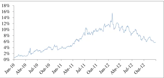
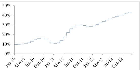
Figure 1: Yield spread between the 10 year Portuguese government bond and the German bond of the same maturity.
2
Descriptive statistics of all variables are presented in table 6 in Appendix 2. Graphs for all explanatory variables are presented in figures 4a-j also in Appendix 2.
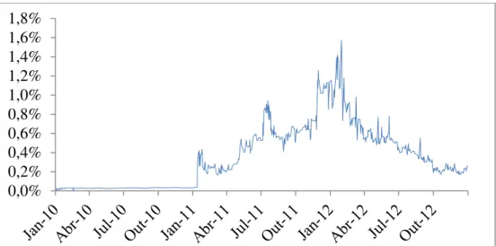
11 The proxy used to assess the international risk aversion factor is the spread
between the yield on 10 year, AAA rated US corporate bonds and the 10 year US
government bond yield. Daily data collected from Datastream.
To measure the credit risk of the Portuguese government three variables are
used: the debt to GDP ratio, the government balance in % of GDP and the growth rate
of real GDP. Quarterly data of the debt to GDP ratio is taken from Eurostat and then
interpolated to higher frequency (monthly). Because the estimation is conducted using
daily data observations for this variable and all other non-daily variables are updated
whenever a new observation exists. Quarterly data of the government’s revenues and
expenses and GDP is collected from Eurostat. The government balance in % of GDP is
then easily calculated. Finally, quarterly data on the annual level of real GDP is taken
from the OECD website and then interpolated to higher frequency (monthly). The
growth rate of real GDP is then easily calculated.
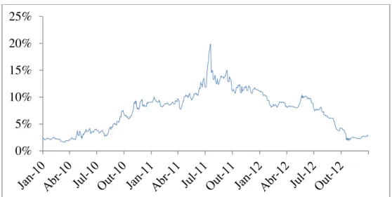
Bid-ask spreads are used as a proxy to gauge liquidity risk. Daily data is
collected from Bloomberg.
The variable used to assess the impact of the financial system on the government
yield spread is total banking assets in % of GDP. Monthly data of the aggregate banking
assets is available on Datastream.
All three fundamental, the liquidity risk and the financial system variables are
measured in differences to the corresponding German factor.
To measure contagion risk the probability of default3 is extracted from the 5 year
CDS spreads of four EMU governments (Greece, Ireland, Italy and Spain)4. Daily data
is available on Datastream. This variable is not measured in differences compared to the
3
Probability of default = CDS Spread/(1-Recovery Rate); Recovery rate assumed to be 40%. 4
12 German value which means that there is an implicit assumption that contagion effects
stemming from these countries did not affect the German government bond yield. This
does not seem that far-fetched since the German government was never considered to be
in any kind of financial trouble during the crisis, even when the aforementioned
countries were facing difficulties. Therefore, the contagion from the four countries
mentioned above will impact the dependent variable solely through the Portuguese yield
and the coefficient associated with each country are expected to be positive (the higher
the probability of default of each of the other EMU countries the greater the risk their
problems will spillover to Portugal and consequently the higher the Portuguese yield
spread.
Finally, weekly dummy variables on important events5 are also utilized to
measure their specific impact on the Portuguese yield spread: (12/3/10) approval of the
2010 budget, the last with sustainable bond yields; (20/4/10) publication of an IMF
report that puts Portugal as the second biggest source of financial distress in the EMU;
(25/5/10) budget cuts undertaken in Italy and Spain; (23/3/11) Portuguese government
resignation; (29/3/11) Portuguese government debt downgraded to one level above
“junk” status by Moody’s and Fitch; (6/4/11) Portugal asks for international help;
(4/8/11) the ECB buys Portuguese and Irish government debt.
IV. THE MODEL
Due to the high persistence of the dependent variable a dynamic model
specification is adopted to control for the past values of the yield spread. Taking into
account the difference in explanatory variables the estimated model is similar to that
estimated by Giordano, Linciano, Soccorso (2012):
5
13
(1)
∑
∑
Spread refers to the spread between 10 year Portuguese government bonds and
the German bond of similar maturity. Risk_aversion corresponds to the difference
between the yields of US 10 year, AAA graded corporate bonds and the 10 year US
government bond while debt, balance and growth represent the fundamental variables
proxied by debt to GDP ratio, government balance in % of GDP and growth rate of real
GDP, respectively (all measured in differences to the German values). Liquidity denotes
the difference between the Portuguese and German bid-ask spreads and bank_assets
designate the difference between the Portuguese and German banking assets in % of
GDP. Contagion designates a set of variables measuring the contagion risk stemming
from Greece, Ireland, Italy and Spain. Finally, dummy refers to the set of weekly
dummy variables used to assess the impact of specific events during the sample period.
The estimation is conducted using the OLS methodology with heteroskedasticity
and autocorrelation robust standard errors. Firstly, daily data ranging from January of
2010 to December of 2011 is used in the estimation. This sample period captures the
massive increase in the yield spread as can be observed in Figure 1.
Before proceeding with the estimation, however, the possible nonstationarity of
the variables must be taken into account to avoid a spurious regression. All variables are
integrated of order 16 at the 5% significance level and cointegrated7 at the 1%
significance level. This means there is an equilibrium relationship between the variables
which eliminates the spurious regression problem.
6
14 The cointegrating regression is presented below, in equation 2:
(2)
∑
The error correction model presented in equation 3, below, is estimated to gauge
the short run dynamics of the variables and assess which are the biggest contributors for
the variation of the yield spread in the short-run.
(3)
∑
The d(...) refers to the first-difference of a series and resid refers to the residuals
of the cointegrating regression 2.
Finally, regression 1 is re-estimated (without the dummy variables) for the
period ranging from March of 2012 until December of 2012 to determine if the drop of
the yield spread was driven (or not) by the same factors that previously led it to rise.
V.1 ESTIMATION RESULTS (Jan 10 – Dec 11)
In table 1 below, the results of the model specified in equation 1 are presented:
Table 1: Dynamic model (sample: January 2010 – December 2011)
Variables Coefficients Dummy variables Coefficients
intercept -0.00354 *** 2010_budget_approval 0.00087 *** spreadt-1 0.78514 *** IMF_report 0.00177 ***
risk_aversion 0.05155 budget_cuts_Spain_Italy -0.00085 ** debt 0.02840 *** government_resignation 0.00093 ** balance -0.00681 ** rating_cuts 0.00144 ***
growth -0.04729 Portugal_help 0.00088 **
liquidity 0.41419 ** ECB_buys_debt -0.00167 *** bank_assets 0.00588 ***
contagion_Greece 0.00392 ***
contagion_Ireland 0.04506 *** N 520
contagion_Italy 0.00454 Sample 4/1/10 – 30/12/11 contagion_Spain 0.05685 * R squared 0.996
15 The first lag of the dependent variable is extremely significant which is an
indication of the high persistence of the series.
The international risk aversion factor is not significant meaning that the causes
of the increase in the yield spread between 2010 and 2012 were not the same as those
back in 2008-2009: according to Attinasi, Checherita, Nickel (2009) the risk factor was
by far the main determinant of the rise in yield spreads during the 2008 financial crisis.
This result, however, makes sense because the level of global risk aversion is higher
during the 2008 financial crisis than afterwards during the Euro sovereign debt crisis
(this can be observed in figure 4a in Appendix 2).
Of the three fundamental variables used to assess the state of the Portuguese
government, two help to explain the rise in the yield spread: the debt to GDP ratio and
the government balance in % of GDP. The investors’ thus seem to place much more
importance in these two variables than in the growth rate of the economy. This is not
surprising since the reduction of the government budget deficit was top priority first for
the Portuguese government and also afterwards for the troika. Also the vast increase of
the debt to GDP ratio has naturally worried investors’ regarding Portugal’s long term
ability to honor these commitments so it is no surprise that they placed great importance
on this indicator. Finally, achieving GDP growth was never a priority of the Portuguese
authorities during this period which means that the recessions experienced by Portugal
were to be expected and did not overly concern investors.
Liquidity risk is also significant at the 5% significance level and positively
correlated with the yield spread meaning that an increase in the bid-ask spread of the 10
16 The variable controlling for the size of the banking system is also highly
significant and positively affects the yield spread, as would be expected. This may
suggest that investors were in fact worried about the possibility that the Portuguese
government would be forced to compromise its fiscal position in order to ensure the
stability of the financial system.
Contagion risk is also highly significant: contagion effects stemming from
Greece and Ireland are significant at the 1% significance level and those stemming from
Spain are significant at the 10% significance level. Only Italy’s coefficient is not significant. These results indicate that Portugal’s yield spread was negatively affected
primarily by the countries that requested international aid and by its neighboring
country whose much speculated collapse would have generated very serious systemic
problems for the EMU.
Finally, the dummies on specific events:
- 12nd of March 2010: the Portuguese Parliament approves the government budget
proposal for the year that would decide if Portugal needed international help or if it
could resolve its financial problems on its own. The markets reactions to the
approval of the budget were not positive because in the subsequent week the yield
spread of Portuguese government debt rose.
- 20th of April 2010: IMF report that puts Portugal as the second biggest source of
financial distress in the EMU. As it can be easily deduced this to widen the
Portuguese yield spread.
- 25th of May 2010: this dummy variable is useful for two reasons: it allows not only
to capture the 24 thousand million euros budget cuts in Italy (approved by the
17 Spain approved just 2 days later. This contributed to reduce the Portuguese yield
spread through the reduction in contagion risk. The significant at the 10% level
contagion effect obtained for Spain versus the insignificant Italian contagion effect
indicates that it is likely that most of the influence of this variable comes from the
Spanish austerity package.
- 23rd of March 2011: Portuguese prime-minister resigns creating a political crisis.
Naturally, this political uncertainty and need for anticipated elections contributed to
the expansion of the Portuguese yield spread.
- 29th of March 2011: this variable also captures two important events in the same
week: rating agencies, Moody’s (at the 29th) and Fitch (at the 1st of April) both
downgrade the Portuguese rating in the same week to one level above “junk” status.
This obviously led to an increase of the Portuguese yield spread.
- 6th of April 2011: Portugal asks for international help. This event also contributed to
amplify the Portuguese yield spread. Investors may have interpreted this as an
admission of the failure of the government measures and as a sign that the
government’s finances were actually in worse shape than had been described.
- 4th of August 2011: the ECB buys Portuguese and Irish government debt. The ECB
stepped in to help distressed countries which was interpreted as an sign that the ECB
would from then on adopt a more proactive stance in helping the countries in need.
This obviously contributed for the lowering of the Portuguese government bond
yield compared to Germany. This highlights the need for a wider, pan-European
response to the crisis.
18 Having already determined which factors played a role in the increase of the
Portuguese government bond yield in comparison to Germany it is now useful to
determine the relative contribution of each factor individually. In order to calculate this,
the methodology used in Attinasi, Checherita, Nickel (2009) is applied. As an example,
the relative contribution of the debt to GDP ratio to the increase in the Portuguese yield
spread is calculated in the following way:
(4)
| |
| | | | | | | | | | | | | | | | ∑ | | | |
The results are presented in the following graph:
Figure 2: Individual relative contributions of each factor. 8
As is apparent in the graph the greatest contributor for the increase in the yield
spread was the deterioration of the debt to GDP ratio in comparison to Germany. This
further supports the idea that investors are seriously worried with the accumulation of
8
The lagged dependent variable is not included in this calculation because the objective is to discern among the other explanatory variables which were the most important and not analyze the persistence of the series.
36%
2% 8%
6% 8% 25%
14%
0% 10% 20% 30% 40% 50% 60% 70% 80% 90% 100%
19 debt by the Portuguese government. The government balance had a small magnitude in
explaining changes in the yield spread.
Liquidity risk explained 8% of the evolution of the yield spread while banking
assets account for 6% of the change in the yield spread during this period. This indicates
that while investors were concerned about the financial capability of the Portuguese
government to ensure the stability of the banking system, they never believed that the
Portuguese banks would be sources of major problems.
Finally, the contagion effects: Ireland seems to be the biggest source of
contagion to Portugal followed by Spain and Greece. While Spain is a peripheral
country like Portugal and rumors were rampant at some point about a possible
intervention in the country the fact is that Spain never requested international help
which means that it makes sense that an intervened country (Ireland) is the one that
most contributes to Portugal’s contagion risk. The lower contagion risk stemming from
Greece points to the fact that investors though the context of Greek and Portuguese
situation was different. This makes sense since Portugal did not need a second rescue
package, social upheaval in Portugal is much less significant than in Greece,
fundamental data was not as bad to begin with and as bad as the political situation can
be in Portugal it still is more stable than in Greece.
Figure 2 further demonstrates that, on an aggregate level, fundamentals and
contagion risk were clearly the two main drivers of the increase of the Portuguese
government bond yield spread. Some policy implications can be drawn from this:
- The austerity route seems to be justified: if the main goal of the intervention of the
IMF/European Commission is to allow the Portuguese government to return to the
20 variables is the way to do it even if it compromises the growth rate of the economy -
a variable investors did not seem to take into account.
- European wide action is key to resolve this problem: while these conclusions
provide some support for the austerity route followed by the troika, contagion
effects were still the main drivers of the increase of the yield spreads. This means
that when one member country of the EMU faces problems the entire union must
swiftly react to provide financial and political support in order to keep the problems
from spreading. As this crisis demonstrated there are still a lot of deficiencies in the
way the EMU is organized especially in the political front with national elections
often getting in the way of what is in the best interest of the EMU.
- The implementation of Basel III, a tougher regulation for the banking system, is a
step in the right direction if the objective is to limit the spreading of private sector
risk to the public sector.
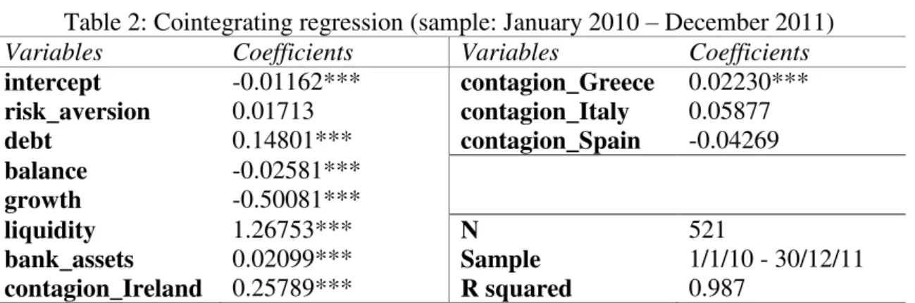
V.2 ESTIMATION RESULTS (Cointegrating Regression and EC Model)
In table 2 below, the results of the model specified in equation 2 are presented:
Table 2: Cointegrating regression (sample: January 2010 – December 2011)
Variables Coefficients Variables Coefficients
intercept -0.01162*** contagion_Greece 0.02230*** risk_aversion 0.01713 contagion_Italy 0.05877 debt 0.14801*** contagion_Spain -0.04269 balance -0.02581***
growth -0.50081***
liquidity 1.26753*** N 521
bank_assets 0.02099*** Sample 1/1/10 - 30/12/11 contagion_Ireland 0.25789*** R squared 0.987
Note: ***, **, * denote significance at 1, 5 and 10% levels, respectively.
Table 2 presents the long run determinants of the Portuguese government bond
yield spread. Results are very similar to those obtained in the dynamic model with only
21 stemming from Spain becomes non-significant. Despite the few changes they could
have strong implications on the conclusions taken in the previous section: if the growth
rate of real GDP is a significant determinant of the Portuguese yield spread the austerity
strategy may not be as appropriate as it seemed with the dynamic model.
Relative contribution of factors
Figure 4, however, shows that the previous section’s conclusions are still
accurate because despite turning significant, the relative contribution of the growth rate
of real GDP for the change of the yield spread is residual.
Figure 3: Individual relative contributions of each factor (cointegrating regression).
The main difference between this and figure 2, besides the different variables
used, is the increased importance of the debt to GDP ratio and of the contagion effect
stemming from Ireland. It also shows that in the long run the aggregate magnitude of
fundamental variables is greater than that of contagion effects (47% vs 43% in the long
run compared to 38% vs 47% in the dynamic model).
After assessing the long run effects of each variable, the ECM model specified
in equation 3 is estimated below to determine their short run effects. 42%
2% 3% 6% 5%
32% 11%
0% 10% 20% 30% 40% 50% 60% 70% 80% 90% 100%
22 Table 3: Error Correction Model (sample: January 2010 – December 2011)
Variables Coefficients Variables Coefficients
intercept 0.00020** d(contagion_Ire t-1) 0.08242**
d(spread t-1) 0.01673 d(contagion_Ita t-1) -0.06697
d(risk_aversion t-1) 0.14060 d(contagion_Spa t-1) 0.18441*
d(debt t-1) -0.00234 cointegration_eq_res t-1 -0.12249***
d(balance t-1) -0.00236
d(growth t-1) -0.16810
d(liquidity t-1) 0.02232 N 519
d(bank_assets t-1) 0.00429 Sample 5/1/10 - 30/12/11
d(contagion_Gre t-1) -0.00402 R squared 0.091 Note: ***, **, * denote significance at 1, 5 and 10% levels, respectively.
Error correction models are useful in order to determine the speed of
convergence of the dependent variable after a shock. This model also allows us to
understand the short term effects of the explanatory variables on the dependent variable.
The estimated coefficient of the error correction term is negative and significant which
means that deviations from the equilibrium value of the yield spread are corrected at
12% per day. Also the only significant explanatory variables are the Irish and Spanish
contagion effects (at the 5 and 10% levels, respectively). This means that these are the
two variables that significantly impact yield spreads in the short-run.
V.3 ESTIMATION RESULTS (Mar 12 – Dec 12)
At this point it makes sense to analyze if the drop of the Portuguese government
bond yield spread is explained by the same factors that led to its increase. The
estimation results are presented below, in table 3.
Firstly, it should be noted that two months were dropped from the estimation
period one before and one after the highest value of the yield spread (30th of January
2012). The estimation results were too sensitive to these outliers so they were dropped
23 Table 4: Dynamic model (sample: March 2012 – December 2012) 9
Variables Coefficients Variables Coefficients
c 0.02329* contagion_Ireland -0.07246
Spreadt-1 0.92572*** contagion_Italy 0.16692
risk_aversion -0.27227 contagion_Spain -0.07773
debt -0.03526
balance -0.01353
growth 0.40198 N 217
liquidity 0.45892 Sample 2/2/12 - 31/12/12
bank_assets -0.01089 R squared 0.985
Note: ***, **, * denote significance at 1, 5 and 10% levels, respectively.
No previously significant variable is significant anymore. Table 4 proves that the
great reduction of the 10 year Portuguese government bond yield spread in relation to
Germany was not due to an improvement in any of the variables that drove yields sky
high back in 2010-2011. This suggests that something other than these explanatory
factors is driving the yield spread10. Perhaps, the fact that Portugal is currently under the
tutelage of international institutions has lent credibility to its policies and thus assured
investors that Portugal is on the right track. If this is the case, though, a serious problem
will arise in 2014 when said international institutions are scheduled to leave the country.
VI. CONCLUSION
The Portuguese yield spread in relation to Germany sky rocketed in the period
between 2010 and 2011. This paper finds that the main drivers of this sharp increase
were fundamental variables (debt ratio and government balance), liquidity risk, the risk
of a government intervention in the financial system in order to ensure its stability and
contagion risk (stemming from Greece, Ireland and Spain). Fundamental variables and
contagion risk are the variables that boast the highest relative contributions.
9
There is no sovereign CDS data for Greece past end-February 2012 meaning that for this estimation the variable measuring the effect of contagion stemming from Greece is lost. This is not ideal but the estimated model below is still valid.
10
24 Two interesting policy implications can be derived from this:
- If the goal is to get the Portuguese government to return to the market as soon as
possible the austerity receipt was correct: fundamentals had a huge importance
during the crisis and thus must be greatly improved for Portugal to have any hope to
return to the markets.
- The EMU must be swifter in dealing with problems to one of its member countries:
contagion effects were the main drivers of the increase in yield spreads and the only
they can be minimized is if the EMU works quickly and as a unit to prevent these
contagion effects. There are, however, still many national political barriers getting in
the way for what is best for the EMU as a whole.
Finally, between March 2012 and the end of the year the yield spread dropped
significantly. Nonetheless, this drop was not supported by the same explanatory factors
that led it to increase dramatically in the previous two years. Non measurable factors
may be the leading cause for this decrease of the yield spread, namely the heightened
confidence that investors put in the international institutions that are currently
overseeing the Portuguese government. If this is the case it is likely that when these
institutions leave the country in 2014 the yield spread will increase again.
REFERENCES
- Aßmann, C. and Boysen-Hogrefe, J. (2009). Determinants of government bond
spreads in the euro area in good times as in bad. Kiel Working Paper 1548.
- Attinasi, M., Checherita, C. and Nickel, C. (2009). What explains the surge in Euro
area sovereign spreads during the financial crisis of 2007-09?, ECB WP No. 1131.
- Bernoth, K. and Erdogan, B. (2010). Sovereign Bond Yield Spreads: A Time-Varying
25 - Bernoth, K., von Hagen, J. and Schuknecht, L. (2004). Sovereign risk premia in the
European government bond market, ECB Working Paper (WP) No. 369.
- Caceres, C., Guzzo, V. and Segoviano, M. (2010). Sovereign Spreads: Global Risk
Aversion, Contagion or Fundamentals?, IMF WP/10/120.
- Codogno, L., Favero, C. and Missale, A. (2003). Yield spreads on EMU government
bonds, Economic Policy, October, pp. 505–532.
- De Grauwe, P. and Ji, Y. (2012). Mispricing of Sovereign Risk and Multiple
Equilibria in the Eurozone, CEPS Working Document No. 361.
- Flemming, M. J. (2003). Measuring treasury market liquidity. Economic Policy
Review, 9: 83-108.
- Gerlach, S., Schulz, A. and Wolff, G. B. (2010). Banking and sovereign risk in the
euro area, Discussion paper series 1: Economic studies, Deutsche Bundesbank.
- Giordano, L., Linciano, N. and Soccorso, P. (2012). The Determinants of Government
Yield Spreads in the Euro Area, CONSOB Working Papers No. 71.
- Klepsch, C. (2011). Yield Spreads on EMU Government Bonds - During the Financial
and the Euro Crisis.
- MacKinnon, J. G. (2010). Critical Values for Cointegration Tests, Working Papers
1227, Queen's University.
- Schuknecht, L., von Hagen, J. and Wolswijk, G. (2010). “Government Bond Risk
APPENDIX 1
Table 5: Sample periods of the papers referenced
Paper Sample period
Aßmann, C. and Boysen-Hogrefe, J.
(2009) From January 2001 until March 2009
Attinasi, M., Checherita, C. and Nickel, C. (2009)
From 31 July 2007 until 25 March 2009
Bernoth, K. and Erdogan, B. (2010) From Q1-1999 until Q1-2010
Bernoth, K., von Hagen, J. and
Schuknecht, L. (2004) From 1991 until 2002
Caceres, C., Guzzo, V. and
Segoviano, M. (2010) From mid-2005 until early-2010
Codogno, L., Favero, C. and Missale,
A. (2003) From 1999 until 2002
De Grauwe, P. and Ji, Y. (2012) From Q1-2000 until Q2-2011
Gerlach, S., Schulz, A. and Wolff, G. B. (2010)
From January 1999 until February 2009
Giordano, L., Linciano, N. and
Soccorso, P. (2012) From January 2002 until May 2012
Klepsch, C. (2011) From January 2000 until September 2010
Schuknecht, L., von Hagen, J. and
APPENDIX 2
Table 6: Descriptive statistics
Sample: 1/1/10 – 31/12/11
Mean St. dev. Max Min
Spread 5.1% 3.2% 12.0% 0.6%
Risk aversion 0.8% 0.1% 1.2% 0.4%
Debt 17.9% 7.5% 29.9% 9.7%
Balance -4.6% 5.0% 3.2% -10.1%
Growth -0.3% 0.3% 0.3% -0.8%
Liquidity 0.3% 0.3% 1.3% 0.0%
Banking assets 13.8% 10.1% 28.5% -5.0%
Contagion_Greece 30.3% 35.4% 184.9% 3.8%
Contagion_Ireland 7.8% 4.1% 19.9% 1.6%
Contagion_Italy 3.2% 1.9% 8.3% 1.2%
Contagion_Spain 3.5% 1.2% 6.7% 1.2%
Sample: 1/3/12 – 31/12/12
Mean St. dev. Max Min
Spread 8.6% 1.8% 12.3% 5.6%
Risk aversion 0.9% 0.2% 1.3% 0.6%
Debt 37.9% 3.5% 43.1% 32.0%
Balance -6.4% 2.8% -2.4% -9.5%
Growth -0.4% 0.1% -0.2% -0.5%
Liquidity 0.4% 0.2% 1.0% 0.2%
Banking assets 24.2% 5.0% 35.8% 18.4%
Contagion_Greece No data
Contagion_Ireland 6.2% 2.8% 10.4% 1.9%
Contagion_Italy 5.3% 1.4% 7.9% 3.0%
Contagion_Spain 5.5% 1.4% 8.2% 3.2%
Figure 4a: Difference between US 10 year, AAA graded corporate bonds and the 10year US government bond. 0,0% 0,5% 1,0% 1,5% 2,0% Ja n-07 Abr -07 Jul-07 Out-0 7 Ja n-08 Abr -08 Jul-08 Out-0 8 Ja n-09 A br -09 Jul-09 Out-0 9 Ja n-10 Abr -10 Jul-10 Out-1 0 Ja n-11 Abr -11 Jul-11 Out-1 1 Ja n-12 Abr -12
Jul-12 O
Figure 4b: Difference between the Portuguese and German debt to GDP ratios.
Figure 4c: Difference between the Portuguese and German government balances in % ofGDP.
Figure 4d: Difference between the Portuguese and German growth rates of real GDP.
Figure 4e: Difference between the Portuguese and German bid-ask spreads.
Figure 4f: Difference between the Portuguese and German banking assets in % of GDP.
Figure 4g: Greek government’s probability of default.
0,0% 0,2% 0,4% 0,6% 0,8% 1,0% 1,2% 1,4% 1,6% 1,8%
-10% -5% 0% 5% 10% 15% 20% 25% 30% 35% 40%
Figure 4h: Irish government’s probability of default.
Figure 4i: Italian government’s probability of default.
Figure 4j: Spanish government’s probability of default.
0% 5% 10% 15% 20% 25%
0% 1% 2% 3% 4% 5% 6% 7% 8% 9%
APPENDIX 3
Table 7: P-values of the unit root tests conducted on each variable (Null hypothesis: series has a unit root).
Sample: 1/1/10 – 31/12/11 Sample: 1/3/12 – 31/12/12 Levels Differentiated Levels Differentiated
Spread 26% 0% 29% 0%
Risk aversion 11% 0% 19% 0%
Debt 98% 0% 0% 0%
Balance 12% 0% 44% 0%
Growth 42% 0% 91% 0%
Liquidity 52% 0% 0% 0%
Banking assets 23% 0% 76% 0%
Contagion_Greece 100% 0% No data No data
Contagion_Ireland 10% 0% 69% 0%
Contagion_Italy 83% 0% 50% 0%
Contagion_Spain 9.4% 0% 42% 0%
Table 8: Engle Granger two-step tests on the regressions in tables 1 and 3, respectively (Null hypothesis: residuals of the cointegrating regression have a unit root).
Sample: 1/1/10 – 31/12/11
β∞ -6.22103 1% critical value -6.30147
β1 -41.7154 Test result -7.36611
β2 -102.68 Null hypothesis is rejected at the 1%
significance level ⇒ Residuals do not have a unit root ⇒ Series are cointegrated.
β3 389.33
N 521
Sample: 1/3/12 – 31/12/12
β∞ -4.696 10% critical value -4.769
β1 -15.732 Test result -3.61302
β2 -6.922 Null hypothesis cannot be rejected at the
10% significance level ⇒ Residuals have a unit root ⇒ Series are not cointegrated.
β3 67.721
N 218