Mixture models in quantitative genetics and applications to animal breeding

ISSN impresso: 1516-3598 ISSN on-line: 1806-9290 www.sbz.org.br

R. Bras. Zootec., v.36, suplemento especial, p.171-183, 2007

Correspondências devem ser enviadas para: gianola@ansci.wisc.edu

Mixture models in quantitative genetics and applications

to animal breeding

Daniel Gianolaa,c*_{; Paul J. Boettcher}b_{; Jørgen Ødegård}c_{; Bjørg Heringstad}c

a - Department of Animal Sciences. University of Wisconsin-Madison. Madison, WI 53706, USA. b - Institute of Biology and Biotechnology of Agriculture National Research Council. Segrate 20090. Italy.

c - Department of Animal and Aquacultural Sciences. Norwegian University of Life Sciences. P.O. Box 5025, N-1432 Ås Norway. Running head: Mixture models in animal breeding

ABSTRACT - Finite mixture models are helpful for uncovering heterogeneity due to hidden structure; for example, unknown major genes. The first part of this article gives examples and reviews quantitative genetics issues of continuous characters having a finite mixture of Gaussian components. The partition of variance in a mixture, the covariance between relatives under the supposition of an additive genetic model and the offspring-parent regression are derived. Formulae for assessing the effect of mass selection operating on a mixture are given. Expressions for the genetic correlation between a mixture and a Gaussian trait are presented. If there is heterogeneity in a population at the genetic or environmental levels, then genetic parameters based on theory treating distributions as homogeneous can lead to misleading interpretations. Subsequently, methods for parameter estimation (e.g., maximum likelihood) are reviewed, and the Bayesian approach is illustrated via an application to somatic cell scores in dairy cattle.

Key Words: Bayesian methods, dairy cattle, maximum likelihood, mixture distributions, quantitative

genetics, somatic cell scores

Introduction

Linear models with mixed effects have been used extensively in animal breeding since the early 50´s (e.g., Henderson, 1973). An account of the theory can be found in Searle et al. (1992), whereas Bayesian treatments are in Gianola & Fernando (1986) and Sorensen & Gianola (2002). Mixed linear models are flexible and can be fitted in cross-sectional, longitudinal, spatial or multi-response settings. In animal breeding, these models are used to infer genetic parameters such as heritability and genetic correlations, linear combinations of fixed effects (e.g., diferences in mean value of cohorts born in successive generations), and to predict breeding values of candidates for selection. Animal breeding implementations typically involve large data sets and hundreds of thousands of correlated random effects due to coancestry relationships between animals (Gianola, 2001).

However, linear models do not accommodate well discrete and censored variates and may not

be robust enough when there is “concealed” structure in the data.

Finite mixture models, used in biology and in genetics since Pearson (1894), are helpful for uncovering heterogeneity due to hidden structure or incorrect assumptions. The objective of this article is to review some aspects related to analysis with finite mixture models in animal breeding contexts. The paper is organized as follows. First, examples are presented where mixture models can play a useful role, followed by some basic statistical and quantitative genetics issues. Subsequently, maximum likelihood estimation of parameters of a mixture is discussed. Since use of Bayesian methods is exploding in biology, a brief account of a Bayesian application of mixtures to dairy cattle data is presented. The paper ends with concluding remarks.

Examples

©

illustrate, consider four problems arising in animal genetics. Unknown loci with major effects can create “bumps” (sometimes quite subtle) in a phenotypic distribution, and this heterogeneity may be resolved by fitting a mixture, i.e., by calculating conditional probabilities that a datum is drawn from one of the several potential, yet unknown, genotypes. A brief review of the use of mixtures for uncovering major genes is in Lynch & Walsh (1998). Also, many quantitative trait loci (QTL) detection procedures are based on ideas from mixture models (Haley & Knott, 1992). Basically, given marker and phenotypic data, one computes the probability that an individual has genotype QQ; Qq or qq at a putative QTL.

The second example is from dairy cattle breeding. Mastitis is an infammation of the mammary gland of cows associated with bacterial infection. Genetic variation in susceptibility to the disease exists, and genetic selection for resistance is a feasible strategy (Heringstad et al., 2000). However, routine recording of mastitis events is not conducted in most nations. Instead, milk somatic cell scores (SCS) measured in cows have been used as a proxy for the disease in genetic evaluation of artificial insemination bulls (with Gaussian mixed effects models), much as the prostate specific antigen is treated as a proxy for prostatic cancer. It is not obvious how SCS information should be treated optimally in genetic evaluation, because normal, clinical and different types of subclinical cases are hidden. Some of the challenges may be met using finite mixture models, as suggested by Detilleux & Leroy (2000), Ødegård et al. (2003, 2005), Gianola et al. (2004) and Boettcher et al. (2005, 2007).

Another example is from transcriptional analysis and genomics. In microarray studies, messenger RNA samples are collected from 2 target tissues, converted into complementary DNA, labelled with dyes of different colors (typically red and green), and hybridized against thousands of known pieces of DNA (genes) spotted in a slide. If a gene is expressed in the targets, hybridization is detected via fluorescence. Some spots are green, others red, plus every color in between! Image analysis is used for quantitating the extent of hybridization and differential expression. Observed expression may not reflect true differential expression, however. One can think in terms of a

mixture of at least 2 distributions:

1) if there is differential expression, the distributions of measurements in the red and green channels for a given gene would have different parameters, and

2) in the absence of differential expression, these parameters should be equal.

The fourth example is that of assessing genetic change in populations of animals subject to artificial selection. Animals are born, die or are culled at any point in time, so generations overlap. Since many such animals have unknown parents, it is difficult to give a crisp definition of “generation”. Animal breeders “group” individuals into more or less arbitrary cohorts (Quaas, 1988; Westell et al., 1988). However, the “true” group structure might be finer or coarser. An alternative to arbitrary grouping is to assume that unobservable genetic effects of unknown parents are drawn from a mixture of distributions.

Statistical and quantitative genetic ISSUES 100

Density, mean and variance. A random variate y (the distinction between variables and realized values is ignored in the notation) is drawn from one of K mutually exclusive and exhaustive distributions (groups), without knowing which of these underlies the draw. For instance, the observed SCS in the milk of a cow may be from a healthy or from an infected animal; if the disease is mastitis, the case may be clinical or subclinical. In the absence of a precise veterinary diagnosis, there is uncertainty about to which group the observed SCS score pertains to. Here, K = 3 and the underlying groups are: uninfected, clinical and sub-clinical. The density of y can be written as

where

K (assumed known) is the number of components of the mixture; Piis the probability that the draw is from the ith_{component; pi (y|θθθθθ}

i) is

©

respectively, where is the residual or environmental variance. Informally,

is the part of the

environmental variance contributed by population heterogeneity.

Assume that the genetic effect aiis also drawn from the mixture with GA components

(6) subject to . In general, y may be either scalar

or vector valued, or may be discrete. Here, we consider the situation where component distributions are Gaussian. In what follows, the notation N (y|µ,σ2_{) will denote a univariate normal}

distribution or density with mean µ and variance

σ2; whereas N (_y|_µµµµµ,_Σ) pertains to a multivariate

normal setting, where µµµµµis the mean vector and Σ is the variance covariance matrix.

The mean and variance of a finite mixture of K Gaussian distributions, with now θθθθθ = [P1, P2, ..., PK, µ1, µ2..., µK, , , ... , ]´, are

(1) and

(2)

The first term in (2) can be construed as the

average variance, whereas

measures dispersion between group means; if the µ´s are equal, this second term is null. Note that the variance of the mixture depends not only on the group variances, but on the group means as well.

The additive genetic mixture model

The quantitative genetics of characters distributed as mixtures has not been studied extensively, although the idea underlies work of, e.g., Latter (1965) and Kimura & Crow (1978). What follows is a summary of results in Gianola et al. (2006). Suppose an observable random variable (yi; phenotype of individual i) is drawn from

the finite mixture of GE Gaussian components

, (3)

and

(5)

where is a vector containing the mixing proportions (summing to 1); µe and are each

GE x 1 vectors of means and variances with typical elements µk and , respectively; ai is the genetic value of i. The mean and variance of this conditional (given the genetic effect) distribution are

(4)

k= 1

e e

where

pa = [Pa1, ..., PaG_A]´; αα ααα= [α1,...αGA]´, and

= [ , ... ]´ are the vectors of mixing

proportions, component means and component variances, respectively.

Then, and

(7)

where is the genetic variance, and

is interpretable as variance between genetic means. In Gaussian linear models the distribution of the random genetic effects is often taken to be N ; where is the additive genetic variance, so it may be

reasonable to introduce the restriction

in the mixture (Verbeke & Lesaffre, 1996). The joint density of ai and yi is obtained by multiplication of (3) and (6), yielding

(8)

©

kmth component; note that From standard Gaussian linear models theory, given the km component (let the indicator δkm = 1 denote such situation)

where N2 (.|.,.) denotes a bivariate normal distribution. Further

where

and

Under the standard additive genetic model, this regression of “genotype on phenotype”bkm is the heritability of the character under the kmth component of the bivariate mixture. The joint density (8) is also expressible as

(9)

The marginal density of yi is arrived at by integrating (9) over ai; yielding

(10)

This is a finite mixture of GE x GA univariate normal distributions with mixing proportions

. The mean and variance of the phenotypic distribution are

(11) and

(12)

A standard problem in quantitative genetics is that of inferring genetic values from phenotypes. From (9) and (10), the density of the conditional distribution of ai given yi is

(13)

where

Hence, the conditional distribution of ai given yi is a mixture of the GE x GA normal distributions, where the mixing proportion is Qkm, the conditional probability that the datum is drawn from ; given the observation yi. The best predictor of genetic value is the conditional expectation function (Henderson 1973; Bulmer 1980; Fernando & Gianola 1986).

(14)

©

(15)

In the standard additive genetic linear model, the variance of the conditional distribution of genotypes given phenotypes is , where h2 is the coefficient of heritability; this conditional variance is homogeneous and does not depend on the data. In a mixture model, however, the dispersion about the regression function is heteroscedastic and non-linear on the phenotypic value. Hence, both point and interval prediction of genetic value in mixtures involve strikingly different formulae.

Truncation selection

Consider the standard truncation selection setting in which individuals kept as parents are such that yi > t; with the proportion of individuals selected being Pr (yi > t) = γ. From (10), the distribution of phenotypic values within selected individuals has density

,

(17) where ikm is the selection intensity factor under the kmth component and

are relative weights summing to 1. The phenotypic superiority of selected individuals, or selection differential (S) is given by the difference between (17) and (11). Further, the mean genetic value of selected parents is

where

(16)

Above, γkm is the proportion selected within the kmth _{mixture component and Φ(.) is the}

standard normal distribution function. The proportion selected γ is, thus, a weighted average of the individual component selection proportions

γkm. Since the threshold is fixed, the components that are most prevalent, have largest means and are most variable, will be influential.

The mean value of selected individuals is

This expression cannot be evaluated analytically, because it is a highly nonlinear function of the phenotypic values. Finally, the genetic superiority of accepted parents over the unselected population is

The expected fraction of the selection differential that is realized can be assessed as

∆a/S; and this will differ from what could be

expected from the regression of offspring on mid parent, because of non-linearity.

Heritability

The fraction of variance attributable to additive genetic effects (usual definition of heritability) is location invariant for a Gaussian trait, i.e., it does not involve mean values. In a mixture, heritability becomes

(18)

©

component-specific variances ( and ), on mixing proportions ( and ) and on mean values (µk and αm) as well. In the simpler case in which the genetic distribution is the homogeneous process N (ai|0, ); “heritability” becomes

(19)

situations with different additive genetic variance ( ) and distances between means (∆) in the two distributions of the mixture: 1) = 1, ∆ = 1; 2) = 1, ∆ = 2; 3) = .10, ∆ = 1, and 4) = .10, ∆ = 2. Situations (1) and (2) correspond to a trait with a heritability of .50 under homogeneity, while (3) and (4) are for a lowly heritable trait (h2

≈

.09). In (1) and (2), the regressionβ decreases from 0.25 to about 0.22 and 0.17; respectively, representing relative decreases in heritability of 12 and 32%. The relative decreases in heritability are 18 and 47% in cases (3) and (4), respectively. In brief, heritability in heterogeneous or admixed populations depends on the mixing proportion, on the mean difference between mixture components and on the “homogeneous situation” heritability.

Correlations with a Gaussian trait

Correlations between a mixture trait and a normally distributed character (ω) may be of interest. For example, the mixture trait could be SCC in dairy cattle, with several component distributions corresponding to different unknown statuses of mammary gland disease. The Gaussian trait could be milk yield of a cow. Is the genetic correlation between the two traits affected by heterogeneity of somatic cell count?

The effect of on the genetic correlation is illustrated next for a 2-component mixture. Let be a heteroscedasticity factor, where , the genetic variance under the first component of the mixture, is viewed as “baseline” genetic variance, i.e., a measure of variability in the absence of heterogeneity. Then, it can be shown that under some simplifying assumptions and this is expected to be lower than in a

homogeneous population because fixed effects contribute to variance.

Offspring-parent regression.

The standard formula for the regression of the phenotypic value of a progeny (O) on that of a parent (P) gives

If the distribution of genetic effects is homogeneous, this simplifies to

(20)

The consequences are clear: if there is heterogeneity either in the distribution of sampling model residuals or of genetic effects, then βOP is affected by the mixing proportions and by the means µk. To illustrate, suppose that the genetic distribution is homogeneous; let GE = 2, take µ1 = 0 as origin,µ₂ = and Then (20) is expressible as

When Pe = 1; the formula gives half of heritability, which is a standard result. The function is symmetric with respect to Pe; since Pe (1 - Pe) is maximum at ; the regression is minimum at this value. As an example, consider the offspring-parent regression as a function of Pe for four

where is the genetic correlation in the

absence of a mixture and is

©

for two values of (0.7 and 0.3) and of λ

(1.5 and 2). As increases, the proportion of the component with the smaller genetic variance (m = 1) to increase.The genetic correlation increases monotonically with , the less variable component, and more rapidly so at the largest value of genetic heteroscedasticity. Similar algebra and considerations hold for the environmental correlation between traits.

Figure 1 - Genetic correlation (Rho) between a Gaussian character and a mixture trait for a two-component mixture, as a function of the mixing proportion ( ), for different combinations of = genetic correlation in absence of mixture and λ= heteroscedasticity factor. From top to bottom: 1) = 0.7, λ= 1.5 (open squares); 2) = 0.7, λ = 2 (dotted line); 3) = 0.3, λ = 1.5 (solid line); 4) = 0.3, λ= 2 (open circles).

Summary remarks

If there is heterogeneity in a population either at the genetic or environmental levels, then genetic parameters based on theory treating distributions as homogeneous can lead to misleading interpretations. Some peculiarities of mixture characters are: heritability depends on the mean values of the populations, the offspring-parent regression is non-linear, and genetic or phenotypic correlations cannot be interpreted devoid of the mixture proportions and of the parameters of the component distributions.

Maximum likelihood estimation

Motivation

Detilleux & Leroy (2000) pointed out advantages of a mixture model for analysis of SCS in dairy cows. The mixture model can account for effects of infection status on SCS and produce an estimate of prevalence of infection, plus a

probability of status (infected versus un-infected) for individual cows, given the data and values of the parameters. Detilleux & Leroy (2000) proposed a 2-component mixture model, which will be referred to as DL hereafter. Although additional components may be required for finer statistical modelling of SCS, our focus will be on a 2-component specification, as a reasonable point of departure. An important issue is that of parameter identification. In likelihood inference this can be resolved by introducing restrictions in parameter values, although creating computational difficulties. In Bayesian settings, proper priors solve the identification problem. A Bayesian analysis with Markov chain Monte Carlo procedures is straightforward, but priors must be proper. However, many geneticists are refractory to using Bayesian models with informative priors, so having alternative methods of analysis available is desirable. Hereafter, a normal mixture model with correlated random effects is presented from a likelihood-based perspective.

Hierarchical DL

The mixture model is developed hierarchically. Let P be the probability that a SCS is from an uninfected cow. Unconditionally to group membership, but given the breeding value of the cow, the density of observation i (i = 1, 2, ..., n) is Mixing proportion Pal

Rho

where yi and ai are the SCS and additive genetic value, respectively, of the cow on which the record is taken, and β= [β´0; β´1]´. The probability that the draw is made from distribution 0 is supposed constant from individual to individual.

Assuming that records are conditionally independent, the density of all n observations, given the breeding values, is

(21)

©

(22) and the marginal density of the data is

(23)

When viewed as a function of the parameters

´

(23) is Fisher´s likelihood. This can be written as the product of n integrals only when individuals are genetically unrelated; here, would not be identiable. On the other hand, if ai represents some cluster effect (e.g., a

sire’s transmitting ability), the between-cluster variance can be identified.

DL assume normality throughout and take and Here, x’0i and x’1i are known incidence vectors relating fixed effects to observations. The assumption about the genetic effects is a|A, ~ N (0,A ). Let now zi~ Bernoulli (P), be an independent (a priori) random variable taking the value zi = 0 with probability P if the datum is drawn from process N0; or the value zi = 1 with probability 1 - P if from N1. Assuming all parameters are known, one has

(24)

Thus,

is the probability that the cow belongs to the infected group, given the observed SCS, her breeding value and the parameters.

A linear model for an observation (given zi) can be written as

A vectorial representation is

where Diag(z_i) is a diagonal matrix with typical

element zi; X0 is an n x p0 matrix with typical row x’0i; X1 is an n x

p1 matrix with typical row x’1i; a = {ai} and e = {ei}. Specific forms of β₀ and β₁ (and of the corresponding incidence matrices) are context-dependent, but care must be exercised to ensure parameter identifiability and to avoid what is known as label switching. For example, DL take X0β0= 1µ0 and X1β1= 1µ1.

EM Algorithm

One can extremize (23) with respect to

θ

θθ

θ

via the expectation-maximization algorithm, or EM. An EM version with stochastic steps was developed by Gianola et al. (2004). The EM algorithm augments (22) with n binary indicator variables zi (i = 1, 2, ..., n), taken as independently and identically distributed as Bernoulli; with probability P. If zi= 0; the SCS datum is generated from the uninfected component; if zi= 1; the draw is from the other component. Let z = [z1, z2, ..., zn]´ denote the realized values of all z variables. The complete data is the vector [a´, y´, z´]´, with [a´, z´]´ constituting the

missing part and y representing the observed fraction. The joint density of a, y and z can be written as

(25)

Given z; the

component of the mixture generating the data is known automatically for each observation. Now

for i = 1,2,...,n. Then, (25) becomes

(26)

©

Genetic evaluation for SCS could be based on

i

â , the ith element of â, the mean vector of the distribution

While 2

e 1 0,β,σ

β and P follow from the maximum

likelihood procedure, â must be calculated more conveniently using Monte Carlo methods. Another issue is how the SCS information is translated into chances of a cow belonging to the uninfected group. A simple option is to estimate (24) as

(27)

assess which model was most appropriate for use in genetic evaluation of SCS. A brief account of this study is given here.

Data

Test-day records from primiparous Holstein cattle in 105 large (>200 cows) herds primarily in Wisconsin) were used. The somatic cell count records had been converted to linear somatic cell scores (SCS), using a standard log 2 transformation. Because herds were well-managed, the mean SCS of around 2.20 was less than the US national average of approximately 3.00. The dataset analyzed included 177,846 records from 31,040 cows, daughters of 3,082 different sires. An additive relationships file was created by tracing pedigrees at least 3 generations, including ancestors that were related to at least 2 animals with records. The pedigree file included 54,143 animals.

^ ^ _^ ^

^ ^ ^ ^

^ ^ ^ ^ ^ ^

^

^ ^ ^ ^ _{^ ^ ^}

Statistically (27) does not take into account the error of the maximum likelihood estimates of all parameters. If the likelihood function is sharp and unimodal (large samples), this is a minor concern.

Bayesian analysis with case study

Ødegård et al. (2003) developed a Bayesian approach for analysis of a 2-component mixture model for SCS with heterogeneous residual variances, and applied it to simulated data. Their model considered heterogeneity of variances for residual effects only, and it was extended subsequently, to derive a criterion suitable for selection against putative mastitis by Ødegård et al. (2005). If SCS is a trait that differs genetically between infected and uninfected cattle, allowing for heterogeneity of genetic and permanent environmental (PE) variances may be appropriate. Boettcher et al. (2007) allowed for heterogeneous variances of genetic and PE effects, and, applied the mixture models to data on SCS collected in US Holsteins. Several models of increasing levels of complexity were compared for fit, in an attempt to

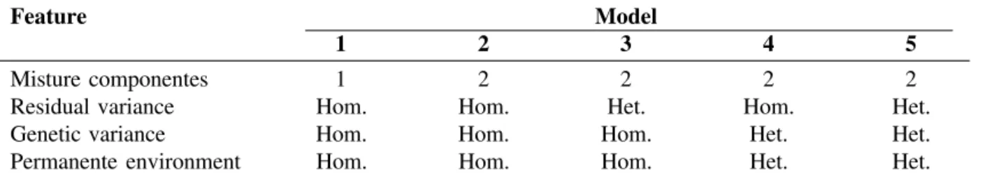
Table 1 - Summary of the 5 models tested1_.

Feature Model

1 2 3 4 5

Misture componentes 1 2 2 2 2

Residual variance Hom. Hom. Het. Hom. Het.

Genetic variance Hom. Hom. Hom. Het. Het.

Permanente environment Hom. Hom. Hom. Het. Het.

1 - Hom = Homogeneous variance; Het = Heterogeneous variance.

Figure 2 - Source: Boettcher et al. (2007).

Models

Five different models were fitted (Figure 2). Model 1 was a standard test-day repeatability model. Fixed effects of systematic non-genetic factors and random additive genetic and PE effects were fitted. The other 4 specifications were 2-component Gaussian mixture models differing according to the type of heterogeneity of variances considered. All 3 variances (additive, PE, and residual) were homogeneous for Model 2, whereas all variances were heterogeneous for Model 5. Analyses were based on previous work of Ødegård et al. (2003), with some extensions to accommodate Models 4 and 5.

For the mixture models, observations of SCS were assigned to 1 of the 2 components, assumed to be indicative of health status. Assignments were defined by a (unknown) vector z, where zi= 0 for a

©

record i from a healthy cow and zi = 1 for records from infected cows. Following the notation used by Ødegård et al. (2003), the equations for the various models can be written, given z, as shown in Figure 3. The fixed effects in β0 included 3

regression coeficients for effects of days in milk on SCS, 17 effects of age at calving, and 3,361 herd-test-day effects. Regression coefficients for days in milk were based on the curve by Wilmink (1987). Age-at-calving effects were one for each age from 20 through 36 months. The β1 vector included a

single element, the mean difference (shift) between components 1 and 2. For the non-mixture model (Model 1), all elements of Mz were zero. For models with homogeneous genetic and PE variances (i.e., Models 1, 2, and 3), a0 = a1 and p0= p1. For these

models, a0 ~N(0, A ), where A is the numerator

relationship matrix and is the additive genetic variance, and p0 ~ N(0, Iσ2p), where I is an identity

matrix of order 31,040 and 2 p

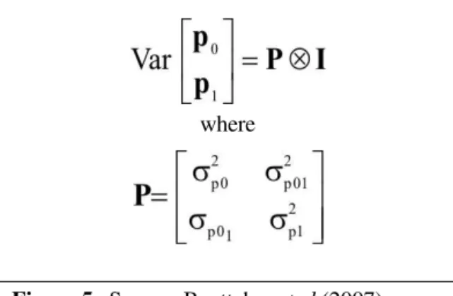
σ is the permanent environmental variance. When genetic and PE effects were heterogeneous, expectations of a0, a1, p0 and p1 where all zero. The covariance sctructure

of genetic and PE effects was as in Figures 4 and 5, respectively. There, G is the variance-covariance matrix between additive genetic values under the healthy and diseased statuses Further, P is the variance-covariance matrix between corresponding PE effects. Conditionally on the breeding values and PE effects, the variance matrix of the observation vector (residual variance matrix) was expressed as in Figure 6, where I is an identity matrix of order n and and are residual variances for observations from the first and second components, respectively. For models with homogenous residual variance, (i.e., Models 1, 2, and 4) Equation (4) simplifies to R = I .

Bayesian Analysis

Briefly, a Gibbs sampler was run in which all unknown parameters and the indicator z were drawn from their conditional posterior distributions. Five sampling chains of 205,000 cycles each were generated for each model. For each chain, the first 5,000 cycles were discarded as burn-in period so that a total of 1,000,000 posterior samples were available for each model. Convergence was assessed by the approach of Gelman et al. (2004). Posterior distributions of (co)variances were assessed based

on sampling every 20th cycle. Posterior means for breeding values were obtained by averaging realizations from every 500th cycle.

y = X0βββββ0 + MzX1βββββ1 + (I-Mz)Zaa0

+ MzZaa1 + (I-Mz)Zpp0 +MzZpp1 +e,

Figure 3 - Source: Boettcher et al. (2007).

where y = vector of n observations for test-day SCS, β0 = vector of fixed effects commom to all

records; β1 = vector of fixed effects

corresponding to observation from infected cows; I = identity matrix of order n; M_z = matrix with diagonal elements corresponding to vector z; a0 = vector of randon additive genetic effects

on SCS in the healthy state; a1 = vector of

random additive genetic effects on SCS in the infected state; p0 = vector of random PE effectos

in the healthy state; p1= vector of random PE

effects in the infection state; e = vecor of residual effects; and X0, X1, Za and Zp = incidence

matrixes corresponding to fixed (X.) and random (Z.) effects, respectively.

Figure 4 - Source: Boettcher et al. (2007).

where

Figure 5 - Source: Boettcher et al.(2007).

R = (I - Mz)σ2e0+ Mzσ2e1

© Comparison of models

The models were compared based on the Deviance information criterion (DIC) proposed by Spiegelhalter et al. (2002). The model with the lowest DIC is considered to be the most appropriate model statistically.

Estimated breeding values (EBV) resulting from the different models were evaluated for similarity. The posterior means of additive genetic effects (calculated by sampling every 500th cycle) were used as EBV. Pearson correlation coefficients were calculated between all pairs of the 7 sets of animal solutions: 1 set of EBV from each of the 3 models (1, 2, and 3) with homogeneous genetic variance and 2 sets each from the 2 models (4 and 5) with heterogeneous genetic variance. Correlation coefficients were calculated for 2 sets of animals: 1) all animals, N = 54,143, and 2) only sires with at least 10 offspring (N = 541). To examine changes in rank, all sires with at least 10 offspring were sorted in ascending order based on each of the 7 sets of EBV. Then, the top and bottom 50 sires were identified for each set. Finally, the number of animals in common between each pair (high ranking with high ranking and low vs. low) of these sets was observed. Low numbers of mismatches were assumed to indicate high similarity among evaluation models.

for the diseased component of the mixture. No obvious trend was observed for genetic variance when comparing the standard model with the 4 mixture models. In Model 4, the estimates of genetic and PE variances for the second component were much larger than the variances obtained by either of the other 3 mixture models. The genetic variance of the second component was 2.41 in Model 4, versus 0.52 for Model 5; corresponding PE variances were 3.22 and 0.76, respectively.

According to the DIC, Model 4 was favored, by far; recall that a model with the lowest DIC is preferred. The DIC of Model 1 was twice as large as for any of the mixture models. The correlations among EBV from the different pairs of models were all about 0.90. Despite high correlations among EBV, the degree of sire re-ranking among models indicated that the use of a mixture model would lead to real changes in sire selection if applied instead of the linear model. For all mixture models (Models 2 through 5), the top 50 sires (low SCS) differed by at least 10 sires (>20%) from the top 50 identified by the linear model (Model 1). Eleven sires were in common among the top 50, and 13 were in common among the bottom 50.

Conclusion

Based strictly on statistical considerations, mixture models are more appropriate for analysis of, e.g., SCS data of dairy cattle than standard linear models. In the case studied, a shuffling in order of the highest ranked sires was observed, demonstrating that practical differences would be realized with the adoption of a mixture model for genetic evaluation.

Although the statistical evidence supporting the use of mixture models is strong, questions remain about the biological ramifications of applying a mixture model, and about the precise meaning of the different EBV resulting from a mixture model with heterogeneous genetic effects. Another issue is how a genetic evaluation for SCS can be translated into a selection criterion, as discussed in Ødegård et al. (2005).

A challenge for scientists confronted with massive data sets, such as those in animal breeding and in gene expression analysis, is making the computations needed for implementing the mixed effects mixture models (MMM) feasible. Gianola Results

©

et al. (2004) described a maximum likelihood analysis of a Gaussian mixture with random effects using the EM algorithm with a Monte-Carlo E-step. Ødegård et al. (2003) presented a Gibbs sampling scheme for a Bayesian hierarchical 2-component mixture model (with thousands of random effects), and retrieved accurate estimates of parameters in simulation studies. While Markov chain Monte Carlo may be the only way of carrying out a fully Bayesian analysis, diagnosing convergence to the equilibrium distribution is a serious problem for models with thousands of unobservable random effects. Similarly, non-Bayesian analysis may be carried out more efficiently with algorithms based on second derivatives than with EM; in the latter, augmenting the likelihood with indicator variables (so that the missing data fraction becomes very large) can slowdown convergence painfully.

Standard models for quantitative traits can lead to erroneous results if fitted to heterogeneous data. If a mixture is suspected, two of the most suitable methods for inferring unknown mixture parameters are maximum likelihood and Bayesian analysis. Procedures for likelihood or posterior-based inference applied to mixtures are discussed extensively in Titterington et al. (1985) and McLachlan and Peel (2000), including situations in which the component distributions are not-normal, e.g., skewed survival processes.

Implementations suitable for fitting different types of quantitative genetic mixture models have been described and applied by Ødegård et al. (2003, 2005), Gianola et al. (2004), and Boettcher et al. (2005, 2007). Prediction of breeding values is discussed in Gianola (2005). A convenient software for the analysis of mixtures with random effects is available in a forthcoming update of Version 6.0 of the DMU package described in Madsen & Jensen (2002).

Literature cited

BOETTCHER, P.J.; MORONI, P.J.; PISONI, G. et al.

Application of a finite mixture model to somatic cell scores of Italian goats. Journal of Dairy Science, v.88, p.2209-2216, 2005.

BOETTCHER, P.J.; CARAVIELLO, D.; GIANOLA, D. Genetic analysis of somatic cell Scores in US Holstein

with a Bayesian mixture model. Journal of Dairy

Science, v.90, p.435-443, 2007

BULMER, M.G. The Mathematical Theory of

Quantitative Genetics. Clarendon Press, Oxford. 1980.

DETILLEUX , J.; LEROY, P.L. Application of a mixed normal mixture model to the estimation of mastitis-related parameters. Journal of Dairy Science, v.83, p.2341-2349, 2000

FERNANDO, R.L.; GIANOLA, D. Optimal properties of the conditional mean as a selection criterion.

Theoretical and Applied Genetics, v.72, p.822-825. 1986.

GELMAN, A.; CARLIN, J.B.; STERN, H.S. et al. Bayesian data analysis, 2nd edn. Chapman and Hall, Boca Raton. 539, 2004

GIANOLA, D.; FERNANDO, R.L. Bayesian methods in animal breeding theory. Journal of Animal Science, v.63, p.217-244, 1986.

GIANOLA, D. Inferences about breeding values. In

Handbook of Statistical Genetics (D.J. Balding, M. Bishop and C. Cannings, eds.) 645-672. Wiley, Bu¢ ns Lane. 2001.

GIANOLA, D. Prediction of random effects in finite

mixture models with Gaussian components. Journal

of Animal Breeding and Genetics, v.122, n.546, p. 145-160, 2005.

GIANOLA, D.J., ØDEGÅRD, B., HERINGSTAD, G. et al.

Mixture model for inferring susceptibility to mastitis in dairy cattle: a procedurefor likelihood-based inference. Genetics, Selection, Evolution, v.36, p.3-27, 2004

GIANOLA, D.; HERINGSTAD, B.; ØDEGÅRD, J. On the quantitative genetics of mixture characters. Genetics, v.173, p.2247-2255, 2006.

HALEY, C.S.; KNOTT, S.A. A simple regression method for mapping quantitative trait loci in line crosses using .anking markers. Heredity, v.69, p.315.324, 1992

HENDERSON, C.R. Sire evaluation and genetic

trends. In Proceedings of the Animal Breeding and Genetics Symposium in Honor of Dr. Jay L. Lush 10-41. American Society of Animal Science and American Dairy Science Association, Champaign, IL. 1973 HERINGSTAD, B.; KLEMETSDAL, G.; RUANE, J.

Selection for mastitis resistance in dairy cattle: a review with focus on the situation in the Nordic countries.

Livest. Prod. Sci., v.64, p.95-106, 2000.

KIMURA, M.; CROW, J.F. Effect of overall phenotypic selection on genetic change at individual loci. Proc. Natl. Acad. Sci., v.75, n.567, p.6168-6171, 1978. LATTER, B.D.H. The response to arti.cial selection due

to autosomal genes of large effect. Aust. J. Biol. Sci., v.18, p.585-598, 1965.

LYNCH, M.; WALSH, B. Genetics and Analysis of Quantitative Traits. Sinauer, Sunderland. 1998. MADSEN, P. & JENSEN, J. A User.s Guide to DMU. A

package for analysing mixed models. Version 6, Release 4.3. 19pp. Danish Institute of Agricultural Sciences. 2002.

McLACHLAN, G. & PEEL, D. Finite Mixture Models. Wiley, New York. 2000.

ØDEGÅRD, J.; JENSEN, J.; MADSEN, P. et al. Mixture

models for detection of mastitis in dairy cattle using test-day somatic cell scores: a Bayesian approach via

Gibbs sampling. Journal of Dairy Science, v.86,

p.3694-3703, 2003.

ØDEGÅRD, J.; MADSEN, P.; GIANOLA, D. et al.

Threshold-Normal Mixture Model for Analysis of a Continuous Mastitis- Related Trait. J. Dairy Sci., v. 88, p.2652-2659, 2005.

PEARSON, K., Contributions to the mathematical theory of evolution. Phil. Trans. Roy. Soc. A v. 185, p.71-110 1894.

© 1338-1345, 1988.

SEARLE, S.R.; CASELLA, G.; McCULLOCH, C.E. Variance Components. Wiley, New York. 1992. SORENSEN, D.; GIANOLA, D. Likelihood, Bayesian and

MCMC Methods in Quantitative Genetics. Springer, New York. 2002.