Modelos de equações estruturais aplicados à genética quantitativa

“Luiz de Queiroz” College of Agriculture

Structural equation models applied to quantitative genetics

Pedro Henrique Ramos Cerqueira

Thesis presented to obtain the degree of Doctor in Science. Area: Statistics and Agricultural Experimentation

Structural equation models applied to quantitative genetics

versão revisada de acordo com a resoluçãp CoPGr 6018 de 2011

Advisor:

Prof. Dr. ROSELI APARECIDA LEANDRO

Co-Advisor:

Prof. Dr. GUILHERME JORDÃO DE MAGALHÃES ROSA

Thesis presented to obtain the degree of Doctor in Science. Area: Statistics and Agricultural Experimentation

Dados Internacionais de Catalogação na Publicação DIVISÃO DE BIBLIOTECA - DIBD/ESALQ/USP

Cerqueira, Pedro Henrique Ramos

Structural equation models applied to quantitative genetics / Pedro Henrique Ramos Cerqueira. versão revisada de acordo com a resolução CoPGr 6018 de 2011. -Piracicaba, 2015.

95 p. : il.

Tese (Doutorado) - - Escola Superior de Agricultura “Luiz de Queiroz”.

1. Inferência bayesiana 2. Modelos de equações estruturais 3. Genética quantitativa 4. Regressão polinomial 5. Modelos lineares mistos 6. Amostrador de Gibbs 7. Modelos mistos multi característicos 8. Gado leiteiro da raça Holandesa I. Título

CDD 636.214 C411s

DEDICATION

Firstly to God

Without him nothing would be possible

To my Mom,

Juraci Ramos Cerqueira (in memorian).

To my grandma,

Adelaide Ramos Cerqueira.

To my aunt,

Roseli Ramos Cerqueira.

To my lovely wife,

Camila Rodrigues Gonçalves Cerqueira.

To them,

I lovingly dedicate this work

ACKNOWLEDGMENTS

I would like to express my gratitude to all those who gave me the possibility to complete this thesis, especially to my grandma Adelaide Ramos Cerqueira, my aunt Roseli Ramos Cerqueira, my father Sérgio de Souza, for their love and supporting during all my life.

An especial thanks to my wife Camila Rodrigues Gonçalves Cerqueira, for supporting me during all academic formation, being my partner and helping me in my most important decision.

To my all family in-law, especially my father in-law Lourivalter (Seu Valter), mother in-law Maria Helena, sister in-law Isabella and grandparents in-law Joaquim and Yolanda, for all the support, and also, being so kind and lovely during those years.

To my advisor, Prof. Dr. Roseli Aparecida Leandro, for the continuous support of my all academic pathway, for her patience, motivation, enthusiasm and immense knowledge.

To my co-advisor Prof. Dr. Guilherme Jordão de Magalhães Rosa, for receiving me on my internship period and for being so helpful during my stay in Madison Wisconsin giving me all support that was needed.

To Bruno and Francisco Peñagaricano (Pancho), from University of Wisconsin, for their friendship, scientific contribution, intellectual input and especially for participating in the pro-cess of Doctorate.

To my especial friends from ESALQ, Mariana Ragassi Urbano, Rodrigo Rosseto Pescim, Luiz Ricardo Nakamura (Zan), Ana Julia Righetto, Thiago Gentil (Bem), Iuri Ferreira (Pipi) and Rafael Maia, who were always willing to help, also, for providing me a more enjoyable life in the last four years and for all discussion regarding ours carriers and “science” during the daily coffee breaks.

To my especial colleagues and friends from University of Wisconsin, Vivian Felipe, Tom Murphy, Llibertat, Ferran, Claudia, Rodrigo Pacheco, Renato Ribeiro and his family for all their support friendship helping me to have a more pleasure life during my stay in Madison.

To Prof. Dr. Taciana Villela Salvian, Prof. Dr. Cristian Marcelo Villegas Lobos and Prof. Dr. Clarice Garcia Borges Demétrio at ESALQ/USP and Prof. Dave L. Thomas at UW, for their valuable guidance and friendship. To Prof. Kent Weigel for conceding the data set for the analysis.

To my friends from the Department of Exact Science at ESALQ/USP, Cássio Dessotti, Gui-lherme Biz, Lucas Cunha, Edilan Quaresma, Ezequiel Lopez, Maurício Lordello, Djair (Dja-van), Everton da Rocha, Thiago Oliveira, Ricardo Klein, Maria Cristina Martins, Rafael Moral, Tiago Santana, Marcus Gurgel, Everton de Toledo Hanser and Altemir.

To the staff of the Department of Exact Science at ESALQ/USP, the secretaries Solange de Assis Paes Sabadin, Mayara Segatto, Rosni Pinto and Luciane Brajão, in special to the computer technicians Jorge Alexandre Wiendl and Eduardo Bonilha for always helping with techniques issues.

Luke: I don’t believe it,

Master Yoda: That is why you fail

SUMMARY

RESUMO . . . 11

ABSTRACT . . . 13

1 INTRODUCTION . . . 15

References . . . 17

2 GENERAL OVERVIEW . . . 23

Abstract . . . 23

2.1 Introduction . . . 23

2.2 Linear Mixed models . . . 24

2.2.1 General description . . . 25

2.2.2 Parameter estimation . . . 25

2.2.3 Restricted maximum likelihood . . . 26

2.2.4 Bayesian inference: an overview . . . 29

2.2.5 Linear mixed models in quantitative genetics . . . 32

2.3 Causal inference . . . 35

References . . . 37

3 ADVANTAGES OF USING HIGHER POLYNOMIAL INSTEAD OF LINEAR RELATIONSHIP BETWEEN TRAITS IN STRUCTURAL EQUATION MOD-ELS IN QUANTITATIVE GENETICS: A SIMULATION STUDY . . . 43

Abstract . . . 43

3.1 Introduction . . . 43

3.2 Material and Methods . . . 45

3.2.1 Methods . . . 45

3.2.2 Simulation data . . . 48

3.2.3 Analysis . . . 49

3.2.4 Results of fitting polynomial SEM . . . 50

3.2.5 Results of fitting SEM with linear effects . . . 57

3.2.6 Discussion . . . 62

3.3 Conclusion . . . 63

References . . . 64

4 USING POLYNOMIAL STRUCTURAL EQUATION MODELS TO ESTIMATE THE EFFECTS RELATED TO CALVING IN PRIMIPAROUS HOLSTEIN CATTLE . . . 67

Abstract . . . 67

4.1 Introduction . . . 67

4.2 Material and Methods . . . 69

4.2.1 Data . . . 69

4.2.3 Estimation and computation . . . 74

4.3 Results and Discussion . . . 75

4.3.1 Results of Multiple trait mixed models (fixed effects) . . . 75

4.3.2 Results of linear structural models (fixed effects) . . . 77

4.3.3 Results of second-degree polynomial structural models (fixed effects) . . . 79

4.3.4 Results of third-degree polynomial structural models (fixed effects) . . . 82

4.3.5 Results without causal relationships between GL and CD and second-degree poly-nomial structural models (fixed Effects) . . . 84

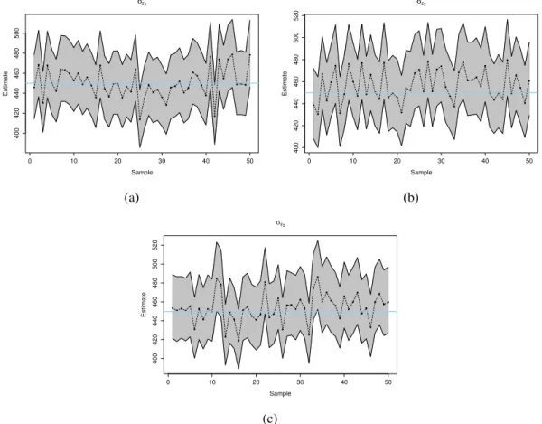
4.3.6 Results of variances-covariances components . . . 87

4.3.7 Discussion . . . 88

4.4 Conclusion . . . 89

References . . . 89

5 CONCLUSION . . . 95

RESUMO

Modelos de equações estruturais aplicados à genética quantitativa

Modelos causais têm sido muitos utilizados em estudos em diferentes áreas de conheci-mento, a fim de compreender as associações ou relações causais entre variáveis. Durante as últimas décadas, o uso desses modelos têm crescido muito, especialmente estudos relacionados à sistemas biológicos, uma vez que compreender as relações entre características são essenci-ais para prever quessenci-ais são as consequências de intervenções em tessenci-ais sistemas. Análise do grafo (AG) e os modelos de equações estruturais (MEE) são utilizados como ferramentas para explo-rar essas relações. Enquanto AG nos permite buscar por estruturas causais, que representam qualitativamente como as variáveis são causalmente conectadas, ajustando o MEE com uma es-trutura causal conhecida nos permite inferir a magnitude dos efeitos causais. Os MEE também podem ser vistos como modelos de regressão múltipla em que uma variável resposta pode ser vista como explanatória para uma outra característica. Estudos utilizando MEE em genética quantitativa visam estudar os efeitos genéticos diretos e indiretos associados aos indivíduos por meio de informações realcionadas aos indivíduas, além das característcas observadas, como por exemplo o parentesco entre eles. Neste contexto, é tipicamente adotada a suposição que as características observadas são relacionadas linearmente. No entanto, para alguns cenários, relações não lineares são observadas, o que torna as suposições mencionadas inadequadas. Para superar essa limitação, este trabalho propõe o uso de modelos de equações estruturais de efeitos polinomiais mistos, de segundo grau ou seperior, para modelar relações não lineares. Neste trabalho foram desenvolvidos dois estudos, um de simulação e uma aplicação a dados reais. O primeiro estudo envolveu a simulação de 50 conjuntos de dados, com uma estrutura causal com-pletamente recursiva, envolvendo 3 características, em que foram permitidas relações causais lineares e não lineares entre as mesmas. O segundo estudo envolveu a análise de características relacionadas ao gado leiteiro da raça Holandesa, foram utilizadas relações entre os seguintes fenótipos: dificuldade de parto, duração da gestação e a proporção de morte perionatal. Nós comparamos o modelo misto de múltiplas características com os modelos de equações estru-turais polinomiais, com diferentes graus polinomiais, a fim de verificar os benefícios do MEE polinomial de segundo grau ou superior. Para algumas situações a suposição inapropriada de linearidade resulta em previsões pobres das variâncias e covariâncias genéticas diretas, indire-tas e totais, seja por superestimar, subestimar, ou mesmo atribuir sinais opostos as covariâncias. Portanto, verificamos que a inclusão de um grau de polinômio aumenta o poder de expressão do MEE.

Palavras-chave: Inferência bayesiana; Modelos de equações estruturais; Genética quantitativa; Regressão polinomial; Modelos lineares mistos; Amostrador de Gibbs;

ABSTRACT

Structural equation models applied to quantitative genetics

Causal models have been used in different areas of knowledge in order to comprehend the causal associations between variables. Over the past decades, the amount of studies using these models have been growing a lot, especially those related to biological systems where studying and learning causal relationships among traits are essential for predicting the consequences of interventions in such system. Graph analysis (GA) and structural equation modeling (SEM) are tools used to explore such associations. While GA allows searching causal structures that express qualitatively how variables are causally connected, fitting SEM with a known causal structure allows to infer the magnitude of causal effects. Also SEM can be viewed as multiple regression models in which response variables can be explanatory variables for others. In quan-titative genetics studies, SEM aimed to study the direct and indirect genetic effects associated to individuals through information related to them, beyond the observed characteristics, such as the kinship relations. In those studies typically the assumptions of linear relationships among traits are made. However, in some scenarios, nonlinear relationships can be observed, which make unsuitable the mentioned assumptions. To overcome this limitation, this paper proposes to use a mixed effects polynomial structural equation model, second or superior degree, to model those nonlinear relationships. Two studies were developed, a simulation and an application to real data. The first study involved simulation of 50 data sets, with a fully recursive causal structure involving three characteristics in which linear and nonlinear causal relations between them were allowed. The second study involved the analysis of traits related to dairy cows of the Holstein breed. Phenotypic relationships between traits were calving difficulty, gestation length and also the proportion of perionatal death. We compare the model of multiple traits and polynomials structural equations models, under different polynomials degrees in order to assess the benefits of the SEM polynomial of second or higher degree. For some situations the inappropriate assumption of linearity results in poor predictions of the direct, indirect and total of the genetic variances and covariance, either overestimating, underestimating, or even assign opposite signs to covariances. Therefore, we conclude that the inclusion of a polynomial degree increases the SEM expressive power.

1 INTRODUCTION

Studies related to genetics are extremely important and they have been increasing during the past decades, in numbers and size of records, specially in areas such as medical sciences and agronomy. The computational advancement provides new techniques for acquisition and analysis of genetic data. In medical sciences, some techniques have been used for instance to detect genes associated to diseases, and in agriculture studies have been developed in order to improve the animal and plant breeding. Molecular technologies such as SAGE, microarray and RNA-seq, have been used to identify those genes associations, allowing the discovery of complex network of biochemical processes related to living organisms, common diseases in humans, gene discovery and structure determination (SCHADT et al., 2005; HUGHES et al., 2000; KARP et al., 2003).

In medical sciences, studies related to the most common problems such as heart diseases, osteoporosis, diabetes and cancer, have been developed using genetic and environmental in-formation. Such diseases are typically deemed as results of complex interactions of multiple genes and environmental aspects (LI et al., 2006; CHAIBUB NETO et al., 2008). Genetics associations between disease may be due to common genetic factors, or may occur due to phys-iological interactions. For instance, cardiovascular disease can be related to a plethora of traits, such as blood pressure, insulin levels, triglyceride and cholesterol levels (STOLL et al., 2001; NADEAU et al., 2003; SINICROPE; SARGENT, 2012).

In agronomy, specifically in animal breeding, there is an interest on studying the relation-ship between phenotypic traits such as growth, milk production and diseases. Generally, those studies involve others covariates, such as age, season and year, that can be common (the same) for all traits or specifics for some of them, also it is often incorporated information concerning to herds and especially family using some kinship information, for instance pedigree.

Most of genetics studies are based on traditional probabilistic models, where the response variables (i.e. traits of interest) are associated to covariates (ROSA et al., 2011). Those models are efficient in verifying how likely the occurrence of the characteristic of interest is. However, they are not efficient in predicting how the probability of a particular event can be affected by external interventions (ROSA et al., 2011; PEARL, 2009).

each other, however their relationship is given by a common effect, the rain. It is also possi-ble to find cases where one can not find a common factor among variapossi-bles, some examples of spurious correlations (e.g. Per capita consumption of mozzarella cheese with civil engineering doctorates awards) can be found onhttp://www.tylervigen.com/spurious-correlations.

All those connections among traits can be seen as a network, or phenotypic network, that explains which traits modify each other, or if a trait modify more than one trait, those modifi-cations can also be called as the effects caused by an specific trait. The effects can be positive or negative, but they do not necessarily present the same direction, for example: suppose two traitsy₁ andy₂, wherey₁ influencesy₂ positively, whiley₂ may have a positive, negative or

may not have any effect ony₁. Rosa et al. (2011) exemplifies this influence using the fact that

a high production in dairy cows can increase the chances of a certain type of disease, however, the occurrence of this disease can affect production negatively.

To study how traits are causally related and what is the magnitude of each pairwise relation-ship, causal inference models, or simply causal models, have been used (ROSA et al., 2011; FOX, 2008). The number of studies involving the inference of causal relationships has been in-creasing during the last two decades, specially in economy and social sciences, as for instance Fox (2008), Duncan et al. (1968), Ferron and Hess (2007) and Greene (2011). In genetics, those models have been used in order to discover, comprehend and explain gene networks for example Chaibub Neto (2010), Chaibub Neto et al. (2010), Rosa and Valente (2014), Gianola and Sorensen (2004), Shadt et al. (2005), Xiong et al. (2004) and others.

Two different approaches are used to investigate how variables are causally connected and to infer the magnitude of their causal relationships: the graph analysis (GA) and the tural equation models (SEM). The GA methods allow performing a search for causal struc-tures and help visualize those relations, i.e, they express qualitatively how the variables are causally connected (LIU et al., 2008;. LI et al., 2006, CERQUEIRA, et al., 2014). Some proce-dures to recover the causal relationships can be found in literature, e.g inductive causation (IC) and Peter-Clarck (PC) algorithms (GLYMOUR et al.,1986; PEARL, 2009; HARRIS; DRTON, 2013; ROSA et al., 2011; VALENTE et al., 2010).

as a procedure to estimate the coefficient based on latent structural models. Also packages such

assemandlavaanwere developed for the open software R (FOX, 2008; FOX, 2006).

In animal breeding studies, several traits are typically measured and modelled. Generally, these studies are performed using observational data, and also information related to environ-mental factors, e.g farms and cities, and genetic distance, e.g pedigree, are used for predicting individual genetic effects and estimating genetic parameters. The most common approach for those situations is the linear mixed model, where fixed and random effects are modeled at the same time (LAIRD; WARE, 1982; PINHEIRO; BATES, 2000; MRODE, 2005).

The amount of studies using SEM in quantitative have increased after Gianola and Sorensen (2004), they were the forerunners proposing mixed effects structural equation models, under which the authors adapted structural equation models to the mixed models context (VALENTE et al., 2011; VALENTE et al., 2013).

Studies involving SEM in quantitative genetics generally are developed under the assump-tion of linear causal relaassump-tionships among traits, which is not realistic in some situaassump-tions (MATU-RANA et al., 2009; GONZÁLES-RODRIGUÉZ et al., 2014; VARONA et al., 2014; KÖNIG et al., 2008). In order to show the underlying inference mistakes of using this commonly adopted assumption, this work propose an approach using structural equation model with higher order polynomials.

Chapter 2 introduces a general overview of important aspects to the issue here tackled. Chapter 3 shows a simulation study to compare the structural equation models using standard linear and the second degree polynomial approaches. In Chapter 4, an application related to calving traits in Holstein cows is used to illustrate how estimates change under different as-sumptions of polynomials degrees. Chapter 5 present a general conclusion and prospective works.

References

CERQUEIRA, P.H.R.; VALENTE, B.; ROSA, G.J.M; LEANDRO, R.A. Second degree polynomial structural equation modeling using animal model: A simulation study In:

INTERNATIONAL BIOMETRIC CONFERENCE, 27., 2014, Florence,Abstracts...

Florence: IBS, 2014.

CHAIBUB NETO, E..Causal inference methods in statistical genetics. Madison: University of Wisconsin, 2010. 140 p.

CHAIBUB NETO, E.; KELLER, M.P; ATTIE, A.D.; YANDELL, B.S.. Causal graphical models in systems genetics: A unified framework for joint inference of causal network and genetic architecture for correlated phenotypes. Annals Applied Statistic, Cleveland, v. 4, p. 320-339, 2010.

DUNCAN, O.D.; HALLER, A.O.; PORTES, A.. Peer influences on aspirations: A reinterpretation. American Journal of Sociology, Chicago, v. 74, p. 119-137, 1968.

FERRON, J.M.; HESS, M.R. Estimation in SEM: A concrete example. Journal of Educational and Behavioral Statistics, Washington, v. 32, p. 110-120, 2007.

FOX, J.. An introduction to structural equation modeling, curso para programa de Computação Científica, FIOCRUZ: Rio de Janeiro, Brasil , 2008. p. 138.

FOX, J.. Structural equation modeling with the sem package in R.Structural equation modeling, Hillsdale, v. 13, p. 465-486, 2006.

GIANOLA, D.; SORENSEN, D.. Quantitative genetic models for describing simultaneous and recursive relationships between phenotypes. Genetics, Baltimore, v. 167, p. 1407-1424, 2004.

GLYMOUR, C; SCHEINES, R.; SPIRTES, P.; KELLY, K.. Discovering Causal Structure: Artificial Intelligence, Philosophy of Science, and Statistical Modeling. Pittisburgh, Academic Press, 1986. 412 p.

GONZÁLEZ-RODRÍGUEZ, A.; MOURESAN, E.F.; ALTARRIBA, J.; MORENI, C.;

VARONA, L.. Non-linear recursive models for growth traits in the Pirenaica beef cattle breed. Animal : an international journal of animal bioscience, Cambridge, v. 8, p. 904-911, 2014.

GREENE, W.H.. Econometric analysis, 7 ed. New York, Macmillan. 2011. 1232 p.

HUGHES, T.R.; MARTON, M.J.; JONES, A.R.;, ROBERTS, C.J.; STOUGHTON, R.; A, C.D.; BENNETT, H.A.; COFFEY, E.; DAI, H.; HE, Y.D.; KIDD, M.J.; KING, A.M.; MEYER, M.R.; SLADE, D.; LUM, P.Y.; STEPANIANTS, S.B.; SHOEMAKER, D.D.;

GACHOTTE, D.; CHAKRABURTTY, K.; SIMON, J.; BARD, M.; FRIEND, S.H.. Functional discovery via a compendium of expression profiles.Cell, Cambridge, v. 2, p. 109-146, 2000.

JÖRESKPG, K.G.; SÖRBOM, D. LISREL III Computer software, Chicago, IL: Scientific Software International, Inc. 1974.

KARP, C.L.; GRUPE, A.; SCHADT, E.;EWART, S.L.;KEANE-MOORE, M.; CUOMO, P.J.; KÃHL, J.; Larry WAHL, L.;KUPERMAN, D.;GERMER, S.; AUD, D.;PELTZ, G.;

WILLS-KARP, M.. Identification of complement factor 5 as a susceptibility locus experimental allergic asthma.Nature Immunology, New York, v. 1, p. 221-226, 2003.

KÖNIG, S.; WU, X. L.; GIANOLA, D.; HERINGSTAD, B.; SIMIANER, H.. Exploration of relationships between claw disorders and milk yield in Holstein cows via recursive linear and threshold models.Journal of Dairy Science, Champaign, v. 91, p. 395-406, 2008.

LAIRD, N.M.; WARE, J.H. Random-Effects Models for longitudinal Data.Biometrics, Alexandria, v. 38, n. 4, p. 963-974, 1982.

LI, R.; TSAIH, SHING-WERN; STYLIANOU, I. M.; WERGEDAL, J.; PAIGEN, B.;

CHURCHILL, G.A.. Structural model analysis of multiple quantitative traits.PLoS Genetics, San Francisco, v. 2, p. 1046-1057, 2006.

LIU, B.; FUENTE, A. de la; HOESCHELE, I.. Gene network inference via structural equation modeling in genetical genomics experiments.Genetics, Baltimore, v. 178, p. 1763-1776, 2008.

MRODE, R. A..Linear Models for the Prediction of Animal Breeding Values, 2 ed. Wallingford, Oxon, UK: CAB International, 2005. 344 p.

PEARL, J.Causality Models, Reasoning and inference. 2 ed. Cambridge, RU: Cambridge University Press, 2009. 484 p.

PINHEIRO, J. C.; BATES, D. M..Mixed-Effects Models in S and S-PLAS. New York: Springer, 2000. 528 p.

R. Development Core Team. R Foundation for Statistical Computing. R 2.15.2: A language and environment for statistical computing, Vienna, 2012. Avaiable:

<http://www.r-project.org/>. Acess em: 23 nov. 2012

ROSA, G.J.M.; VALENTE, B.D. Structural Equation Models for Studying Causal Phenotype Networks in Quantitative Genetics in SINOQUETE, C.; MOURAD, R.. Probabilistic

Graphical Models for Genetics, Genomics and Postgenomics, Oxford University Press, Oxford, 2014. 480 p.

ROSA, G.J.M.; VALENTE, B.D.; de lo CAMPOS, G.; WU, X.L.; GIANOLA, D.; SILVA, M.A.. Inferring causal phenotype networks using structural equation models.Genetics, Selection, Evolution, London, v. 2, p. 1046-1057, 2011.

SCHADT, E.E.; LAMB, J.; YANG, X.; ZHU, J.; EDWARDS, S.; GUHATHAKURTA, D.; SIEBTS, S.K.; MONKS, S.; REITMAN, M.; ZHANG, C.; LUM, P.Y.; LEONARDSON, A.; THIERINGER, R.; METZGER, J.M.; YANG, L.; CASTLE, J.; ZHU, H.; KASH, S.F.; DRAKE, T.A.; SACHS, A.; LUSIS, A.J. An integrative genomics approach to infer causal associations between gene expression and disease. Nature Genetics, New York, v. 37, p. 710-717, 2005.

SINICROPE, F.A.; SARGENT, D.J. Molecular Pathways: Microsatellite Instability in Colorectal Cancer: Prognostic, Predictive and Therapeutic Implications. Clinical Cancer Resarch, Denville, v. 18, p. 1506-1512, 2012.

STOLL, M.; COWLEY JUNIOR, .A.W.; TONELLATO, P.J.; GREENE A.S.;KALDUNSKI, M.L.; ROMAN, R.J.; DUMAS, P.; SCHORK, N.J.; WANG, Z.; JACOB, H.J.. A

Genomic-Systems biology map for cardiovascular function.Science, Washington, v. 294, p. 1723-1726, 2001.

The TETRAD Project Causal Models and Statistical Data. tetrad. Avaiable:

VALENTE, B.D.; ROSA, G.J.M.; CAMPOS, G. de los; GIANOLA, D.; SILVA, M.A.. Searching for recursive causal structures in multivariate quantitative genetics mixed models. Genetics, Baltimore, v. 185, p. 633-644, 2010.

VALENTE, B.D.; ROSA, G.J.M.; SILVA, M.A.; TEIXEIRA, R.B.; TORRES, R.A.. Searching for phenotypic causal networks involving complex traits: an application to European quails. Genetics, Selection, Evolution, London, v. 43, p. 37-48, 2011.

VALENTE, B.D.; ROSA, G.J.M.; GIANOLA, D.; WU, X-L; WEIGEL. K.. Is Structural Equation Modeling Advantageous for the Genetic Improvement of Multiple Traits?Genetics, Baltimore, v. 194, p. 561-572, 2013.

VARONA, L.; SORENSEN, D.. Joint Analysis of Binomial And Continuous Traits with a Recursive Model: A Case Study Using Mortality and Litter Size of Pigs. Genetics, Baltimore, v. 196, p. 643-651, 2014.

VIGEN, T.Spurious Correlations. Avaiable in <http://tylervigen.com/spurious-correlations>. Acess:2 jun. 2014 .

2 GENERAL OVERVIEW

Abstract

Multivariate linear mixed models have been widely used in quantitative genetics to estimate the fixed effects and covariance components, as well as to predict random effects. Some envi-ronmental and genetic effects are typically treated as random effects related to each trait while other factors are treated as having fixed effects. However, standard mixed effects models traits do not take into account that traits may be causally related to each other. Nonetheless, several studies have verified that traits are connected because of some causal relationship. Causal effect models have been used as a tool to account for such relationships. The application of causal modeling involves two fundamentals aspects: graph analysis, to infer how traits are causally related, and structural equation modeling, to infer the magnitude of those effects. Restricted maximum likelihood and Bayesian inference approaches are typically applied for inferences. In order to have a better comprehension of aspects that will be covered in Chapter 3 and Chap-ter 4, a general overview associated with those concepts is presented in this chapChap-ter.

Keywords: Causal Models; Graph Models; Structural Models; Restricted Maximum Likelihood Linear Mixed Models; Quantitative Genetics; Bayesian Inference

2.1 Introduction

Studies related to quantitative genetics involve predicting genetic effects (random effects) and estimating effects related to covariates representing environmental factors (typically as-sumed to be fixed effects). Generally, the joint inference of those effects involves using single-trait or multiple-single-trait linear mixed models (MRODE, 2005; HENDERSON, 1975; ROSA; VA-LENTE, 2014; VALENTE et al., 2013; VALENTE et al., 2015; VALENTE; ROSA, 2013 ).

Although they are not expressed in the mentioned standard models, phenotypic traits can have mutually causal effects. Suppose that interventions can be made to increase milk yield. High milk production may increase the liability to certain diseases, and conversely, the in-cidence of a disease may affect yield negatively ( ROSA et al., 2011). In order to describe causal relationships and to predict the behavior of complex systems (e.g., biological pathways underlying complex traits related to diseases, growth, and reproduction), as well as possible consequences of external interventions, knowledge of phenotype networks is crucial (ROSA, et al. 2011; ROSA; VALENTE, 2014).

rela-tionships among traits in multivariate systems. According to Rosa et al. (2011), Pearl (2009) and Shipley (2004), SEM can be used as a general model to estimate and verify the relationships between traits. Before fitting SEM, it is necessary to define qualitatively how traits are causally connected, whether by using prior knowledge or alternative data-driven search procedures. This information forms the “causal structure”, and it is generally represented by a directed graph.

This chapter reviews some concepts that are important to the development of this thesis. In Section 2.1, an overview related to linear mixed models is presented, and Section 2.1.1 contains a general description. Section 2.1.2 introduces estimations methods and Section 2.1.3 presents some applications of mixed models in quantitative genetics. Finally, Section 2.2 presents a review of causal models.

2.2 Linear Mixed models

Studies in quantitative genetics usually take into account information related to environ-mental factors, e.g., farms and cities, and genetic information, e.g., pedigree, for predicting individual genetic effects and estimating genetic parameters. The most common approach used in these situations is a linear mixed model, where fixed and random effects are modeled jointly (LAIRD; WARE, 1982; PINHEIRO; BATES, 2000; MRODE, 2005)

An advantage of using mixed models is that they provide a flexible and powerful tool for the analysis of data. Observations are grouped over some average effects with random deviations from it, such that some dependency among observations in the same group is accounted for, which can be common in many diverse areas, such as agriculture, biology, economics and genetics. Examples of clustered data are longitudinal or family member studies. The latter is common in genetic studies (PINHEIRO; BATES, 2000; ROSA; VALENTE, 2014).

2.2.1 General description

According to Laird (1982), Pinheiro and Bates (2000), Rosa and Valente (2014) a mixed linear model can be presented as

y = Xβ+Zb+ε, (2.1)

whereyis the response vector, with dimension (n×1),βis a vector of fixed parameters with

dimension (p×1),bis a vector of unknown random effects with dimension (q×1),X andZare

known incidence matrices with dimension (n×p) and (n×q) related toβandb, respectively,

andε is the vector of residual terms with dimension (n×1). Usually, it is assumed thatband ε are independent and normally distributed with mean zero and variance-covariance matrices

equal toGandR, respectively.

One of the main goals of linear mixed model applications in animal and plant breeding is to predict random effects, especially the genetic merit, or breeding values. The predictions are given by the conditional expectation ofbgiven the data,E(b|y). The joint distribution ofyand bis a multivariate normal such as

y b ∼N Xβ 0 , V ZG

GZ′ G

(2.2)

whereV =ZGZ′ +R, and following multivariate normal distributions properties,E(b|y)is

given by

E(b|y) = E(b) + Cov(b,y′)Var−₁

(y)(y−E(y)),

= Cov(b,y′)Var−1(y)(y−E(y)),

= GZ′V−1(y−Xβ). (2.3)

WhenR = σ2_{Iand Z = 0, the mixed model in equation 2.1, is reduced to avstandard linear}

model, where the residual terms are assumed independent and there are no other random effects.

2.2.2 Parameter estimation

Assuming thatGandRare known andbandεare normally distributed, the density of the

distribution ofyis given by

f(y;θ) = 1 (2π)n/2_|ZGZ′

+R|1/2 exp

1 2

(y−Xβ)′

(ZGZ′+R−1(y−Xβ)

, (2.4)

whereθis the vector of parameters (b,β,G) and the joint probability density function,f(y,b) =

f(y|b)f(b)is given by

f(y,b) = 1

(2π)n/2_|R|1/2 exp

1 2

(y−Xβ−Zb)′

R−1(y−Xβ−Zb)

× 1

(2π)q/2_|G|1/2 exp

1 2b

′

G−1b

The logarithm of equation 2.5 is given by

ℓ(y,b) = 1

22nlog(2π)− 1

2(log|R|+ log|G|)

− 1

2 y

′

R−1y−2y′R−1Xβ−2y′R−1Zb+ 2β′X′R−1Zb

+ β′X′R−1Xβ+b′Z′R−1Zb+b′G−1b) (2.6)

Deriving equation 2.6 inβandband equating to0yields

X′R−1X X′R−1Z Z′R−1X Z′R−1Z+G−1

ˆ β ˆ b =

X′R−1y Z′R−1y

. (2.7)

From equation 2.7 it possible to obtain the best linear unbiased predictor (BLUP) ofb, given

by

ˆ

b = Z′R−1Z+G−1−1

Z′R−1(y−Xβˆ), (2.8)

and it is also possible to obtain the best linear unbiased estimator (BLUE) ofβˆ, given by

ˆ

β = {X′[R−1−R−1Z(Z′R−1Z+G−1)−1Z′R)]X}−1

× X′[R−1−R−1Z(Z′R−1Z+G−1)−₁

Z′R−1)]y (2.9)

It is possible to verify by some algebraic manipulation that the estimates of equations 2.8 and 2.9 are the same as the estimates presented in equation 2.3.

2.2.3 Restricted maximum likelihood

The restricted maximum likelihood (REML) method, developed in 1971 by Patterson and Thompson under the assumptions of normal distribution, has been widely used to estimate variance components in mixed models, because it takes into account the degrees of freedom involved in estimating the fixed parameters, providing a less biased estimate than the maximum likelihood (ML) estimate (PATTERSON; THOMPSON, 1971; HARVILLE, 1977; GILMOUR; THOMPSON; CULLIS, 1995). The REML maximizes the joint likelihood function of all con-trasts ofy∗

=L′y, whereLis a full rank matrix withn-rank(X) columns, and its columns are

orthogonal to the column space ofX, i.eL′X = 0. Thus the REML is a method that maximize the part of the maximum likelihood function that is invariant to fixed effects. LetL= [L1L2],

where

L′₁X =Ip and L

′

2X =0,

and lety∗

j =L

′

jy, j = 1,2theny

∗

1 andy

∗

y∗₁ = L′₁y

= Ipβ+L

′

1Zb+L

′

1ε,

and

y∗

2 = L

′

2y

= L′₂Zb+L′₂ε,

consequently,

E(y∗) = E

y∗ 1 y∗ 2 = β 0 (2.10) and

Var(y∗) = Var

y∗ 1 y∗ 2 =

L′₁V L₁ L′₁V L₂ L′₂V L₁ L′₂V L₂

, (2.11) thus, y∗ 1 y∗ 2 ∼N β 0 ,

L′₁V L1 L

′

1V L2 L′₂V L₁ L′₂V L₂

(2.12)

The complete distribution L′y can be split into a conditional distribution y∗

1|y

∗

2 and a

marginal distribution ofY∗₂ to estimateβand the variance components, respectively.

Assuming thatk′ = (γ′

,φ′)is the vector of variance components related tobandε,

respec-tively, their likelihood logarithms are given by

ℓR = −

1 2

log det(L′₂V−1L₂) +y₂′∗(L′₂V−1L₂)−₁

y]

− 1

2log det(X

′

V−1X) + log detV +y′P y, (2.13)

where

P =V−1−V−1X(X′V−1X)−₁

X′V−1, (2.14)

and

y′P y = (y−Xβˆ)′

V−1(y−Xβˆ). (2.15)

The REML estimates forklwherek= (k1, k2, . . . , kL)can be obtained by solving forkthe

U(kl) =

∂lR

∂kl

=−1

2 tr P∂V ∂kl

−y′P∂V

∂kl

P y

, (2.16)

and the elements of the observed and expected information matrix are give by

− ∂

2_l

R

∂kl∂kk

= 1 2tr

P ∂ 2_V

∂kl∂kk

−1

2tr

P∂V ∂kl

P∂V ∂kk

+ y′P∂V ∂kl

P∂V ∂kk

P y− 1

2y

′

P ∂ 2_V

∂kl∂kk

P y, (2.17)

and, E − ∂ 2_l R

∂kl∂kk = 1 2tr P∂V ∂kl P∂V ∂kk . (2.18)

However, to solve U(kk) = 0, it is necessary to use an iterative algorithm. Thus, given an

initial starting valuek(0), a new valuek(1) is obtained using the Fisher score algorithm, given

by

k(1) =k(0)+I(k(0),k(0))−₁

U(k(0)) (2.19)

where U(k(0)) is the score vector presented in equation 2.16 andI(k(0),k(0)) represents the

expected information matrix ofkpresented in equation 2.18, evaluated ink(0)_.

When using big datasets or data with high dimension, the evaluation of the traces in equa-tions 2.17 and 2.18 can be unfeasible or computationally intensive. For those cases Gilmour, Thompson and Cullis (1995) propose the average information (AI) algorithm which has con-vergence properties like the Fisher score algorithm, although avoiding the high computational effort.

The AI algorithm essentially works with a modified form of the expected information ma-trix. Instead ofI(kl, kk)it is usedIA(kl, kk)where

IA(kl, kk) =

1 2y ′ P∂V ∂kl P∂V ∂kk

P y. (2.20)

2.2.4 Bayesian inference: an overview

Bayesian inference allows modeling and expressing the parameters uncertainty using prior information, via known probability distributions. The Bayesian approach combines two sources of information: One is the data evidence, which is expressed by the likelihood function, and the other is information from prior knowledge of the modelâs unknown quantities, represented by the prior distribution. Updating the prior knowledge after considering the data evidence from the likelihood function involves combining both types of information according to Bayes theorem, obtaining 2.21.

P(θ|y) = P(y|θ)P(θ)

P(y) (2.21)

where P(y|θ) represents the likelihood, P(θ) represents the prior distribution, and P(θ|y)

is the so-called posterior distribution. P(y)for the continuous and discrete cases can be con-structed as in 2.22 and 2.23, respectively.

P(y) =

Z

θP(y,θ)dθ=

Z

θP(θ|y)P(θ)dθ (2.22)

and

P(y) = X

θ

P(y,θ) = X

θ

P(θ|y)P(θ). (2.23)

The functionP(y)is independent ofθ, and therefore can be considered a constant for the

posterior distribution. For this reason, equation 2.21 can be expressed as

P(θ|y)∝P(y|θ)P(θ). (2.24)

According to Box and Tiao (1992), the symbol of proportionality, represented by∝, holds

because the information fromp(y)does not contribute to the parameterâs posterior distribution.

The prior distribution expresses the uncertainty regarding the parameters before observing the data. Such information can be obtained by asking a specialist (or a researcher), or from re-sults provided by previous studies (BOX; TIAO, 1992; PAULINO; TURKMAN; MURTEIRA, 2003).

2.2.4.1 Conjugate prior distribution

Among the prior distributions widely used, one that should be stressed is the conjugate prior distribution. For a given model, providing a conjugate prior distribution to Bayes theorem results in a posterior distribution from the same family. Actually, the kernel is the same when we use conjugate priors.

Let y′

= (y1, y2, . . . , yn)be a vector of i.i.d. observational random variables of the

expo-nential family. The joint distribution is given by

f(y|θ) =

n Y

i=1

exp{a(θ)b(yi) +c(θ) +d(yi)}, (2.25)

whereθrepresent the vector of parameters, and the likelihood function can be represented by

L(θ|y)∝exp

(

a(θ)

n X

i=1

b(yi) +nc(θ) )

(2.26)

where a(θ) and c(θ) are real functions ofθ, b(yi)andd(yi)are real functions ofy. Assuming

that the conjugate prior distribution forθ is given by

P(θ;k1, k2)∝exp{k1a(θ) +k2c(θ)} (2.27)

then the posterior distribution is of the same family, given by

P(θ|y)∝exp

(

a(θ)

" _n X

i=1

b(yi) +k1

#

+c(θ)[n+k2]

)

. (2.28)

According to Gamerman and Lopes (2006) the conjugate prior distributions are very impor-tant and useful, although they, should be used carefully, since in some scenarios they may not be able to suitably represent the prior parameter knowledge.

2.2.4.2 Non-informative priors

Non-informative priors are used when there is no precise knowledge about the parameters or when the accounting for prior information is considered as unimportant. In this situations, the data information are the most important for the posterior distribution, i.e this distribution will be more similar to the likelihood (GELMAN et al., 2000).

Assuming that any parameter can occur with equally chance a method to assign non-informative prior distribution (e.g, the uniform distribution,P(θ) = 1

b−a, which can be seen asP(θ)∝k,

since there is no parameter dependence). Nevertheless, using such priors sometimes can result in difficulties, such asp(θ)might improper, i.e,

Z

P(θ)dθ → ∞. To avoid these difficulties,

2.2.4.3 Computational methods

To infer any parameter in θ it is necessary to integrate the joint posterior distribution in

relation to all the remaining parameters. In other words, the aim is to obtain the marginal posterior distribution for each parameter (PAULINO et al., 2003; BOX and TIAO, 1992). It is usually complicated to obtain the marginal distribution using an analytic approaches, due to the complexity of the joint distributions or the highly dimensional structure of the vector of parameters. Therefore, it is necessary, for example, to apply computational methods based on Markov chain process to obtain a sample of the posterior distribution from which samples of the posterior marginal distribution can be easily obtained.

2.2.4.4 Markov chains

A Markov chain is a stochastic process where any step of a chainφt is obtained conditionally

on the information present in the previous step,φt−₁, and the data, so each step does not take into account all the historical information in the chain (GAMERMAN; LOPES, 2006). In this process, the first iterations are influenced by the choice of the initial valueφ1; hence, this

information should be discarded in order to eliminate this dependence (burn-in). Furthermore, it is possible to observe dependency among the iterations, expressed as an auto-correlation among them. To mitigate the auto-correlation, one might consider only equally spaced data points, i.e., values sampled eachkiterations (thinning).

The main idea of the Markov Chain Monte Carlo (MCMC) process is to obtain a sample of the parameters joint distribution via an iterative process. Each updating cycle generates values, which are considered random samples from the joint probability distribution. The most popular sampling algorithms used in Bayesian inference are the Gibbs Sampler and the Metropolis-Hastings algorithm.

2.2.4.5 Gibbs sampler

Geman and Geman (1984) described the Gibbs sampling algorithm in the context of image restoration, and since then many studies have have been carried out in a wide range of research areas (GELFAND; SMITH, 1990; GELFAND, 2000). In the Bayesian inference context, this allows one to generate samples of a joint posterior distribution p(θ|y), using the fully

condi-tional distributions for each of the parameterscp(θi|θ−_i,y). However, for this method to be feasible, the complete conditional posterior distributions should have closed form, i.e., known distributions (CASELLA; GEORGE, 1992; GELFAND, 2000).

According to Gamerman and Lopes (2006), the general Gibbs sampling procedure consists of the following steps

1. Define the parameters initial valuesθ(0) = (θ(0)₁ , θ₂(0), . . . , θp(0));

p(θ₁(1)|θ₂(0), θ(0)₃ , . . . , θ(0)p ,y)

p(θ₂(1)|θ₁(1), θ(0)₃ , . . . , θ(0)p ,y)

p(θ₃(1)|θ₁(1), θ(1)₂ , . . . , θ(0)p ,y)

...

p(θp(1)|θ1(1), θ (1) 2 , . . . , θ

(1)

p−₁,y)

3. Repeat the second step exhaustively, until the number ofk samples for each parameters

is achieved, i.e. whenθ(k)= (θ(₁k), θ₂(k), . . . , θ(pk))is sampled.

The set of k values represents a sample of the joint posterior distribution from θ, which

expresses the vector of pparameters. Using the information from the samples it is possible to

obtain the point estimates such as the posterior mean, median and mode, as well as achieve interval estimates, such as the High Posterior Density (HPD) and the Credible Interval (CI).

2.2.4.6 Metropolis-Hastings algorithm

In some situations neither the joint posterior distribution nor the fully conditional posterior distribution has closed form. As these features forbids using the Gibbs sampling, one alternative method to obtain posterior samples is the Metropolis-Hastings algorithm. The central idea is sampling a value from a candidate (proposal) or auxiliary distribution and then accepting or rejecting it with a specific probability (METROPOLIS et al., 1953; HASTINGS, 1970).

The Metropolis-Hastings algorithm can be structured in steps as follows:

1. Initialize the iteration counter att= 0and attribute initial valueθ(0) = (θ₁(0), θ₂(0), . . . , θp(0));

2. Generate a value ofθc_{from the proposed distributionq(.|θ);}

3. Calculated the acceptation probabilityα(θ1, θc)

α(θ1, θc) = min

1,p(θ

c_|θ

2, θ3, . . . , θp)q(θ1|θc) p(θ1|θ2, θ3, . . . , θp)q(θc|θ1)

;

4. Generate a random valueufrom a uniform distributionU(0,1)

5. Ifu<α, then accept the candidate value and upgradeθ₁(t+1) =θc_{. Otherwise, reject the}

value and upgradeθ(₁t+1) =θ₁(t);

6. Modifyttot+ 1and start the step 2 until convergence is achieved.

2.2.5 Linear mixed models in quantitative genetics

involve only one phenotypic trait and a single observation per subject, in which case the animal model can be represented as in equation 2.1. The vector y represent the observations and ε

contains the residual effects, which are commonly assumed independent across animals. The aforementioned distribution for the residuals indicates that the residual covariance struc-ture can be expressed asR=Iσ2

ε , whereIis an identity matrix, andσε2is the residual variance.

Environmental factors, such as herds, age, year, sex, season of birth and others, that can affect the phenotypesyare in most cases assumed as fixed effects, and are represented by the vector β. The (q×1) vector of random effects b represents the breeding values not only for the n

animals with known phenotypes but also for the remaining animals in the pedigree, in which caseqwill be bigger thann(ROSA; VALENTE, 2014).

The covariance among the breeding values is represented byG. The additive genetic

covari-ance between to relativesiandi′ _{is given by}

2wii′σ_a2, wherew_ii′ is the coefficient of

coances-try between individualsi andi′

andσ2

a is the additive genetic variance in the base population

(WRIGHT, 1921). In the animal model the matrixGis considered asAσ2

a, whereAis known

as a additive genetic relationship matrix, having elements given byaii′ = 2w_ii′. Then replacing

G−₁

= A−1σ−₂

a andR

−₁

= Iσ−₂

ε , in equation (2.7), the mixed multivariate equation (MME)

can be reduced to

X′X X′Z Z′X Z′Z +λA−1

ˆ β ˆ b =

X′y Z′y

, (2.29) and then ˆ β ˆ b =

X′X X′Z Z′X Z′Z+λA−1

−1

X′y Z′y

, (2.30)

where λ = σ2ε

σ2

a =

1−_h2

h2 , and the quantity h

2 _{represent the heritability of the trait, i.e. the}

proportion of the total phenotypic variance that is due to additive genetic effects. For this model, the heritability is computed as h2 = σ

2

a

σ2

ε +σa2

. The matrix A−1 can be directly constructed

from the pedigree information, and therefore inverting the typically large A is not required

(HENDERSON et al., 1959; HENDERSON; QUAAS, 1976; ROSA; VALENTE, 2014)

Under a Bayesian approach, commonly the joint posterior distribution forθ = (β,b,σ2_a,σ2_ε), when using the animal model is given by

P(β,b, σ_a2, σ_ε2)∝P(β)P(b|σ2_a)P(σ_a2)P(σ_ε2) (2.31)

whereP(β)is a uniform distribution,P(b|σ2

a)is a normal distributionN(0,Aσ 2

a),P(σ_a2)and

P(σ2

ε)are scaled inverse chi-squared distributions, Inv−χ2(υ•, S•2)whereυ• and S•2 are the specific degrees of freedom and scale parameters. The joint posterior is given by

It is easy to verify that the joint posterior distribution in 2.32 do not have a closed form, but the full conditionals do. In this case it is possible to see thatP(β|y,b, σ2_a, σ_ε2)andP(b|y,β, σ_a2, σ2_ε)

are normal multivariate distributions, P(σ2

a|y,β,b, σε2) and p(σε2|y,β,b, σ2a) are both scaled

inverse chi-square.

In quantitative genetics it is common to observe more than one trait per subject, a situation in which the animal model can be extended to a multiple trait model (ROSA and VALENTE,

2014; HENDERSON and QUAAS, 1976; SCHAEFFER, 1984). Suppose an example wherek

traits are observed for each subjected, so that 2.1 can be rewritten as

y_j =Xjβj +Zjbj+εj, (2.33)

where y_j,Xj,βj,Zj,bj and εj follows the same definitions that were used before and the

indexj represent the trait (j = 1,2, . . . , k). The mixed linear model that jointly accounts for

thek traits is given by

y=Xβ+Zb+ε, (2.34)

wherey= [y′

1,y

′

2, . . . ,y

′

k],β= [β

′

1,β

′

2, . . . ,β

′

k],b= [b

′

1,b

′

2, . . . ,b

′

k]andε= [ε

′

1,ε

′

2, . . . ,ε

′

k].

The incidence matrices in this situation are given by

Z =     

Z1 0 . . . 0 0 Z₂ . . . 0

... ... ... ...

0 0 . . . Z_k

     and X =     

X1 0 . . . 0 0 X₂ . . . 0

... ... ... ...

0 0 . . . X_k

     .

In addition, it is assumed that the variance ofbandεare

Var b ε =

G0⊗A 0

0 E⊗I

,

where

G₀ =



   

σ2_a1 σa1a2 . . . σa1ak σa1a2 σ

2

a2 . . . σa2ak

... ... . .. ...

and E=     

σ2_ε1 σε1ε2 . . . σε1εk σε1ε2 σ

2

ε2 . . . σε2εk

... ... . .. ...

σε1εk σε2εk . . . σ 2 εk      ,

represent the genetic matrix and the residual variance covariance matrices, respectively, where

AandI are the relationship matrix and an identity matrix, respectively.

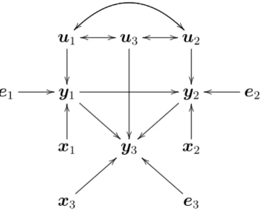
It is possible to express graphically the multiple trait animal model (MTAM) presented in equation (2.34). For example, in Rosa and Valente (2014) the authors show a graph as an example taking into account three traits, which can be seen in Figure 2.1.

b1 } } !! w

w ''

b2

w

w ''

b3

y₁ y₂ y₃

ε₁

O

O

a

a ε2 ==

O

O

g

g 77

7

7

g

g ε3

O

O

Figure 2.1 – Multiple trait animal model expressed using a graphical method

It is possible to express the MME for multiple traits as

X′(E−1⊗I)X X′(E−1⊗I)Z

Z′(E−1⊗I)X Z′(E−1⊗I)Z+G−₀1⊗A−1

ˆ β ˆ b =

X′(E−1⊗I)y Z′(E−1⊗I)y

, (2.35)

using equation (2.7) as reference, the BLUP and BLUE ofβandbcan be obtained by solving

the MME for the above multiple traits above.

Under Bayesian inference context, the MTAM is very similar to the single trait model that were presented previously. The difference comes from the prior distributions assigned to the dispersion parameters, where instead of scaled inverse chi-squared distributions, Wishart distri-butions are applied instead.

Some studies involve repeated measurements related to the same trait, or traits with maternal effects. In these situations, extensions or variations of the animal models are applied, for the contexts of either single or multiple traits, as can be seen in (SORENSEN; GIANOLA, 2002; ROSA; VALENTE, 2014; HENDERSON, 1984; MRODE, 2005).

2.3 Causal inference

a method to search for causal structures and an application to European quails. Some of those relationships can be easily verified (and therefore easily accepted) using simple situations, as in Pearl (2009), like the relationship between switch position and the working status of a lamp or the fact of using a hose and having a wet roof.

However, other causal relationships can be harder to accept and to verify, such as the effi-ciency of a weight gain treatment, teaching techniques, pest control via pesticides, smoking and cancer, among many examples (FOX, 2006; FOX, 2008; FERRON and HESS, 2007; GREENE, 2011; DUNCAN; HALLER; PORTES, 1968). Also, for some situations the assumption of causal relations should be analyzed carefully, since external factors can exert some influence on more than one variable at the same time, leading to spurious causal relationship, such as the number of people using umbrellas and car accidents, in which case rainfall easily can be seen as a common factor for both variables.

In this sense to verify if causal statements can be considered true, it is possible to conduct an experiment and randomize the treatments of interest, but in some situations randomization it is not possible, for various reasons as for example

• Operational Issues: Due to financial or logistical reasons, e.g., an experiment is too ex-pensive or there is not enough time available to run the randomization properly.

• Ethical Problems: A common problem related to research developed in medical science, where the randomization cannot be done, for example when some treatments can be too risky for the patient (e.g., forcing a group of patients to smoke or eat a high-calorie diet)

• Observational Variables: Variables that can be observed, but not externally defined, in which cases the randomization is impossible to perform, for instance gender, number of offspring and gestation length

These situation cited above can often occur and even though several studies concerning on explaining causal relationship among variables (e.g traits), usually are developed using tradi-tionally probabilistic models, that relates response variables to covariates (ROSA et al., 2011). In order explain these causal connections, causal inference methods were developed.

During the past fifty years this method has been widely used in different areas of human science, such as in studies related to economics, sociology and psychology. In economics sometimes there is interest in studying the market behavior in response to interventions, which usually are not performed randomly. In sociology and psychology causal studies have been used as a tool to explain many aspects of human behavior (BOLLEN, 1989; DUNCAN; HALLER; PORTES,1968; HAAVELMO, 1943; FOX, 2008).

association among the variables that do not reflect an effect, leading to spurious inferences. The well-known caveat is “Correlation does not imply causation” (PEARL, 2009; ROSA et al., 2011; ROSA; VALENTE, 2014; VALENTE et al. 2013).

Many other examples of common effects can be given besides the umbrella use and car accident case. For instance, a correlation exists between the shoe size of primary school students and mathematics ability, but this does not mean children with big feet are better at calculating. The common cause is age: older students are more advanced in math and have bigger feet. For this reason, in studies related to causal modeling two aspects are extremely important to verify

i) How are the effects: The factors that are involved and how they are related to each other;

ii) How much: The magnitude of causal relationships among the factors.

In order to investigate the relationship structure between variables, graph analyses (GA) can be used. This method allows to searching for how variables are related to each order, as well as the direction of the relationships. To estimate the magnitude of those relationships, one can use structural equation models (SEM). These models are used to estimate how much each variable affects others. When there is no information regarding the causal connections, both methods should be used jointly, however when the researcher has an idea about the relationships, fitting SEM allows inferring the magnitude of causal relationships.

Some algorithms have been developed to find causal structures, such as Peter Clark (PC), inductive causation (IC) and others. All of them are based on information about dependence, in-dependence, conditional independence and conditional dependence to assume there is a relation among variables. The first method is already available in the open software R.

To estimate the effects, specific software, such as TETRAD and LISREL, and packages for the open software R, such as sem and lavaan, have been developed. TETRAD allows to sim-ulating data using a prior structure and estimating the coefficients related to structure as well, using maximum likelihood and other procedures (more information can be found in TETRAD manual). LISREL is a software developed by Jöreskog and Sörbom (1974) that uses the full information maximum likelihood as a procedure to estimate the coefficient based on latent struc-tural models (FOX, 2008; FOX, 2006).

References

BOLLEN, K.A..Structural Equations with latent Variables. New York:John Wiley Sons Inc. 1995. 528 p.

CASELLA, G.; GEORGE, E. I. Explaining the Gibbs Sampler. The American Statistician, New York, v. 46, p. 167-174, 1992.

CHAIBUB NETO, E.C; FERARRA, T.C.; ATTIE, A.D.; YANDELL, B.S.. Inferring causal phenotype networks from segregating populations. Genetics, Baltimore, v. 179, p. 1089-1100, 2008.

CHAIBUB NETO, E.; KELLER, M.P; ATTIE, A.D.; YANDELL, B.S.. Causal graphical models in systems genetics: A unified framework for joint inference of causal network and genetic architecture for correlated phenotypes. Annals Applied Statistic, Cleveland, v. 4, p. 320-339, 2010.

DUNCAN, O.D.; HALLER, A.O.; PORTES, A.. Peer influences on aspirations: A reinterpretation. American Journal of Sociology, Chicago, v. 74, p. 119-137, 1968.

FERRON, J.M.; HESS, M.R. Estimation in SEM: A concrete example. Journal of Educational and Behavioral Statistics, Washington, v. 32, p. 110-120, 2007.

FOX, J.. An introduction to structural equation modeling, curso para programa de Computação Científica, FIOCRUZ: Rio de Janeiro, Brasil , 2008. 138p.

FOX, J.. Structural equation modeling with the sem package in R.Structural equation modeling, Hillsdale, v. 13, p. 465-486, 2006.

GAMERMAN, D.; LOPES, H. F.Markov Chain Monte Carlo:stochastic simulation for Bayes inference. London: Chapman Hall, 2006. 323 p.

GELFAND, A.E. Gibbs Sampling. Journal of the American Statistical Association, Alexandria, v. 95, n. 452, p. 1300-1304, 2000.

GELFAND, A.E.; SMITH, A. F. M. Sampling-based approaches to calculating marginal densities. Journal of the American Statistical Association, Alexandria , v. 85, n. 410, p. 348-409, June, 1990.

GELMAN, A.; CARLIN, J. B.; STER, H. S.; RUBIN, D.B.Bayesian data analysis. Boca Raton: Chapman HAll/CRC, 2000. 526 p.

GEMAN, S.; GEMAN, D. Stochastic Relaxation, Gibbs Distributions and Bayesian

GILMOUR, A.R.; THOMPSON, R.; CULLIS, B.R. Average information reml: an efficient algorithm for variance parameter estimation in linear mixed models.Biometrics, Arlington, v. 51, n. 4, p. 1440-1450, 1995.

GREENE, W.H..Econometric analysis, 7 ed. New York: Macmillan. 2011. 1232 p.

HAAVELMO, T.. The statistical implications of a system of simultaneous equations. Econometrica, London, v. 11, 1943.

HARVILLE, D.A. Maximum Likelihood Approaches to Variance Component Estimation and to Related Problems.Journal of the American Statistical Association, Alexandria, v. 72, n. 358, p. 320-338, Jun 1977.

HASTINGS,W. K. Monte Carlo Sampling methods using Markov chains and their application. Biometrika, London, v. 57, n. 1, p. 97-109, 1970.

HENDERSON, C.R.Applications of Linear Models in Animal Breeding. Ontario: University of Guelph, 1984. 462 p.

HENDERSON, C.R.. Best linear unbiased estimation and prediction under a selection model. Biometrics, Alexandria, v. 31, p. 423-447, 1975.

HENDERSON, C.R. and QUAAS, R.L.. Multiple trait evaluation using relatives records. Journal of Animal Science, Champaign, v. 43, p. 1188-1197, 1976.

HENDERSON, C.R.; KEMPTHORNE, O.; SEARLE, S.R.; VON KROSIGK, C.N.

Estimation of environmental and genetic trends from records subject to culling.Biometrics, Alexandria, v. 15, p. 192-218, 1959.

JEFREYS, H.Theory of probability. Oxford: Clarendon Press, 1961. 447 p.

JÖRESKOG, K.G.; SÖRBOM, D.LISREL 8.8 for Windows [Computer software]. Skokie, IL: Scientific Software International, Inc.

METROPOLIS, N.; ROSEMBLUT, A. W.; ROSEMBLUT, M.N. ; TELLER, A. H.; TELLER , E. Equation of state calculations by fast computing machines. Journal of Chemical Physics, New York, v. 21, p. 1987-1092, 1953

MRODE, R. A..Linear Models for the Prediction of Animal Breeding Values, 2 ed. Wallingford, Oxon, UK: CAB International, 2005. 344 p.

PAULINO, C.D.; TURKMAN, M. A.; MURTEIRA, B.Estatística Bayesiana. Lisboa: Fundação Calouste Gulbenkian, 2003. 446 p.

PATTERSON, H.D.; THOMPSON, R. Recovery of inter-block information when blocks sizes are unequal.Biometrika, Oxford, v. 58, n. 3, p. 545-554, 1971.

PEARL, J.Causality Models, Reasoning and inference. 2 ed. Cambridge, RU: Cambridge University, 2009. 484 p.

PINHEIRO, J.C.; BATES, D.M..Mixed-Effects Models in S and S-PLAS. New York: Springer, 2000. 528 p.

R. Development Core Team. R Foundation for Statistical Computing. R 2.15.2: A language and environment for statistical computing, Vienna, 2012. Avaiable in

<http://www.r-project.org/>. Acesso em: 23 nov. 2012

ROSA, G. J. M.; VALENDE, B. D.. Structural Equation Models for Studying Causal Phenotype Networks in Quantitative Genetics IN: SINOQUETE, C.; MOURAD, R.. Probabilistic Graphical Models for Genetics, Genomics and Postgenomics, Oxford University Press, 2014. 480 p.

ROSA, G.J.M.; VALENTE, B.D.; CAMPOS, G. de los; WU, X.L.; GIANOLA, D.; SILVA, M.A.. Inferring causal phenotype networks using structural equation models.Genetics Selection Evolution, London, v. 43, p. 1046-1057, 2011.

SCHAEFFER, L.R. Sire and cow evaluation under multiple trait models. Journal of Dairy Science, Champaing, v.67, p.1567-1580, 1984.

SORENSEN, D,; GIANOLA, D. Likelihood.Bayesian and MCMC methods in quantitative genetics. New York: Springer, 2002. 740 p.

The TETRAD Project Causal Models and Statistical Data. tetrad. Avaiable in

<http://www.phil.cmu.edu/projects/tetrad/current.html>. Acess in: 23 nov. 2012

VALENTE, B.D.; ROSA, G.J.M. Mixed effects structural equation models and phenotypic causal networks.Methods in molecular biology, Totowa, v. 1019, 449-564, 2013.

VALENTE, B.D.; ROSA, G.J.M.; CAMPOS, G. de los; GIANOLA, D.; SILVA, M.A.. Searching for recursive causal structures in multivariate quantitative genetics mixed models. Genetics, Baltimore, v. 185, p. 633-644, 2010.

VALENTE, B.D.; ROSA, G.J.M.; GIANOLA, D.; WU, X-L; WEIGEL. K.. Is Structural Equation Modeling Advantageous for the Genetic Improvement of Multiple Traits?Genetics, Baltimore, v. 194, p. 561-572, 2013.

VALENTE, B.D.; MOROTA, G.; PEÑAGARICANO, F., GIANOLA, D.; WEIGEL, K.; ROSA, G.J.M.. The causal meaning of genomic predictors and how it affects construction and comparison of genome-enabled selection models.Genetics, Baltimore, v. 200, 2015.

VALENTE, B.D.; ROSA, G.J.M.; SILVA, M.A.; TEIXEIRA, R.B.; TORRES, R.A.. Searching for phenotypic causal networks involving complex traits: an application to European quails. Genetics, Selection, Evolution, London, v. 43, p. 37-48, 2011.

3 ADVANTAGES OF USING HIGHER POLYNOMIAL

POLYNOMIAL INSTEAD OF LINEAR RELATIONSHIP

BETWEEN TRAITS IN STRUCTURAL EQUATION MODELS IN

QUANTITATIVE GENETICS: A SIMULATION STUDY

Abstract

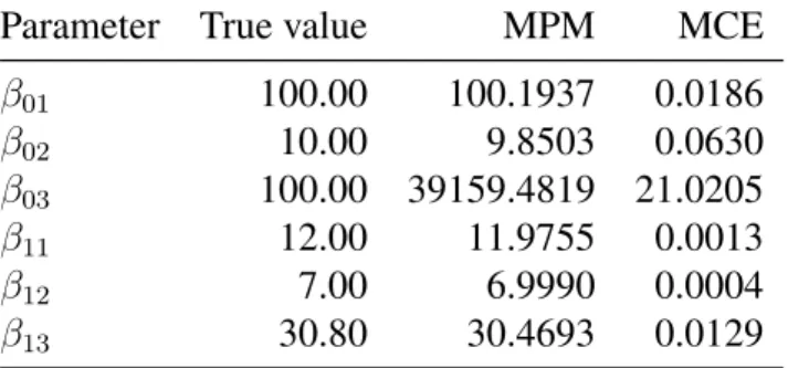
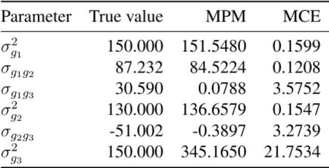
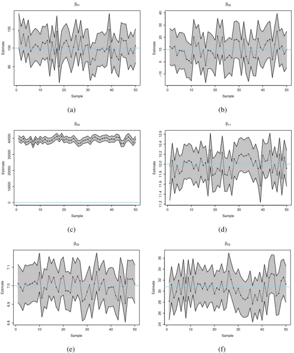
The concept of causality has been used in many studies in different areas of knowledge and its application has been growing during the past decade. Scientific investigation in biology generally involves learning causal relationships among variables, which are important in order to predict the consequences of interventions in the system. In quantitative genetics, so far, the most common approach to solve problems involving causality is assuming linear relationships between traits. However, such formulations are not suitable for scenarios where evidences of non linear relationships between traits can be observed. To overcome this limitation, this work proposes the use of polynomial mixed-effects structural equation model. In order to verify the advantages of the polynomial approach, a simulation study with 50 data sets was performed. Data was sampled from a fully recursive causal structure involving 3 traits, considering linear and non linear relationships between traits with one exogenous covariates associated to each endogenous trait. The Gibbs sampler was used to obtain posterior samples of model parame-ters and other unknowns. The standard linear model and a model accounting for second degree polynomials were compared. The results show that the inclusion of an extra polynomial de-gree enhances the SEM expressive power. For some situations the inappropriate assumption of linearity results in poor predictions of overall genetic effects, either by overestimating, underes-timating or even suggesting an opposite directions for them. The results also shows that there is no loss when using polynomial approach, because when the relationships were assumed linear the model estimate values equal o zero for the quadratic term.

Keywords: Structural models; causal inference; quantitative genetics; polynomial regression; Bayesian inference, Gibbs sampling

3.1 Introduction

Human beings typically try to comprehend the causal relationships among mensurable vari-ables in many different contexts. From as simple and obvious as using a hose and wetting the floor, to a more complex as the fact that smoking can be a cause of cancer or some more subjective examples as how intelligence affects career success, where the response can-not be measured (PEARL, 2009).

were developed to tackle limitations in such cases .

There are two fundamental aspects to be learned in the application of causal models to study the relationships among a set of variables , and there are two distinct methods for learn-ing each aspect: Graph analysis (GA) and structural equation modellearn-ing (SEM). While GA involves searching for causal structures that qualitatively represent how variables are causally connected, fitting SEM with a known causal structure allows inferring the magnitude of causal relationships. The latter involves a model that can be expressed as a multiple-trait regression model where some response variables may be considered as covariates in the right hand side of equations for other response variables (ROSA et al., 2011; LEE; ZHU, 2000; VALENTE et al., 2013; LEE; TANG, 2006).

During the past decades the number of studies involving causal models has been increased in many fields of scientific investigation. In biology, due to the complexity networks that ex-press the relationship among traits, the concept of causality can present some extra difficulties (HOYER et al., 2008; ROSA et al., 2011; BLAIR, 2012; VALENTE et al., 2010; MATURANA et al., 2009; CHAIBUB NETO, 2010; CHAIBUB NETO et al., 2010; VALENTE et al., 2011; CHAIBUB NETO et al., 2008).

Scientific investigation in biology frequently involves learning causal relationships among traits, in these systems can be easily seen situations where phenotypic traits may exert effects among themselves (i.e. calf liability and gestation length) (ROSA et al., 2011; VALENTE et al., 2010, MATURANA et al., 2009). This investigation is important in order to predict the consequences of interventions in the system. In this context, methods for causal inference become important tools. Notwithstanding , these structures of relationship take in account a complex functional network that should be analyzed carefully, specifically in quantitative genetics applications where individuals are genetically related due to familial relationships, such dependencies should also be modeled in SEM (CHAIBUB NETO, 2008; ROSA et al., 2011; VALENTE et al., 2010; VALENTE et al., 2013; VALENTE et al., 2011; WU; HERINGSTAD; GIANOLA, 2010; MATURANA et al., 2009; LIU; FUENTE; HOESCHELE, 2008; CHAIBUB NETO, 2010; GONZÁLEZ-RODRÍGUEZ et al., 2014; XIONG; FANG, 2004; LI et al., 2006). To solve situations using the genetic covariance, Gianola and Sorense (2004) adapted the causal models to the mixed models context (VALENTE et al., 2013).

However, so far, most studies in SEM applied to quantitative genetics have assumed that relationships between traits are linear, which may be unrealistic for some cases as for example (MATURANA et al., 2008; GONZÁLEZ-RODRÍGUEZ et al., 2014; VARONA; SORENSEN, 2014; KÖNIG et al., 2008).