DOES THE FINANCIAL SYSTEM SUPPORT ECONOMIC GROWTH IN
TIMES OF FINANCIALISATION? EVIDENCE FOR PORTUGAL
Ricardo Barradas
Dezembro de 2019
WP n.º 2019/04
DOCUMENTO DE TRABALHO WORKING PAPER
DOES THE FINANCIAL SYSTEM SUPPORT ECONOMIC GROWTH IN
1TIMES OF FINANCIALISATION? EVIDENCE FOR PORTUGAL
Ricardo Barradas
*
WP n. º 2019/04
DOI: 10.15847/dinamiacet-iul.wp.2019.041. INTRODUCTION ... 3
2. LITERATURE REVIEW ON THE FINANCE-GROWTH NEXUS IN TIMES OF FINANCIALISATION ... 5
3. LINEAR AND NON-LINEAR MODELS OF ECONOMIC GROWTH ... 7
4. DATA ... 9 5. ECONOMETRIC METHODOLOGY ... 11 6. RESULTS ... 13 7. CONCLUSION ... 21 8. REFERENCES ... 23 9. APPENDIX ... 28
1 The authors thank the helpful comments and suggestions of Sérgio Lagoa and Sofia Vale. The usual
_____________________________________________________________________________________
DOES THE FINANCIAL SYSTEM SUPPORT ECONOMIC GROWTH IN
TIMES OF FINANCIALISATION? EVIDENCE FOR PORTUGAL
ABSTRACT
The purpose of this paper is the conduction of a time series econometric analysis in order to examine empirically the relationship between the financial system and economic growth in Portugal from 1977 to 2016. The Portuguese financial system has experienced a strong wave of privatisations, liberalisations and deregulations since the adhesion of Portugal to the European Economic Community in 1986, which has not favoured a sustained path of strong economic growth since then. The growth of the financial system played even a crucial role in the recent sovereign debt crisis in Portugal, casting doubts on the conventional hypothesis on the finance-growth nexus. The paper estimates a linear finance-growth model and a non-linear finance-growth model, which includes four proxies for the financial system (money supply, credit, financial value added and stock market capitalisation) and four further control variables (inflation, government consumption, trade openness and education). The paper finds a negative linear relationship between the banking system and Portuguese economic growth, a positive linear relationship between the stock markets and Portuguese economic growth, a concave quadratic relationship between the banking system and Portuguese economic growth, and a convex quadratic relationship between the stock markets and Portuguese economic growth. This suggests that Portuguese policy makers should canalise efforts to decrease the importance of banking system and to increase the importance of stock markets in order to support more robust economic growth in the coming years.
KEYWORDS
Financial System, Economic Growth, Portugal, Time Series, Autoregressive Distributed Lag Estimator
JEL CLASSIFICATION
C32, E44, 016 and O47_____________________________________________________________________________________
1. INTRODUCTION
In 1986, Portugal joined the European Economic Community, which imposed the need to adopt a set of measures in order to achieve a higher development of the financial system. In the subsequent years, the Portuguese financial system suffered a strong transformation due to the widespread privatisations, liberalisations and deregulations of financial activities in order to fulfil the European rules. As a result, the financial system gained huge importance, which has not reflected a sustained path of strong economic growth in Portugal since that time. Moreover, the growth of the financial system is at the root of the last financial and economic crisis in Portugal, the so-called sovereign debt crisis (Barradas et al., 2018).
This process, typically referred as financialisation, emphasises a negative view of the financial system, casting doubts on the traditional hypothesis of the finance-growth nexus. These doubts have been fed by several empirical works that have concluded that there has been a weaning or even a reversal in the relationship between the financial system and economic growth (Rioja and Valev, 2004a and 2004b; Aghion et al., 2005; Kose et al., 2006; Prasad et al., 2007; Rousseau and Wachtel, 2011, Cecchetti and Kharroubi, 2012; Barajas et al., 2013; Dabla-Norris and Srivisal, 2013; Beck et al., 2014; Breintenlechner et al., 2015; Ehigiamusoe and Lean, 2018; Alexiou et al., 2018).
This paper conducts a time series econometric analysis in order to assess empirically the relationship between the financial system and economic growth in Portugal, by using annual data for 40 years from 1977 and 2016. This paper presents at least six novelties to the existing empirical literature. The first of these new additions is the analysis of the Portuguese context, for which the empirical evidence is non-existent. Portugal is a very interesting case study, mainly because the financial system has played an important role in the evolution of this economy and in the corresponding anaemic growth during recent years (Barradas et al., 2018). The second novelty is the application of a time series econometric analysis. In fact, the majority of empirical works on the finance-growth nexus performs cross-country analysis due to the higher available data (Ang, 2008). Time series econometric analysis offers several advantages in comparison with cross-country analysis and/or panel data econometric analysis, namely, by facilitating the comprehension of the historical, social and economic circumstances that are responsible for the economic growth over the time.The third novelty is the inclusion in our sample of periods of growth and of periods of recession. This is important because the nexus between the financial system and economic growth is too complex and is not stable over time (Grochowska et al., 2014). The fourth is the estimation of both linear and non-linear growth models, taking into account that the financial system exerts an inverted U-shaped effect on economic growth. The estimation of non-linear growth models is scarcer, despite the existence of several exceptions that have
_____________________________________________________________________________________ confirmed a concave quadratic relationship between the financial system and economic growth (Cecchetti and Kharroubi, 2012; Barajas et al., 2013; Dabla-Norris and Srivisal, 2013; Beck et
al., 2014). The fifth is the use of different proxies to assess the importance of the financial system
(money supply, credit, financial value added and stock market capitalisation). This allows us to take into consideration the different scopes of the financial system, such as their size, depth and efficiency (Beck et al., 2014; Breitenlechner et al., 2015). The sixth novelty is the inclusion of other control variables (inflation, government consumption, trade openness and education) in our growth models, which mitigates the problem of omitted relevant variables and favours more consistent and unbiased estimates (Wooldridge, 2003; Kutner et al., 2005; Brooks, 2009).
Our estimates will be produced using the Autoregressive Distributed Lag (ARDL) estimator, because our variables are a mixture of variables that are stationary in levels and variables that are stationary in first differences. Our linear results confirm that the financial (banking) system has been detrimental to Portuguese economic growth and that the financial (stock) markets have been beneficial to Portuguese economic growth. Our non-linear results confirm the existence of a concave quadratic relationship between money supply, credit and financial value added and Portuguese economic growth, and the existence of a convex quadratic relationship between stock market capitalisation and Portuguese economic growth. This implies the need to reduce the importance of the former three dimensions of the financial system (more connected with the banking system) and the need to increase the importance of the latter dimension (more linked with the stock markets) in order to achieve higher economic growth in the future.
This paper is structured as follows. Section 2 contains the literature review on the finance-growth nexus in times of financialisation. In Section 3, both linear and non-linear finance-growth models are presented. Variables, proxies and the respective sources are described in Section 4. The econometric methodology is explained in Section 5. Section 6 presents the long-term and short-term estimates for the linear and non-linear growth model. Finally, Section 7 concludes and discusses the main measures that should be adopted by Portuguese policy makers in order to sustain a higher level of economic growth in the coming years.
_____________________________________________________________________________________
2. LITERATURE REVIEW ON THE FINANCE-GROWTH NEXUS IN TIMES
OF FINANCIALISATION
The financial system has been subjected to strong liberalisation and deregulation since the 1970s and 1980s in the majority of developed economies, mainly as an excuse to support higher financial development and to boost economic growth (Barradas, 2016). Consequently, the financial system has experienced excessive growth since then by originating several deleterious consequences on economy and on society, such as the emergence of several financial crises, the lessened resilience of the banking system and the higher instability of the aggregate demand (Rousseau and Wachtel, 2011; Barajas et al., 2013; Dabla-Norris and Srivisal, 2013).
This harmful impact of the financial system on the economy and on society has normally been called as financialisation. The negative view of the financial system has also been confirmed by the emergence of several empirical works that cast doubts on the well-recognised hypothesis of the finance-growth nexus, because they have identified a weakening in the positive impact of the financial system on economic growth, or even a negative impact (Rioja and Valev, 2004a and 2004b; Aghion et al., 2005; Kose et al., 2006; Prasad et al., 2007; Rousseau and Wachtel, 2011, Cecchetti and Kharroubi, 2012; Barajas et al., 2013; Dabla-Norris and Srivisal, 2013; Beck et al., 2014; Breintenlechner et al., 2015; Ehigiamusoe and Lean, 2018; Alexiou et al., 2018). Against this backdrop, several scholars have stressed that the relationship between the financial system and economic growth is non-linear by behaving like a concave quadratic function. This shows that the financial system has an inverted U-shaped impact on economic growth, which means that the economic growth can decelerate with the rise of the financial system from a specific point (i.e. the turning point of the concave quadratic function). Effectively, the negative relationship between the financial system and economic growth found in the aforementioned empirical works occurs because the growth of the financial system has already surpassed the respective turning point in the countries.
The literature on this matter presents at least eight explanations for the weakening or the reversal in the impact of the financial system on economic growth in times of financialisation. The first explanation is related to the specific growth of the financial system, which has occurred essentially in activities (e.g. non-intermediation financial activities, like proprietary trading, market making, provision of advisory services, insurance, derivatives, securitisation, shadow banking and other non-interest income-generating activities) and/or in institutions (e.g. investment funds, money market funds, hedge funds, private equity funds, special purpose vehicles, among others) that do not directly favour a higher level of economic growth (Stockhammer, 2010; Lucarelli, 2012; Beck et al., 2014; Sawyer, 2014 and 2015). The second
_____________________________________________________________________________________ explanation is associated with the liquidity function of the financial system, which has been responsible for narrowing the linkage between savings and investments (Sawyer, 2014). Savers are simply increasing financial transactions to reorganise their portfolios, which do not necessarily generate more funds for investors. The third explanation pertains to the unstable and speculative nature of financial markets (Ang, 2008) in line with Minsky’s ‘financial instability hypothesis’ (1991), which tends to contribute to higher instability of the aggregate demand, and particularly of consumption and investment (Dabla-Norris and Srivisal, 2013). The fourth explanation is connected with the huge growth of credit and the corresponding indebtedness of economic agents (especially households, through mortgage credit) in times of financialisation, which have decreased the resilience of the banking system, increased the vulnerability of economies to any negative shocks and impaired the real and physical investments (Stockhammer, 2010; Lapavitsas, 2011; Orhangazi, 2008; Rousseau and Wachtel, 2011; van der Zwan, 2014). As emphasised by Boone and Girouard (2002), Stockhammer (2009) and Hein (2012), this strong growth of credit supply in times of financialisation was possible due to the rise of competition among banks, the emergence of new financial instruments (e.g. home equity loans and credit cards), financial innovation (e.g. debt securitisation and the ‘originate to distribute’ strategies of banks) and the low level of interest rates, which led to a deterioration of creditworthiness standards and led to credit being more available even for low-income and low-wealth households. This trend was also supported by the strong growth of credit demand by households, who incur debt in order to compensate for the decline of their wages in times of financialisation (Barradas and Lagoa, 2017a; Barradas, 2019). The fifth explanation relates to the risk-aversion behaviour practised by investors through excessive investments in tangible assets than can be used as collateral instead of investments in knowledge-based assets (that would be more growth-enhancing) that is encouraged by banks in order to maximise the likelihood of receiving the granted credits (Ang, 2008). This happens also because investors aim to satisfy impatient shareholders, who are more concerned with short-term profits rather than long-term expansion. As a result, investors invest more in tangible and/or in financial assets, which crowds out investments in real and/or knowledge-based activities (Barradas, 2017; Barradas and Lagoa, 2017b). The sixth explanation is connected to the resources’ absorption by the financial sector, which reduces the existing resources to the real and productive sectors (Cecchetti and Kharroubi, 2012; Sawyer, 2014). The seventh explanation relates to the other problems from the excessive growth of the financial system that are also detrimental for economic growth, like the imperfect competition between financial institutions, rent-seeking behaviour by economic agents, implicit insurance due to bailouts and negative externalities from auxiliary services (Beck et al., 2014). The eighth explanation corresponds to the recognition that the ‘supply leading hypothesis’ only
_____________________________________________________________________________________ occurs in the early stages of economic development, which suggests that the financial system does already not boost economic growth in the more developed economies (Alexiou et al., 2018).
This paper aims to address empirically the effect of the financial system on economic growth in times of financialisation by carrying out a time series econometric analysis for Portugal from 1977 to 2016. This paper contributes to the existing literature in six ways, namely, by focusing on Portugal; performing a time series econometric analysis; incorporating the pre-crisis period, the crisis period and the post-crisis period; estimating a linear and a non-linear relationship between the financial system and economic growth; incorporating several measures as proxies for the financial system; and including other traditional variables that are typically used in similar empirical works on that subject.
3. LINEAR AND NON-LINEAR MODELS OF ECONOMIC GROWTH
With the aim of addressing the effect of the financial system on economic growth, we estimate a linear growth model based on King and Levine’s (1993) version of the Barro (1991) growth regression, with the inclusion of a variable to capture the financial system, which takes the following form:
(1)
where t is the time period (years), Y is the growth rate of the real per capita gross domestic product2, X is a set of control variables that are recognised as important drivers of economic
growth, F is a proxy of the financial system and u is an independent and identically distributed (white noise) disturbance term with null average and constant variance (homoscedastic).
We also estimate a non-linear growth model taking into account the potential concave quadratic relationship between the financial system and economic growth (Cecchetti and Kharroubi, 2012; Barajas et al., 2013; Dabla-Norris and Srivisal, 2013; Beck et al., 2014), which takes the following form:
(2)
2 The advantage of using the growth rate of the real per capita gross domestic product instead of the growth
rate of the real gross domestic product as a proxy of economic growth is that this allows us to take into account not only the investors’ prospects, but also the people’s prosperity (Alexiou et al., 2018). Note also that the majority of the empirical studies on the relationship between the financial system and economic growth use the growth rate of the real per capita gross domestic product (Rioja and Valev, 2004a and 2004b; Rousseau and Wachtel, 2011; Hassan et al., 2011; Beck et al., 2014; Jedidia et al., 2014; Breitenlechner et al., 2015; Durusu-Ciftci et al., 2017; Ehigiamusoe and Lean, 2018; Alexiou et al., 2018).
_____________________________________________________________________________________ The non-linear growth model allows us to determine the turning point of the concave quadratic function. Until this point, there has been a positive relationship between the financial system and economic growth. From this point, there is a negative relationship between the financial system and economic growth. The turning point – F* – is obtained by determining the maximum of the concave quadratic function through the estimated coefficients, i.e.:
(3)
In the linear growth model and in the non-linear growth model, our control variables are the inflation rate, general government consumption, the degree of trade openness and the education level of the population. Note that the majority of empirical works on the relationship between the financial system and economic growth use similar control variables (Rioja and Valev, 2004a and 2004b; Rousseau and Wachtel, 2011; Hassan et al., 2011; Beck et al., 2014; Jedidia et al., 2014; Breitenlechner et al., 2015; Durusu-Ciftci et al., 2017; Ehigiamusoe and Lean, 2018; Alexiou et
al., 2018), which facilitates the comparison of our results with these empirical works.
The inflation rate has an expected negative effect on economic growth due to the uncertainty and the corresponding decrease of savings, investment and capital accumulation in times of higher levels of inflation (Fischer, 1993; Barro, 2003). In addition, higher levels of inflation are associated with lessened institutional development, which by itself constrains economic growth (Schnabl, 2009; Alexiou et al., 2018).
General government consumption is expected to exert a positive effect on economic growth, which rests on the (short-term) Keynesian theory that economic growth can be boosted with a higher level of public expenditure (Arestis and Sawyer, 2005; Alexiou and Nellis, 2013; Ehigiamusoe and Lean, 2018; Alexiou et al., 2018).
Economic growth also depends positively on the degree of trade openness due to the positive effects of trade openness on competition and technological progress (Winters, 2004; Ehigiamusoe and Lean, 2018; Alexiou et al., 2018).
The education level of the population has an expected positive impact on economic growth, which translates into the positive effect that human capital has on economic growth (Rousseau and Wachtel, 2011; Ehigiamusoe and Lean, 2018).
_____________________________________________________________________________________
4. DATA
Annual data for Portugal was collected from 1977 and 2016, covering a total of 40 observations. This corresponds to the time span and periodicity for which data for all variables under study are available. Effectively, the proxy of stock market capitalisation is only available after 1977, and the proxy of money supply is only available until 2016. However, our time span covers the times in which financialisation became more notorious in Portugal, which has occurred since the mid-1980s with privatisations, liberalisations and deregulations of the Portuguese financial system in line with the European rules and the ongoing integration process during that time (Barradas et al., 2018).
According to other empirical works on the relationship between the financial system and economic growth, we use four different proxies to measure the importance of the financial system, namely money supply (Rioja and Valev, 2004a and 2004b; Hassan et al., 2011; Rousseau and Wachtel, 2011; Breitenlechner et al., 2015; Ehigiamusoe and Lean, 2018; Alexiou et al., 2018), credit (Rioja and Valev, 2004a and 2004b; Hassan et al., 2011; Rousseau and Wachtel, 2011, Cecchetti and Kharroubi, 2012; Beck et al., 2014; Jedidia et al., 2014; Breitenlechner et al., 2015; Durusu-Ciftci et al., 2017; Ehigiamusoe and Lean, 2018; Alexiou et al., 2018); financial value added (Beck et al., 2014); and stock market capitalisation (Alexiou et al., 2018). The use of these different proxies is a very common empirical strategy, namely due to the recognition that ‘defining appropriate proxies for the degree of financial development is, indeed, one of the challenges faced by empirical researchers’ (Edwards, 1996: 21). This allows us to reflect in a more complete way on the role of financial system, namely by encompassing proxies related to the banking system and a proxy related to financial markets that simultaneously assess its size, depth and efficiency (Beck et al., 2014; Breitenlechner et al., 2015). Money supply, credit and financial value added are more directly related with the banking system, whereas the stock market capitalisation is more connected with the financial (stock) markets.
Proxies and sources for each variable under study are presented in Table 1. Table 2 exhibits the descriptive statistics for each variable, Table 3 contains the correlations between them, and Figure A1 in the Appendix illustrates the respective plots. Note that all the correlations between the variables linked with financial system and economic growth are negative, which seems to suggest that the increasing trend in the financial system in Portugal since 1977 has not been accompanied by a positive path on economic growth (Figure A1 in the Appendix)3. This
3 We recognise that some correlations seem to indicate the presence of multicollinearity, mainly because
some of them are higher than the traditional ceiling of 0.8 in absolute figures (Studenmund, 2005). Nevertheless, this hypothesis is rejected through the calculation of variance inflation factors, because they are lower than the traditional ceiling of 10 (Kutner et al., 2004). Results are available upon request.
_____________________________________________________________________________________ seems to indicate that the hypothesis of the finance-growth nexus has not occurred in Portugal in recent decades.
Table 1 – The proxies and sources of each variable
Variable Proxy Source
Economic Growth GDP per capita growth (annual %) World Bank
Inflation Inflation, consumer prices (annual %) World Bank
Government Consumption General government final consumption expenditure (% of GDP) World Bank
Trade Openness Exports and imports of goods and services (% of GDP) World Bank
Education Actual schooling rate, upper-secondary education (%) PORDATA
Money Supply Liquid liabilities (% of GDP) Fred St. Louis
Credit Total credit to private non-financial sector (% of GDP) Fred St. Louis
Financial Value Added Gross value added of financial, insurance and real estate activities (% of total) PORDATA
Stock Market Capitalisation Stock market capitalization (% of GDP) Fred St. Louis
Table 2 – The descriptive statistics of each variable
Variable Mean Median Maximum Minimum Standard
Deviation Skewness Kurtosis
Economic Growth 0.019 0.018 0.076 -0.036 0.026 -0.080 2.694 Inflation 0.086 0.039 0.310 -0.008 0.087 1.030 2.913 Government Consumption 0.170 0.178 0.214 0.121 0.030 -0.324 1.665 Trade Openness 0.628 0.624 0.802 0.405 0.090 -0.119 3.480 Education 0.448 0.561 0.753 0.089 0.234 -0.311 1.517 Money Supply 0.845 0.839 1.015 0.583 0.108 -0.456 2.658 Credit 1.430 1.305 2.315 0.785 0.494 0.346 1.665
Financial Value Added 0.138 0.135 0.181 0.097 0.027 0.146 1.851
Stock Market
Capitalisation 0.219 0.224 0.512 0.003 0.165 0.082 1.771
Table 3 – The correlations between variables
EC I GC TO E MS C FVA SMC EC 1.000 I 0.171 1.000 GC -0.424*** -0.880*** 1.000 TO -0.227 -0.663*** 0.587*** 1.000 E -0.373** -0.917*** 0.920*** 0.742*** 1.000 MS -0.559*** -0.737*** 0.794*** 0.795*** 0.834*** 1.000 C -0.620*** -0.542*** 0.691*** 0.655*** 0.724*** 0.839*** 1.000 FVA -0.420*** -0.790*** 0.833*** 0.727*** 0.905*** 0.771*** 0.812*** 1.000 SMC -0.151 -0.826*** 0.858*** 0.616*** 0.833*** 0.701*** 0.638*** 0.726*** 1.000 Note: *** indicates statistical significance at 1% level, ** indicates statistical significance at 5% level and * indicates statistical significance at 10% level
Table 4 – P-values of the ADF unit root test
Variable
Level First Difference
Intercept Trend and
Intercept None Intercept
Trend and Intercept None Economic Growth 0.037 0.139* 0.443 0.000 0.000 0.000* Inflation 0.261 0.954 0.002* 0.005 0.000* 0.000 Government Consumption 0.465* 0.996 0.936 0.000 0.027 0.000* Trade Openness 0.274 0.125* 0.948 0.000* 0.053 0.000 Education 0.833 0.575 0.874* 0.110* 0.067 0.053 Money Supply 0.079 0.034* 0.962 0.001* 0.004 0.000 Credit 0.018 0.328* 0.679 0.069 0.238 0.007*
Financial Value Added 0.911 0.012* 0.961 0.004* 0.023 0.109
Stock Market Capitalisation 0.554* 0.976 0.712 0.001 0.003 0.000*
Money Supply2 0.542 0.049* 0.946 0.001* 0.003 0.000
Credit2 0.009* 0.232 0.556 0.037 0.144 0.003*
Financial Value Added2 0.934 0.122* 0.968 0.000 0.057 0.121*
Stock Market Capitalisation2 0.612* 0.936 0.511 0.001 0.002 0.000*
Note: The lag lengths were selected automatically based on the AIC criteria and * indicates the exogenous variables included in the test according to the AIC criteria
_____________________________________________________________________________________
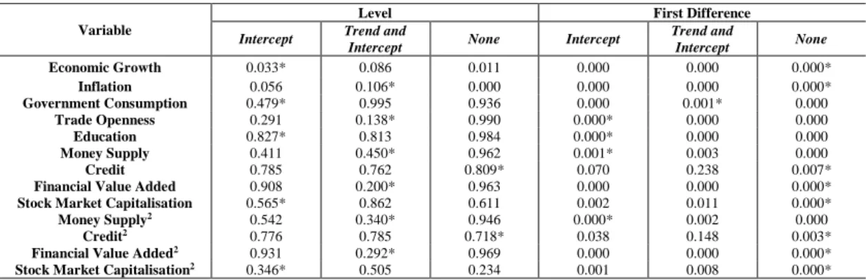
Table 5 – P-values of the PP unit root test
Variable
Level First Difference
Intercept Trend and
Intercept None Intercept
Trend and Intercept None Economic Growth 0.033* 0.086 0.011 0.000 0.000 0.000* Inflation 0.056 0.106* 0.000 0.000 0.000 0.000* Government Consumption 0.479* 0.995 0.936 0.000 0.001* 0.000 Trade Openness 0.291 0.138* 0.990 0.000* 0.000 0.000 Education 0.827* 0.813 0.984 0.000* 0.000 0.000 Money Supply 0.411 0.450* 0.962 0.001* 0.003 0.000 Credit 0.785 0.762 0.809* 0.070 0.238 0.007*
Financial Value Added 0.908 0.200* 0.963 0.000 0.000 0.000*
Stock Market Capitalisation 0.565* 0.862 0.611 0.002 0.011 0.000*
Money Supply2 0.542 0.340* 0.946 0.000* 0.002 0.000
Credit2 0.776 0.785 0.718* 0.038 0.148 0.003*
Financial Value Added2 0.931 0.292* 0.969 0.000 0.000 0.000*
Stock Market Capitalisation2 0.346* 0.505 0.234 0.001 0.008 0.000*
Note: * indicates the exogenous variables included in the test according to the AIC criteria
Table 4 and Table 5 contain the results of the traditional augmented Dickey and Fuller (1979) (ADF) unit root test and the Phillips and Perron (1998) (PP) unit root test for each variable. As we will estimate both linear and non-linear growth models, we also present the results of the ADF and PP tests for the squared terms of the variables linked to the financial system. At the conventional significance levels, we conclude that we have a mixture of variables that are integrated of order zero and variables that are integrated of order one by both unit root tests. Education and of the squared term of financial value added are the only exceptions according to the ADF test, although they are definitively integrated of order one by the PP test.
5. ECONOMETRIC METHODOLOGY
Our growth models will be estimated using the ARDL estimator proposed by Pesaran (1997), Pesaran and Shin (1999) and Pesaran et al. (2001). This is the more reliable estimator when we are in the presence of variables that are stationary in levels and variables that are stationary in the first differences. This estimator produces unbiased and consistent estimates, even in the case of small and finite samples and/or when there are endogenous variables among the independent variables (Pesaran and Smith, 1998). The issue of endogeneity on the empirical analysis on the finance-growth nexus should be taken into account due to the theoretical claims on the existence of a potential bi-causality between financial system and economic growth in line with the
‘demand-following hypothesis’ and ‘supply leading hypothesis’ (Alexiou et al., 2018). We will produce the respective estimates in the EViews software (version 10).
_____________________________________________________________________________________ The implementation of the ARDL estimator involves four different stages. Firstly, we determine the number of lags to be included in our estimates following the results of the different information criteria. This is relevant by taking into account that the ARDL estimator explains the behaviour of the dependent variable through the lagged values of itself and with the contemporaneous and the lagged values of the independent variables. Secondly, we determine if there is a cointegration relationship between our variables through the bounds test methodology developed by Pesaran et al. (2001). Thirdly, we perform a set of diagnostic tests in order to assess the reliability of our estimates. Five different diagnostic tests will be presented, namely, to assess if the residuals are not serially correlated (through the Breusch-Godfrey Serial Correlation LM test), are normal (through the Jarque-Bera test) and are homoscedastic (through the Breusch-Pagan-Godfrey test), to assess if our models are well specified in their functional forms (through Ramsey’s RESET test) and to assess the stability of our estimates and the absence of potential structural breaks (through the CUSUM test). If our models fail in at least one of these diagnostic tests, we need to adopt several remedies in order to resolve the problems and ensure the reliability of our estimates. Fourthly, we present the long-term estimates and the short-term estimates of our growth models. As we are modelling the economic growth that does not seem to have any intercept and/or trend in its evolution (Figure A1 in the Appendix), our estimates will take into account the first trend specification (i.e. the so-called ‘none’).
_____________________________________________________________________________________
6. RESULTS
As we already mentioned in the previous section, the first step is the determination of the number of lags according to the different information criteria (Table 6)4. The choice of the optimal number
of lags to be incorporated in each model is defined according to the majority of the information criteria, which are four for all models. The only exceptions are the linear growth model with the proxy of credit, the non-linear growth model with the proxy of money supply and the non-linear growth model with the proxy of credit, for which the optimal number of lags is three, three and two, respectively. It is worth to noting that EViews software automatically defines the number of lags to be incorporated in each model up to the specified maximum.
Table 6 – Values of the information criteria by lag
Growth Model
Proxy (Financial System) Lag LR FPE AIC SC HQ
Linear Growth Model Money Supply 0 n.a. 5.42e-18 -22.729 -22.465 -22.637 1 263.585 4.66e-21 -29.818 -27.970* -29.174 2 50.442 4.57e-21 -30.012 -26.581 -28.814 3 50.863 2.81e-21 -31.003 -25.989 -29.253 4 59.085* 3.322e-22* -34.375* -27.777 -32.072*
Linear Growth Model Credit
0 n.a. 1.74e-16 -19.262 -19.000 -19.169
1 339.179 1.54e-20 -28.622 -26.793* -27.977
2 54.600 1.30e-20 -28.951 -25.555 -27.753
3 51.329* 8.32e-21* -29.856* -24.893 -28.106*
Linear Growth Model Financial Value Added
0 n.a. 1.91e-19 -26.074 -25.810 -25.982
1 286.782 7.39e-23 -33.963 -32.115* -33.318
2 54.873 5.98e-23 -34.348 -30.918 -33.151
3 31.464 1.15e-22 -34.199 -29.185 -32.449
4 62.025* 1.04e-23* -37.838* -31.240 -35.535*
Linear Growth Model Stock Market Capitalisation
0 n.a. 2.02e-17 -21.415 -21.151 -21.322
1 272.971 1.26e-20 -28.827 -26.980* -28.183
2 66.902 6.02e-21 -29.736 -26.305 -28.539
3 35.411 9.20e-21 -29.819 -24.805 -28.069
4 60.671* 9.39e-22* -33.335* -26.737 -31.032*
Non-Linear Growth Model Money Supply Money Supply2 0 n.a. 2.59e-22 -29.841 -29.537 -29.734 1 299.863 1.24e-25 -37.533 -35.095* -36.673 2 71.101 9.32e-26 -38.116 -33.544 -36.504 3 71.937* 2.72e-26* -40.263* -33.558 -37.899*
Non-Linear Growth Model Credit Credit2
0 n.a. 6.99e-18 -19.637 -19.335 -19.530
1 420.634 7.85e-23 -31.079 -28.666* -30.220*
2 67.981* 7.07e-23* -31.456* -26.931 -29.846
Non-Linear Growth Model Financial Value Added Financial Value Added2
0 n.a. 2.40e-26 -39.128 -38.820 -39.021
1 351.589 1.35e-30 -48.963 -46.500 -48.103
2 71.182 9.61e-31 -49.630 -45.012 -48.018
3 61.012 5.17e31 -51.266 -44.492 -48.902
4 107.246* 3.26e-35* -63.865* -54.935* -60.748*
Non-Linear Growth Model Stock Market Capitalisation Stock Market Capitalisation2
0 n.a. 3.69e-21 -27.185 -26.877 -27.077
1 290.916 1.82e-24 -34.852 -32.389 -33.992
2 87.839 5.84e-25 -36.313 -31.694 -34.701
3 64.475 2.45e-25 -38.196 -31.422 -35.832
4 117.042* 3.82ee-30* -52.194* -43.265* -49.077* Note: * indicates the optimal lag order selected by the respective information criteria
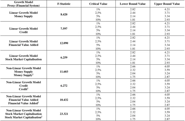
The second stage is the analysis of whether there is a cointegration relationship between variables under study through the bounds test methodology (Table 7). We strongly confirm that our
4 For the majority of models, we put into consideration a number of lags between zero and four, as the
unrestricted VAR does not satisfy the stability condition with a higher number of lags because at least one characteristic polynomial root would be outside the unit circle (Lütkepohl, 1991). For the linear growth model with the proxy of credit and the non-linear growth model with the proxy of money supply, a number of lags between zero and three were put into consideration, and for the non-linear growth model with the proxy of credit, a number of lags between zero and two were considered in order to guarantee the aforementioned stability condition, which would not be fulfilled if we had used a higher number of lags.
_____________________________________________________________________________________ variables are cointegrated because the computed F-statistics are higher than the upper-bound critical values for all linear and non-linear growth models.
Table 7 – Bounds test for cointegration analysis
Growth Model
Proxy (Financial System) F-Statistic Critical Value Lower Bound Value Upper Bound Value Linear Growth Model
Money Supply 8.420
1% 2.82 4.21
2,5% 2.44 3.71
5% 2.14 3.34
10% 1.81 2.93
Linear Growth Model Credit 7.597 1% 2.82 4.21 2,5% 2.44 3.71 5% 2.14 3.34 10% 1.81 2.93
Linear Growth Model
Financial Value Added 12.090
1% 2.82 4.21
2,5% 2.44 3.71
5% 2.14 3.34
10% 1.81 2.93
Linear Growth Model
Stock Market Capitalisation 6.259
1% 2.82 4.21
2,5% 2.44 3.71
5% 2.14 3.34
10% 1.81 2.93
Non-Linear Growth Model Money Supply Money Supply2 11.603 1% 2.66 4.05 2,5% 2.32 3.59 5% 2.04 3.24 10% 1.75 2.87
Non-Linear Growth Model Credit Credit2 6.272 1% 2.66 4.05 2,5% 2.32 3.59 5% 2.04 3.24 10% 1.75 2.87
Non-Linear Growth Model Financial Value Added Financial Value Added2
10.432
1% 2.66 4.05
2,5% 2.32 3.59
5% 2.04 3.24
10% 1.75 2.87
Non-Linear Growth Model Stock Market Capitalisation Stock Market Capitalisation2
23.321
1% 2.66 4.05
2,5% 2.32 3.59
5% 2.04 3.24
10% 1.75 2.87
In the third step, we conduct a set of diagnostic tests (Table 8). We can confirm that the linear growth models with the proxies of money supply and stock market capitalisation and the non-linear growth model with the proxy of credit do not suffer from any econometric problems. For these three models, we can ensure that the respective residuals are not serially correlated and they are normal and homoscedastic, and we can also guarantee that these three models are well specified in their functional forms. The remaining five models present several econometric problems, and therefore we need to adopt some remedies to ensure the reliability of our estimates. For the linear growth model with the proxy of credit and for the non-linear growth model with the proxy of stock market capitalisation, we reject the null hypothesis that residuals are homoscedastic. Therefore, we will proceed by taking into account the Newey-West estimator to produce the final estimates of these two models. The adoption of this remedy does not modify the conclusion for the remaining diagnostic tests. The conclusion that residuals are normal is rejected for the linear growth model with the proxy of financial value added. Nonetheless, we will not adopt any remedy for this model, as the central limit theoremensures that our residuals are indeed normal due to the presence of a sample with more than 30 observations. In addition, and as recognised by Hendry and Juselius (2000), the normality hypothesis is seldom satisfied in economic applications, which does not invalidate the global robustness of estimates or the
_____________________________________________________________________________________ respective statistical inference. The hypothesis that the model is well specified in its functional form is rejected for the non-linear growth model with the proxy of money supply. As a remedy, we will use a number of lags equal to one (instead of three or even two)5. With only one lag, the
hypothesis that this model is well specified in its functional form cannot be rejected, and the model passes in all the remaining diagnostic tests. For the non-linear growth model with the proxy of financial value added, we reject the hypotheses on the right functional form and on the absence of serial correlation of the residuals. Thus, we change the number of lags to three, and we use the Newey-West estimator. With these two remedies, the remaining diagnostic tests were also confirmed, and no further econometric problems occur. Finally, for all eight models, the CUSUM tests6 confirm the stability of our estimates and the absence of any structural breaks. After
confirming that our models do not suffer from any econometric problems and/or after introducing the remedies to correct those problems, we can advance to the fourth and final stage by presenting our results.
Table 8 – Diagnostic tests for ARDL estimates
Growth Model
Proxy (Financial System) Diagnostic Test F-Statistic P-value
Linear Growth Model Money Supply
Breusch-Godfrey 1.145 0.326
Jarque-Bera 1.048 0.592
Breusch-Pagan-Godfrey 0.817 0.677
Ramsey’s RESET 2.247 0.185
Linear Growth Model Credit
Breusch-Godfrey 0.094 0.762
Jarque-Bera 0.074 0.964
Breusch-Pagan-Godfrey 2.764 0.017
Ramsey’s RESET 0.447 0.510
Linear Growth Model Financial Value Added
Breusch-Godfrey 1.342 0.269
Jarque-Bera 6.530 0.038
Breusch-Pagan-Godfrey 0.843 0652
Ramsey’s RESET 2.547 0.137
Linear Growth Model Stock Market Capitalisation
Breusch-Godfrey 0.022 0.884
Jarque-Bera 1.584 0.453
Breusch-Pagan-Godfrey 1.416 0.270
Ramsey’s RESET 0.364 0.558
Non-Linear Growth Model Money Supply Money Supply2 Breusch-Godfrey 0.492 0.494 Jarque-Bera 1.137 0.566 Breusch-Pagan-Godfrey 0.607 0.857 Ramsey’s RESET 11.407 0.005
Non-Linear Growth Model Credit Credit2 Breusch-Godfrey 0.534 0.471 Jarque-Bera 2.884 0.237 Breusch-Pagan-Godfrey 1.506 0.189 Ramsey’s RESET 0.406 0.529
Non-Linear Growth Model Financial Value Added Financial Value Added2
Breusch-Godfrey 16.792 0.026
Jarque-Bera 0.308 0.857
Breusch-Pagan-Godfrey 0.759 0.714
Ramsey’s RESET 9.193 0.056
Non-Linear Growth Model Stock Market Capitalisation Stock Market Capitalisation2
Breusch-Godfrey 4.348 0.172
Jarque-Bera 0.337 0.845
Breusch-Pagan-Godfrey 37.111 0.027
Ramsey’s RESET 0.249 0.667
Note: Breusch-Godfrey tests were conducted with 1 lag and Ramsey’s RESET tests were performed with 1 fitted term, albeit results do not change if we had used more lags and more fitted terms, respectively
5 Note that if we use two lags the hypothesis that the model is well specified in its functional form is also
rejected. Results are available upon request.
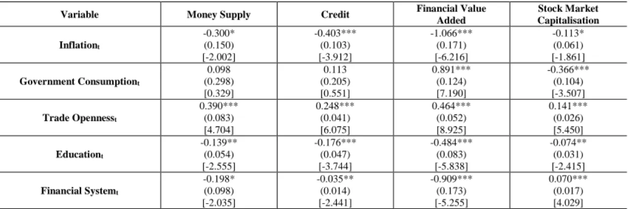
_____________________________________________________________________________________ With regard to the linear growth models and the corresponding long-term estimates (Table 9), we conclude that all variables are statistically significant and have the expected signs. The only exceptions pertain to the variables of government consumption and education. The former is statistically insignificant in the model with the proxies of money supply and credit and statistically significant in the other two models. In the model with the proxy of financial value added, government consumption has the expected positive sign by confirming the (short-term) Keynesian argument that higher government spending boosts economic growth. However, this result is not corroborated by the model with the proxy of stock market capitalisation, according to which government spending is detrimental to economic growth. This negative relationship could be attributable to high public sector wages, inflation pressures, inefficient public corporations, corruption and other phenomenon that tend to impair economic growth (Alexiou et
al., 2018). A similar result was found by Rioja and Valev (2004a and 2004b), Hassan et al. (2011),
Rousseau and Wachtel (2011), Cecchetti and Kharroubi (2012) and Breitenlechner and Sindermann (2015). The latter has an unexpected negative effect on economic growth, which is not in line with the thesis that human capital is beneficial for economic growth. This counterintuitive result probably happens because people with more qualifications in Portugal have been absorbed by the tertiary sector (catering, accommodation, tourism and other services), which typically corresponds to the sectors with the lowest levels of productivity by affecting thus the economic growth. The inflation rate exerts a negative effect on Portuguese economic growth due to the potential distortions in the resource allocation in the face of variations of prices. This is line with other empirical works on the finance-growth nexus, namely that of Rioja and Valev (2004a and 2004b), Hassan et al. (2011), Breitenlechner and Sindermann (2015) and Ehigiamusoe and Lean (2018). Trade openness is statistically significant, having the expected positive influence on the Portuguese economic growth, which is the traditional result found in the majority of empirical works on this matter. Finally, the most important result concerns the variables linked with the financial (banking) system. All of them are statistically significant by exerting a negative impact on Portuguese economic growth. This confirms our suspicion that the hypothesis on the finance-growth nexus is not valid in times of financialisation (Aghion et al., 2005; Kose et al., 2006; Prasad et al., 2007; Rousseau and Wachtel, 2011; Cecchetti and Kharroubi, 2012; Barajas et al., 2013; Dabla-Norris and Srivisal, 2013; Beck et al., 2014; Breitenlechner et al., 2015; Ehigiamusoe and Lean, 2018; Alexiou et al., 2018). The only exception relapses on the proxy of stock market capitalisation, which has a positive influence on Portuguese economic growth. This result is not too surprising when taking into account that Portugal is a ‘bank-based’ country instead of a ‘market-based’ country (Barradas et al., 2018). This indicates that banks play the most important role in the Portuguese financial system, in a context where the financial (stock)
_____________________________________________________________________________________ markets are not so developed in Portugal as in other countries, like in the United States and/or in the United Kingdom.
Table 9 – The long-term estimates of the linear growth models
Variable Money Supply Credit Financial Value
Added Stock Market Capitalisation Inflationt -0.300* (0.150) [-2.002] -0.403*** (0.103) [-3.912] -1.066*** (0.171) [-6.216] -0.113* (0.061) [-1.861] Government Consumptiont 0.098 (0.298) [0.329] 0.113 (0.205) [0.551] 0.891*** (0.124) [7.190] -0.366*** (0.104) [-3.507] Trade Opennesst 0.390*** (0.083) [4.704] 0.248*** (0.041) [6.075] 0.464*** (0.052) [8.925] 0.141*** (0.026) [5.450] Educationt -0.139** (0.054) [-2.555] -0.176*** (0.047) [-3.744] -0.484*** (0.083) [-5.838] -0.074** (0.031) [-2.415] Financial Systemt -0.198* (0.098) [-2.035] -0.035** (0.014) [-2.441] -0.909*** (0.173) [-5.255] 0.070*** (0.017) [4.029] Note: Standard errors in (), t-statistics in [], *** indicates statistical significance at 1% level, ** indicates statistical significance at 5% level and * indicates statistical significance at 10% level
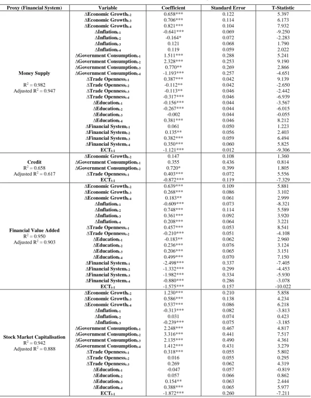
In relation to the linear growth models and the respective short-term estimates (Table 10), four conclusions should be noted. Firstly, the error correction terms are all strongly statistically significant, negative and vary from 0 to -2. This suggests that our models converge to the long-term equilibrium whenever there is any short-long-term shock or disturbance. Secondly, the lagged values of the economic growth tend to be statistically significant and positive. This confirms that Portuguese economic growth tends to be strongly persistent in line with the hypothesis of the steady-state convergence of the neoclassical growth model (Hassan et al., 2011; Breitenlechner
et al., 2015; Alexiou et al., 2018). Thirdly, the majority of variables (including those related to
the financial system) exhibits the same signs as the long-term estimates, which suggests that Portuguese economic growth is affected similarly by these variables in both the short term and the long term. Fourthly, our models present high R-squared and adjusted R-squared values, which suggests that they describe quite well the evolution of Portuguese economic growth.
_____________________________________________________________________________________ Table 10 – The short-term estimates of the linear growth models
Proxy (Financial System) Variable Coefficient Standard Error T-Statistic
Money Supply R2 = 0.982 Adjusted R2 = 0.947 ∆Economic Growtht-2 ∆Economic Growtht-3 ∆Economic Growtht-4 ∆Inflationt-1 ∆Inflationt-2 ∆Inflationt-3 ∆Inflationt-4 ∆Government Consumptiont-1 ∆Government Consumptiont-2 ∆Government Consumptiont-3 ∆Government Consumptiont-4 ∆Trade Opennesst-1 ∆Trade Opennesst-2 ∆Trade Opennesst-3 ∆Trade Opennesst-4 ∆Educationt-1 ∆Educationt-2 ∆Educationt-3 ∆Educationt-4 ∆Financial Systemt-1 ∆Financial Systemt-2 ∆Financial Systemt-3 ∆Financial Systemt-4 ECTt-1 0.658*** 0.706*** 0.821*** -0.641*** -0.164* 0.121 0.119 1.511*** 2.328*** 0.770** -1.193*** 0.387*** -0.112** -0.113** -0.317*** -0.156*** -0.267*** -0.002 0.381*** 0.061 0.135** 0.382*** 0.350*** -1.121*** 0.122 0.114 0.104 0.069 0.072 0.068 0.059 0.288 0.253 0.269 0.257 0.042 0.042 0.046 0.046 0.044 0.044 0.044 0.046 0.050 0.056 0.059 0.060 0.012 5.397 6.173 7.932 -9.250 -2.283 1.790 2.022 5.241 9.190 2.866 -4.651 9.139 -2.650 -2.442 -6.939 -3.567 -6.015 -0.055 8.212 1.223 2.403 6.494 5.825 -9.306 Credit R2 = 0.658 Adjusted R2 = 0.617 ∆Economic Growtht-2 ∆Government Consumptiont-1 ∆Government Consumptiont-2 ∆Trade Opennesst-1 ECTt-1 0.147 0.355 0.720* 0.403*** -0.872*** 0.108 0.436 0.399 0.072 0.119 1.360 0.814 1.805 5.556 -7.329
Financial Value Added
R2 = 0.950 Adjusted R2 = 0.903 ∆Economic Growtht-2 ∆Economic Growtht-3 ∆Economic Growtht-4 ∆Inflationt-1 ∆Inflationt-2 ∆Inflationt-3 ∆Inflationt-4 ∆Trade Opennesst-1 ∆Trade Opennesst-2 ∆Educationt-1 ∆Educationt-2 ∆Educationt-3 ∆Educationt-4 ∆Financial Systemt-1 ∆Financial Systemt-2 ∆Financial Systemt-3 ∆Financial Systemt-4 ECTt-1 0.639*** 0.268*** 0.183** -0.609*** 0.748*** 0.361*** 0.208*** 0.457*** -0.210*** -0.183** 0.236*** 0.206*** 0.499*** -2.498*** -1.332*** -1.982*** -0.880*** -1.575*** 0.109 0.086 0.061 0.073 0.114 0.092 0.064 0.053 0.051 0.062 0.076 0.065 0.070 0.337 0.299 0.334 0.286 0.157 5.881 3.102 2.999 -8.321 5.589 3.920 3.221 8.541 -4.108 2.960 3.124 3.151 7.150 -7.405 -4.453 -5.930 -3.078 -10.022
Stock Market Capitalisation
R2 = 0.942 Adjusted R2 = 0.888 ∆Economic Growtht-2 ∆Economic Growtht-3 ∆Economic Growtht-4 ∆Inflationt-1 ∆Inflationt-2 ∆Inflationt-3 ∆Government Consumptiont-1 ∆Government Consumptiont-2 ∆Government Consumptiont-3 ∆Government Consumptiont-4 ∆Trade Opennesst-1 ∆Trade Opennesst-2 ∆Trade Opennesst-3 ∆Educationt-1 ∆Educationt-2 ∆Educationt-3 ∆Educationt-4 ECTt-1 1.230*** 0.586*** 0.537*** -0.313*** 0.031 -0.239*** 2.248*** 3.316*** 2.135*** 1.412*** 0.318*** 0.016 0.269 -0.047 0.057 0.154** 0.388*** -1.872*** 0.210 0.138 0.086 0.082 0.074 0.075 0.467 0.441 0.490 0.431 0.055 0.055 0.062 0.057 0.066 0.063 0.065 0.260 5.858 4.234 6.218 -3.813 0.423 -3.185 4.817 7.517 4.361 3.279 5.802 0.295 4.319 -0.819 0.862 2.444 5.977 -7.211 Note: ∆ is the operator of the first differences, *** indicates statistical significance at 1% level, ** indicates statistical significance at 5% level and * indicates statistical significance at 1% level
Regarding the non-linear growth models and their long-term estimates (Table 11), results do not change dramatically in comparison with the long-term estimates of the linear growth models. Effectively, the variables that are statistically (in)significant are exactly the same, and they have the same effects on Portuguese economic growth. The most important finding pertains to the
_____________________________________________________________________________________ variables linked with the financial (banking) system by confirming the existence of a concave quadratic relationship between the financial (banking) system and Portuguese economic growth. Effectively, the linear terms of the variables of money supply, credit and financial value added are positives, the squared terms of the same variables are negatives and all of them are statistically significant. This implies a turning point of around 57.3%, 111.6% and 12.7% in the cases of money supply, credit and financial value added, respectively. The Portuguese financial (banking) system had already supplanted these thresholds by the end of the 1970s in the case of money supply, and by the mid-1990s in the cases of credit and of financial value added (Figure A1 in the Appendix), which suggests the need to decrease the importance of the financial (banking) system in the coming years to restore a supportive relationship between the financial system and economic growth in Portugal. The conclusion for stock market capitalisation is exactly the opposite. The linear term is negative, the squared term is positive and both of them are statistically significant. This indicates that the relationship between stock market capitalisation and Portuguese economic growth is indeed convex rather than concave, which is associated with a turning point of about 34.8%. Stock market capitalisation needs to surpass this threshold in the coming years in order to start to exert a positive impact on Portuguese economic growth (Figure A1 in the Appendix). This result is related with the aforementioned fact that Portugal is a ‘bank-based’ country, which seems to suggest the need to further develop the financial (stock) markets (instead of pursuing with a further development of the banking system) to reinforce the relationship between savings and investments and boost Portuguese economic growth. The structure of the Portuguese productive system, characterised essentially by small and medium corporations, should be the main obstacle to the implementation of this strategy because these corporations face more financing constraints particularly through the financial markets.
Table 11 – The long-term estimates of the non-linear growth models
Variable Money Supply Credit Financial Value
Added Stock Market Capitalisation Inflationt -0.548*** (0.120) [-4.557] -0.528*** (0.153) [-3.460] -0.572*** (0.115) [-4.989] -2.621* (0.844) [-3.104] Government Consumptiont -0.281 (0.307) [-0.917] 0.009 (0.287) [0.031] -0.763** (0.360) [-2.118] 1.014** (0.319) [3.182] Trade Opennesst 0.162** (0.071) [2.276] 0.115 (0.071) [1.621] 0.176** (0.079) [2.224] 0.863* (0.273) [3.159] Educationt -0.159** (0.060) [-2.632] -0.143* (0.075) [-1.899] -0.154** (0.061) [-2.510] -0.565** (0.151) [-3.739] Financial Systemt 0.377** (0.148) [2.544] 0.125* (0.065) [1.914] 2.542** (0.971) [2.619] -2.214* (0.828) [-2.674] Financial Systemt2 -0.329*** (0.084) [-3.934] -0.056** (0.021) [-2.616] -10.047*** (2.947) [-3.409] 3.180* (1.220) [2.606] Financial System* 57.3 111.6 12.7 34.8
Note: Standard errors in (), t-statistics in [], *** indicates statistical significance at 1% level, ** indicates statistical significance at 5% level and * indicates statistical significance at 10% level
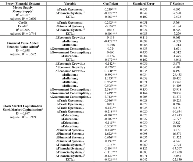
_____________________________________________________________________________________ With regard to the short-term estimates of the non-linear growth models, the conclusions are similar to those of the linear growth models. Our models are convergent and have high R-squared and adjusted R-squared values; Portuguese economic growth exhibits persistence, and the majority of variables (including variables to measure the financial system) exhibit the same signs as the long-term estimates.
Table 12 – The short-term estimates of the non-linear growth models
Proxy (Financial System) Variable Coefficient Standard Error T-Statistic
Money Supply Money Supply2 R2 = 0.707 Adjusted R2 = 0.690 ∆Trade Opennesst-1 ∆Financial Systemt-12 ECTt-1 0.249*** -0.322*** -0.769*** 0.053 0.042 0.102 4.695 -7.590 -7.522 Credit Credit2 R2 = 0.805 Adjusted R2 = 0.744 ∆Trade Opennesst-1 ∆Financial Systemt-1 ∆Financial Systemt-12 ECTt-1 0.292*** -0.168** 0.015 -0.604*** 0.051 0.077 0.024 0.083 5.764 -2.184 0.646 -7.279
Financial Value Added Financial Value Added2
R2 = 0.658 Adjusted R2 = 0.592 ∆Economic Growtht-2 ∆Inflationt-1 ∆Inflationt-2 ∆Government Consumptiont-1 ∆Government Consumptiont-2 ∆Educationt-1 ECTt-1 0.114 -0.422*** -0.018 -0.724 0.660 -0.124 -0.977*** 0.119 0.097 0.086 0.433 0.436 0.084 0.162 0.961 -4.339 -0.214 -1.671 -1.512 -1.475 -6.042
Stock Market Capitalisation Stock Market Capitalisation2
R2 = 0.997 Adjusted R2 = 0.989 ∆Economic Growtht-2 ∆Economic Growtht-3 ∆Economic Growtht-4 ∆Inflationt-1 ∆Inflationt-2 ∆Inflationt-3 ∆Inflationt-4 ∆Government Consumptiont-1 ∆Government Consumptiont-2 ∆Government Consumptiont-3 ∆Trade Opennesst-1 ∆Trade Opennesst-2 ∆Trade Opennesst-3 ∆Trade Opennesst-4 ∆Educationt-1 ∆Educationt-2 ∆Educationt-3 ∆Educationt-4 ∆Financial Systemt-1 ∆Financial Systemt-2 ∆Financial Systemt-3 ∆Financial Systemt-4 ∆Financial Systemt-12 ∆Financial Systemt-22 ∆Financial Systemt-32 ∆Financial Systemt-42 ECTt-1 0.142** 0.220** 0.300*** -0.899*** 1.133*** 0.964*** 0.505*** 2.384*** 3.419*** 2.742*** 0.546*** 0.017 0.153** -0.218*** -0.304*** -0.209*** 0.115** 0.305*** 0.150** 1.622*** 0.656*** 0.192** -0.167* -2.194*** -1.110*** -0.429*** -0.926*** 0.039 0.045 0.035 0.034 0.058 0.071 0.035 0.150 0.164 0.205 0.028 0.029 0.028 0.020 0.023 0.027 0.030 0.029 0.046 0.098 0.057 0.045 0.060 0.125 0.083 0.071 0.042 3.673 4.884 8.497 -26.453 19.420 13.542 14.408 15.918 20.838 13.372 19.224 0.594 5.418 -10.634 -13.413 -7.777 3.822 10.500 3.279 16.579 11.522 4.249 -2.794 -17.507 -13.428 -6.053 -22.130
Note: ∆ is the operator of the first differences, *** indicates statistical significance at 1% level, ** indicates statistical
significance at 5% level and * indicates statistical significance at 1% level
To summarise, we find a disruptive (linear) relationship between the financial (banking) system and Portuguese economic growth, which corroborates that the hypothesis on the finance-growth nexus has lost relevance in times of financialisation. We also find a quadratic (non-linear) relationship between the financial (banking) system and Portuguese economic growth, suggesting the need to revert their importance in the coming years to promote more economic growth in Portugal. The conclusions for the variable of stock market capitalisation are exactly the opposite. The linear relationship is positive and the non-linear relationship is convex, suggesting the need to further develop the financial (stock) markets in order to sustain more economic growth in Portugal.
_____________________________________________________________________________________
7. CONCLUSION
This study performed a time series econometric analysis in order to assess the relationship between the financial system and the economic growth in Portugal over 40 years, from 1977 to 2016.
During that time, and particularly after the mid-1980s, the Portuguese financial system suffered a strong transformation, which occurred due to the widespread privatisations, liberalisations and deregulations of financial activities in order to fulfil the European rules due to the integration process, which began in 1986 with the adhesion of Portugal into the European Economic Community (Barradas et al., 2018). As a result, the financial system gained huge importance (i.e. the so-called financialisation), which did not translate into a sustained path of a strong economic growth in Portugal. This casts doubts on the hypothesis of the finance-growth nexus, which has been already corroborated by other empirical works that have found a weakening or even a reversal in the relationship between the financial system and economic growth for a significant variety of countries and/or time periods (Rioja and Valev, 2004a and 2004b; Aghion et al., 2005; Kose et al., 2006; Prasad et al., 2007; Rousseau and Wachtel, 2011, Cecchetti and Kharroubi, 2012; Barajas et al., 2013; Dabla-Norris and Srivisal, 2013; Beck et al., 2014; Breintenlechner et al., 2015; Ehigiamusoe and Lean, 2018; Alexiou et al., 2018).
We estimated a linear growth model and a non-linear growth model by implementing the ARDL estimator in EViews software, taking into account that we have a mixture of variables that are integrated of order zero and variables that are integrated of order one. We used four proxies for the financial system (money supply, credit, financial value added and stock market capitalisation) in order to reflect in a more complete way the role of financial system, namely, by encompassing proxies related to the banking system (the first three) and a proxy related to financial markets (the fourth) that simultaneously assess its size, depth and efficiency (Beck et
al., 2014; Breitenlechner et al., 2015). Inflation, government consumption, trade openness and
education are used as control variables in our estimates, following other empirical studies of the finance-growth nexus (Rioja and Valev, 2003; Rousseau and Wachtel, 2011; Hassan et al., 2011; Beck et al., 2014; Jedidia et al., 2014; Breitenlechner et al., 2015; Durusu-Ciftci et al., 2017; Ehigiamusoe and Lean, 2018; Alexiou et al., 2018).
Our results confirm the results of the majority of these empirical works both in the long term and in the short term. Inflation exerts a negative effect on Portuguese economic growth, whilst trade openness exerts a positive effect. Portuguese economic growth is strongly persistent. Our results are not in line with the hypothesis of the finance-growth nexus, particularly with regard to proxies more linked with the banking system. On the one hand and with regards to the linear growth model, our results show that the financial (banking) system negatively influences
_____________________________________________________________________________________ Portuguese economic growth. Regarding the non-linear growth model, our results confirm the existence of a concave quadratic relationship between money supply, credit and financial value added and Portuguese economic growth. On the other hand, our results show a supportive (linear) relationship and a convex quadratic relationship between stock market capitalisation and Portuguese economic growth.
Our results therefore provide very important insights for policy makers in order to support higher economic growth in the coming years. Portuguese policy makers should adopt measures in order to contain inflation (although this corresponds effectively to a mission of the European Central Bank) and to promote a higher degree of openness of the Portuguese economy. Additionally, they should adopt measures to invert the growth of the financial (banking) system because Portugal has already supplanted the threshold values of money supply, credit and financial value added from which they favour a higher economic growth. A higher development of the financial (stock) markets could be desirable, given that they are underdeveloped in Portugal and they still represent less than the respective threshold from which they boost economic growth.
_____________________________________________________________________________________
8. REFERENCES
AGHION, P.; Howitt, P.; and Mayer-Foulkes, D. 2005. ‘The Effect of Financial Development on Convergence: Theory and Evidence’. Quarterly Journal of Economics, 120 (1): 173-222. ALEXIOU, C.; and Nellis, J. 2013. ‘Challenging the Raison d'etre of Internal Devaluation in the Context of the Greek Economy’. Panoeconomicus, 60 (6): 813–836.
ALEXIOU, C.; Vogiazas, S.; and Nellis, J. 2018. ‘Reassessing the relationship between the financial sector and economic growth: Dynamic panel evidence’. International Journal of Finance & Economics. 23 (2): 155-173.
ANG, J. B. 2008. ‘A Survey of Recent Developments in the Literature of Finance and Growth’. Journal of Economic Surveys. 22 (3): 536-576.
ARESTIS, P.; Chortareas, G.; and Magkonis, G. 2015. ‘The Financial Development and Growth Nexus: A Meta-Analysis’. Journal of Economic Surveys. 29 (3): 549-565.
BARAJAS, A.; Chami, R.; and Yousefi, S. R. 2013. ‘The Finance and Growth Nexus Re-Examined: Do All Countries Benefit Equally?’. IMF Working Paper 13/130.
BARRADAS, R. 2016. ‘Evolution of the Financial Sector – Three Different Stages: Repression, Development and Financialisation’. In Advances in Applied Business Research: the L.A.B.S. Initiative. Gomes, O. and Martins, H. F. (ed.): New York: Nova Science Publishers.
BARRADAS, R. 2017. ‘Financialisation and Real Investment in the European Union: Beneficial or Prejudicial Effects?’. Review of Political Economy. 29 (3): 376-413.
BARRADAS, R. 2019. ‘Financialization and Neoliberalism and the Fall in the Labor Share: A Panel Data Econometric Analysis for the European Union Countries. Review of Radical Political Economics. 51 (3): 383-417.
BARRADAS, R.; and Lagoa, S. 2017a. ‘Functional Income Distribution in Portugal: The Role of Financialisation and Other Related Determinants’. Society and Economy, 39 (2): 183-212.
BARRADAS, R.; and Lagoa, S. 2017b. ‘Financialisation and Portuguese real investment: A supportive or disruptive relationship?’. Journal of Post Keynesian Economics. 40 (3): 413-439.