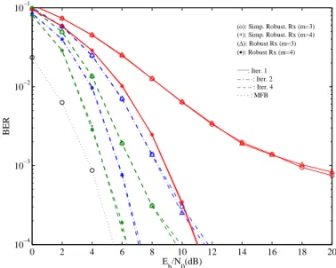
Robust receivers for base station cooperation systems

HbA1c, observação dos pés, ensinos realizados e metas estabelecidas. Como principal conclusão obtivemos que existem poucas diferenças entre as recomendações avaliadas da NOC e

Deste modo, para os críticos que pensam des- de o Norte, a bioética principialista é passível de críticas apenas enquanto uma pretensa teoria, isto é, centram a discussão

Barroso, na interpretação de John Coltrane: a utilização da composição como veículo para a improvisação no jazz

Peça de mão de alta rotação pneumática com sistema Push Button (botão para remoção de broca), podendo apresentar passagem dupla de ar e acoplamento para engate rápido

do Homem Económico Organizacional Organizacional Social Administrativo Funcional Complexo Sistema de Incentivos Materiais e salariais Materiais e salariais Mistos: materiais e

Comparing costs of two offered scenarios for this production line, it is shown that the second scenario has a lower cost and its better for the system to produce completed MTS

As redes sociais são tecnologias de grande valia para a manutenção da saúde das pessoas e podem propiciar informações e trocas valiosas, auxiliando no

Outros estudos complementares indicam que como os idosos com DA possuem menor reserva de atenção, se comparados com indivíduos com envelhecimento normal, e