❊♥s❛✐♦s ❊❝♦♥ô♠✐❝♦s
❊s❝♦❧❛ ❞❡
Pós✲●r❛❞✉❛çã♦
❡♠ ❊❝♦♥♦♠✐❛
❞❛ ❋✉♥❞❛çã♦
●❡t✉❧✐♦ ❱❛r❣❛s
◆◦ ✸✻✾ ■❙❙◆ ✵✶✵✹✲✽✾✶✵
❆r❡ ❖♥❡✲❙✐❞❡❞ ❙✱s ❘✉❧❡s ❯s❡❢✉❧ Pr♦①✐❡s ❋♦r
❖♣t✐♠❛❧ Pr✐❝✐♥❣ ❘✉❧❡s❄
▼❛r❝♦ ❆♥tô♥✐♦ ❈❡s❛r ❇♦♥♦♠♦
❖s ❛rt✐❣♦s ♣✉❜❧✐❝❛❞♦s sã♦ ❞❡ ✐♥t❡✐r❛ r❡s♣♦♥s❛❜✐❧✐❞❛❞❡ ❞❡ s❡✉s ❛✉t♦r❡s✳ ❆s
♦♣✐♥✐õ❡s ♥❡❧❡s ❡♠✐t✐❞❛s ♥ã♦ ❡①♣r✐♠❡♠✱ ♥❡❝❡ss❛r✐❛♠❡♥t❡✱ ♦ ♣♦♥t♦ ❞❡ ✈✐st❛ ❞❛
❋✉♥❞❛çã♦ ●❡t✉❧✐♦ ❱❛r❣❛s✳
❊❙❈❖▲❆ ❉❊ PÓ❙✲●❘❆❉❯❆➬➹❖ ❊▼ ❊❈❖◆❖▼■❆ ❉✐r❡t♦r ●❡r❛❧✿ ❘❡♥❛t♦ ❋r❛❣❡❧❧✐ ❈❛r❞♦s♦
❉✐r❡t♦r ❞❡ ❊♥s✐♥♦✿ ▲✉✐s ❍❡♥r✐q✉❡ ❇❡rt♦❧✐♥♦ ❇r❛✐❞♦ ❉✐r❡t♦r ❞❡ P❡sq✉✐s❛✿ ❏♦ã♦ ❱✐❝t♦r ■ss❧❡r
❉✐r❡t♦r ❞❡ P✉❜❧✐❝❛çõ❡s ❈✐❡♥tí✜❝❛s✿ ❘✐❝❛r❞♦ ❞❡ ❖❧✐✈❡✐r❛ ❈❛✈❛❧❝❛♥t✐
❆♥tô♥✐♦ ❈❡s❛r ❇♦♥♦♠♦✱ ▼❛r❝♦
❆r❡ ❖♥❡✲❙✐❞❡❞ ❙✱s ❘✉❧❡s ❯s❡❢✉❧ Pr♦①✐❡s ❋♦r ❖♣t✐♠❛❧ Pr✐❝✐♥❣ ❘✉❧❡s❄✴ ▼❛r❝♦ ❆♥tô♥✐♦ ❈❡s❛r ❇♦♥♦♠♦ ✕ ❘✐♦ ❞❡ ❏❛♥❡✐r♦ ✿ ❋●❱✱❊P●❊✱ ✷✵✶✵
✭❊♥s❛✐♦s ❊❝♦♥ô♠✐❝♦s❀ ✸✻✾✮
■♥❝❧✉✐ ❜✐❜❧✐♦❣r❛❢✐❛✳
ARE ONE-SIDED S,s RULES
USEFUL PROXIES FOR OPTIMAL PRICING RULES?1
MARCO BONOMO
GRADUATE SCHOOL OF ECONOMICS
GETULIO VARGAS FOUNDATION
Praia de Botafogo 190 sala 1125, Rio de Janeiro, RJ 22253-900, Brasil
e-mail: [email protected]
Abstract
This article is motivated by the prominence of one-sided S,s rules in the literature and by the unrealistic strict
conditions necessary for their optimality. It aims to assess whether one-sided pricing rules could be an
adequate individual rule for macroeconomic models, despite its suboptimality. It aims to answer two questions.
First, since agents are not fully rational, is it plausible that they use such a non-optimal rule? Second, even if the
agents adopt optimal rules, is the economist committing a serious mistake by assuming that agents use one-sided Ss
rules? Using parameters based on real economy data, we found that since the additional cost involved in
adopting the simpler rule is relatively small, it is plausible that one-sided rules are used in practice. We also
found that suboptimal one-sided rules and optimal two-sided rules are in practice similar, since one of the
bounds is not reached very often. We concluded that the macroeconomic effects when one-sided rules are
suboptimal are similar to the results obtained under two-sided optimal rules, when they are close to each other.
However, this is true only when one-sided rules are used in the context where they are not optimal.
1
1. INTRODUCTION
Some recent literature in macroeconomics was dedicated to study the macroeconomic
implications of individuals adopting one-sided Ss rules (e.g., Blinder (1981), Caplin (1985), Caplin
and Spulber (1987), Caballero and Engel (1991,1993), Foote (1998), Tsiddon (1991)).
The growing interest in one-sided Ss rules reflects in part the attention shift from
time-dependent to state-time-dependent policies. State-time-dependent policies have well-known microeconomic
foundations23 and their macroeconomic implications had been little explored until a few years ago.
The focus of the state-dependent literature on one-sided Ss rules can be justified on the grounds of
the latter being a reasonable description of reality. This is especially true in the context of pricing
policy. Other reasons for the emphasis are the tractability and the appealing results obtained with
this simple rule. One example of the latter is the money neutrality result of Caplin and Spulber
(1987)4.
Given the prominence of the one-sided Ss pricing policies in the literature, it is time to
devote some effort to the evaluation of their plausibility. This paper intends to reduce this gap5. It
2Sheshinski and Weiss (1977,1983), Caplin and Sheshinski (1987) and Bénabou (1988) derive one-sided Ss pricing rules as optimal policies in different settings.
3
A Taylor type of time-dependent rule requires a non-natural assumption about the adjustment costs: that the cost of change price cannot be dissociated from the cost of observe the level of the frictionless optimal process (see Bonomo and Carvalho 1999).
4
This is a particular instance of a more general property, which is obtained when the frictionless optimal level of the control variable is monotonic: if the distribution of the individual deviations of the controlled variable from the frictionless optimal level is uniform, the average deviation is always constant (see, for example Caballero and Engel (1991) for that and other properties).
5
This work is related to Tsiddon (1993), but its purpose is different. There a suboptimal one-sided rule is calculated only because it has a closed-form solution when there is no time discounting. It is assumed that it is close enough to the optimal two-sided rule to yield a good analytical
does it under two aspects6. First, since agents are not fully rational, it investigates whether it is
plausible that they actually use such a non-optimal rule. Second, assuming that agents adopt optimal
rules, it evaluates whether the economist is committing a serious mistake by assuming that agents
use one-sided Ss rules. In the remaining part of this introduction, we explain the approach we used
to answer to appraise those issues.
A state-dependent rule is a natural outcome when there is a deterministic and non-convex
cost of adjustment.7 In this context, we use the term frictionless optimal level to denote the optimal
level of the control variable in the absence of adjustment costs. Since optimal adjustments are
infrequent, usually the level of the control variable differs from the frictionless optimal level. The
discrepancy between the level of the control variable and its frictionless optimal level is often the
state-variable in this kind of problem8. A two-sided rule9 entails both an upper and a lower bound to
this discrepancy, while a one-sided rule limits the discrepancy in only one direction.
The issue in question concerns the conditions for the optimality of the one-sided Ss rule. It
arises because optimality of one-sided rules requires a strict hypothesis for the stochastic process of
the frictionless optimal level of the control variable, which in some applications is hardly satisfied10:
that its level is monotonic with respect to time. When the control variable is the price charged by an
agent, this means that the frictionless optimal level for an individual price never decreases. If the
frictionless optimal level of the control variable follows a process that has a trend, but it is not
6
Another type of evaluation is provided by Tommasi (1996), which evaluates the performance of one-sided S,s rules as a forecast rule. His findings are that S,s rules have a better relative performance for high inflation, but perform poorly at hyperinflation.
7
Other recent work consider stochastic adjustment costs, generating individual stochastic rules (e.g. Caballero and Engel 1999,and Dotsey, King and Wolman 1999).
8
In some few articles the adjustment problem has more than one state-variable (e.g. Bonomo and Garcia 1998, and Conlon and Liu 1997).
9
Caplin and Leahy (1991,1997), Caballero and Engel (1992), and Almeida and Bonomo (1999) are examples of macroeconomic models based on two-sided pricing rules.
10
monotonic with respect to time, the optimal policy is a two-sided rule.
If the drift is large, when compared to the variance of shocks, it is possible that one of the
bounds will be very little active. For example, when average inflation is very high, when compared
to the variance, the discrepancy between the individual price and its frictionless level will have a
negative drift. Then, the probability that the deviation process increases by a given amount in a
certain interval of time also will be small. Moreover, the upper bound of the band is likely to be
large. Thus, the probability that the deviation process reaches the upper barrier, in a given interval of
time, tends to be very small. Therefore, one may argue that, in practice, it is as if the policy were
one-sided.
One may also argue that in the case above, the loss involved in adopting a simpler
suboptimal one-sided Ss rule is very small, and consequently the agents are likely to adopt such
rules in that context. This could be justified by near rationality or, alternatively, by the existence of a
small extra cost involved in using a more complex rule.
Our objective is to assess the validity of those arguments in the light of plausible parameter
values for the frictionless optimal-price process. Our formulation of the control problem is based on
Dixit (1991b), which developed an analytically simpler framework for the optimal control of
Brownian Motions.
Our simulations of both the optimal two-sided and the suboptimal one-sided pricing policies,
with parameters for the frictionless optimal price process based on real economy data, show that
these policies are close to one another. Furthermore, the additional cost of adopting a suboptimal
one-sided rule is small, making the adoption of the simpler suboptimal one-sided rule plausible.
Because of their closeness, optimal two-sided and suboptimal one-sided rules have similar
macroeconomic consequences. However, it is important to notice that optimal and suboptimal
entail different macroeconomic effects. Suboptimal one-sided rules do not produce the same kind of
neutrality results generated by optimal one-sided rules. Even when a suboptimal one-sided rule is
close to optimal, there might be small negative shocks that have contractionary effects on output.
Those negative shocks have large effect, as compared to their magnitude. On the other hand, in this
context, positive shocks have relatively small effects. Thus, suboptimal one-sided rules not only are
realistic microeconomic rules but also produce realistic macroeconomic effects, generating
substantial price rigidity asymmetry, as found in the data11.
We proceed as follows. Section 2 characterizes the solution for the optimal policy, which is
an asymmetric two-sided rule, when the frictionless optimal value for the control variable follows a
Brownian motion with drift. It also solves for the best one-sided rule. Section 3 derives the expected
time until the upper (lower) bound is reached for the first time. Section 4 makes a numerical
assessment of how close the optimal two-sided and the best one-sided rules are to each other
according to two approaches. First, it calculates the expected time until the upper bound is attained,
which is an inverse measure of how often the upper bound is reached. Second, it evaluates the
additional cost incurred when the suboptimal one-sided Ss rule is adopted, instead of the optimal
one. It then analyses how sensitive the results are to changes in the parameter values. Finally, we fix
time-discount and menu costs parameters, and compare optimal two-sided and suboptimal
one-sided rules when stochastic processes for the frictionless optimal price are calibrated to replicate the
time pattern of the nominal aggregate demand in selected international experiences. Section 5
speculates about the possible macroeconomic implications of the results obtained. The last section
concludes.
2. OPTIMAL TWO-SIDED AND SUBOPTIMAL ONE-SIDED RULES
In this section, we derive both the optimal pricing policy - which is an asymmetric two-sided
rule - and the best one-sided policy.
The following are the basic assumptions related to the individual agent's decision problem.
The optimal price of the firm follows a geometric Brownian motion. So the (unconstrained) optimal
value for the logarithm of the price charged by the firm, p*, will follow a Brownian motion, that is:
where {ws} is a Wiener process. However there is a lump-sum adjustment cost, k, which is paid
every time the price is changed, and there is a quadratic flow cost for being away from the optimal
price. We assume that a deviation of the (log of the) control variable p from the unconstrained
optimal level p* brings an instantaneous flow cost h(pt-pt*)2dt. Time is discounted at the continuous
rate, ρ, which is constant through time.
This is what is called a problem of impulse control. In this type of control problem, the
adjustment cost function makes optimal infrequent jumps of the control variable, instead of
continuous small adjustments. An impulse control problem, similar to this, was first solved by
Harrison, Selke and Taylor (1983).12 Making use of a simpler framework, Dixit (1991b) presents
the solution for classes of cost functions, which include the ones used here. We follow his
approach.
We define the cost function as the loss of value imposed by the existence of adjustment
costs if the agent acts in an optimal way. Therefore, if there were no adjustment costs the agent
12
Following a different approach, Tsiddon (1993) characterizes the optimal policy for the
dw s + mdt =
dp t
*
would set the control variable always equal to the frictionless optimal value and the cost function
would be identically to zero.
Formally, the cost function can be written as:
where
That is, the problem can be stated in terms of controlling the difference between the log of
the original control variable and the log of its frictionless optimal value. It is clear that if no control is
exerted, x will follow a Brownian motion with drift η=-m and variance σ=s. The problem consists
in finding the optimal value for three numbers, a<c<b, such that if either a or b is reached, control is
exercised and x is reset to c.13
If a<x<b, no jump takes place in a small interval of time dt. Then, the cost function at time
zero can be written as the flow cost at the next infinitesimal interval of time plus the expectation of
the cost function at the end of this interval:
Since a<x<b, x is following a Brownian motion at the next infinitesimal time. So, we can apply Ito's
Lemma to dC(xt) and take expectations conditioned on the knowledge of xt to arrive at an
expression for the expectation term in the equation above. Substituting it into (4) and then
rearranging it, we obtain the following differential equation for C:
undiscounted problem.
13 That the optimal resetting from both the upper and lower barrier is made to the same place is a feature of the lump-sum adjustment costs.
[
hx e dt+ ke |x =x]
minE =
C(x) t 0
-i t -2 t 0 i ρ ρ ∑
∫∞ (2)
p -p =
xt t *t
x] = x | ) dx + E[C(x e + dt hx =
C(x) 2 -ρdt t t
(4) 0 = hx + C(x) -(x) C + (x) C 2
1 2 2
ρ η
which implies that C has the following general form:
where:
The first two terms in equation (6) are the solutions for the homogeneous equation. The
remaining ones constitute a particular solution, namely, the expected discounted cost of the
uncontrolled process14. The cost functions of the uncontrolled process and of any process controlled
by barriers follow the same differential equation (5)15. The control adds other restrictions that
determine the values of the constants A and B in the cost function (6).
A. The two-sided optimal rule
The Value Matching Conditions (VMC) state that the cost at a (b) should be equal to the
cost at c plus what is paid for moving from a (b) to c, that is k16. So, V(a)= V(c)+k and
14This can be found by integrating the expression of the expected present value of the cost of the uncontrolled process.
15This is a feature of the differential approach where the probability of reaching a barrier at the next infinitesimal time, from a point inside the band, is also infinitesimal.
16The VMC introduce mathematically the control into the solution. For chosen values a,c,b the VMC allow us to determine A and B, in order to find the cost function generated by this policy. The VMC are just consistency requirements for the expected present cost of a given policy.
ρ η ρ σ ρ η ρ β α 3 2 2 2 2 2 x
x +hx +2 h x +h +2h
V(b)=V(c)+k . Using (6) we have the following equations:
The Smooth Pasting Conditions (SPC) tell us that the derivative of the value function at the
points a,c and b should be equal to the derivative of the adjustment cost17. So, V'(a)=V'(c)=V'(b)=0
. Together with the VMC (8) and (9), they allow us to find the optimal values for a,c and b. Using
(6) we get the following SPC:
0 = 2 + c 2 h + Be + Ae 2 c c ρ η ρ β
α α β (12)
The VMC and SPC equations , (8,9,10,11,12), constitute a non-linear system of five
17The SPC are optimality conditions for policy parameters. For a simple derivation of the SPC, see Dixit (1991b).
k = c) -(a 2 + ) c -a ( 1 h + ) e -e B( + ) e -e
A( a c a c 2 2 2
ρ η ρ β β α α (8) k = c) -(b 2 + ) c -b ( 1 h + ) e -e B( + ) e -e
A( b c b c 2 2 2
ρ η ρ β β α α (9) 0 = 2 + a 2 h + Be + Ae 2 a a ρ η ρ β
α α β (10)
0 = 2 + b 2 h + Be + Ae 2 b b ρ η ρ β
equations and five unknowns, which can only be solved numerically18.
B. The one-sided suboptimal rule
Now we impose the form of the policy to be a one-sided rule, and determine the best policy
of its form.
First, observe that the cost function for the one-sided rule, for the same reasons given above
for the two-sided rule, should satisfy the differential equation given by (5). Thus, it has a general
solution given by (6), where α and β are the roots of the characteristic equation of (5) and have
opposite signs: α<0, β>0. The form of our suboptimal one-sided rule will depend on the sign of the
drift. In order to keep the most useful barrier, we will drop the upper barrier, if the drift of the
uncontrolled process is negative, and will drop the lower one, if it is positive.
We will assume the drift is negative. Therefore, we will not have any upper barrier. The
process is allowed to take any arbitrary large value. Starting from a very large value, the probability
of hitting the lower barrier within a reasonable amount of time is very small, and, consequently, the
cost function should be close to the cost function of the uncontrolled process. When x is very large,
the first term of (6) is close to zero (α is negative), but the second also becomes very large, unless B
is zero. For the cost function to be approximated by the four last terms in (6) (the cost function of
the uncontrolled process) when x becomes very large, it is necessary that B=0. Hence, our general
equation for the cost function, when the control rule is a one-sided resetting policy is:
Equation (13) together with the VMC linking b and c determine the cost function
for an arbitrarily chosen one-sided policy (b,c). Using (13), the VMC becomes:
18When the uncontrolled process has no drift, the problem becomes much simpler with a=-b and
0 = 2h + h + x 2h + x h + e
A 3
2
2 2
2 2
x
ρ η ρ
σ ρ
η ρ
Again, the SPC give optimality conditions for the choice of the parameters, a and c. The
SPC are:
Equations (14), (15) and (16) determine the cost function and the suboptimal policy
parameters a and c. As before, it is still not possible to find explicit solutions, forcing us to use
numerical techniques.
The increase in cost of adopting the suboptimal one-sided rule, as a fraction of the cost
when the optimal two-sided rule is adopted (r), can now be easily calculated. Let the expected cost
starting from x using the optimal rule, C2(x), be given by the cost function (6) when the constants A
and B are calculated solving the equations (8) to (12). Let the expected cost starting from x when
the suboptimal one-sided rule is used, C1(x), be given by (13) when A is calculated solving the
equations (14) to (16). Then, the relative increase in cost starting at x is given by:
c=0. Dixit (1991a) finds an approximated analytical solution for this case. k = c) -(a 2 + ) c -a ( 1 h + ) e -e
A( a c 2 2 2
ρ η ρ α α (14) 0 = 2 + a 2 h + Ae 2 a ρ η ρ
α α (15)
0 = 2 + c 2 h + Ae 2 c ρ η ρ
α α (16)
3. THE EXPECTED TIME OF HITTING A SPECIFIC BARRIER FOR THE FIRST
TIME
In order to assess how far the two-sided policy is from a one-sided one, it would be useful
to have an idea of the time spent before an specific barrier (the one that is not hit very often) is hit,
starting from a position x. Notice that calculating the distribution of the time until hitting a specific
barrier for the first time, is much more involving than finding the distribution of the time until hitting
any barrier for the first time. The latter depends only on the probability law of the Brownian motion,
whereas the former has to take into account that a possible resetting in the other barrier may occur,
before the specific barrier is hit. Furthermore, the distribution that would interest us does not have a
closed form solution. Nevertheless, following a relatively simple approach, we can find an explicit
formula for the expected time until reaching a specific barrier starting from x. So, we chose to do it
instead.
The approach we use is similar to the one employed to calculate the value function
corresponding to a specific policy (a,c,b).19Let Tb be the time the controlled process X hits the
barrier b for the first time. We define θb(x) = E x
Tb , that is, θb(x) is the expected time, starting at x,
until the process X hits the barrier b for the first time. So, θb satisfies the following Bellman
equation:
Applying Ito's Lemma to dθ(xt) and taking expectations conditioned on the knowledge of xt , one
can arrive at an expression for the expectation term in the equation above. After substituting it into
(18) we obtain the following differential equation for θ:
19This is an extension of Karlin and Taylor (1981,pp192-3).
x] = x | ) dx + (x E[ + dt =
(x) b t t
b θ
θ (18)
0 = 1 + (x) + (x) 2
1σ2θ′′ ηθ′
The general solution to this differential equation is:
Now, consistency conditions, analogous to VMC, allow us to find the constants A and B
corresponding to the policy parameters (a,c,b).20
The conditions are:
Equations (21) have obvious interpretations. The expected time until hitting b for the first time
starting from b is 0. The expected time of hitting b from a has to be equal to the expected time of
hitting b from c, since when the process is in a, it is instantaneously reset to c.
Using conditions (21) to determine the constants A and B in equation (20), we arrive at the
following formula for θb:
The formula of θa can be easily found by symmetry:
4. NUMERICAL ANALYSIS
20Observe that in equation (19) the policy parameters do not appear explicitly.
B + x -Ae = (x) -2 x
To do numerical exercises with parameters based on real data, it is necessary to have an
equation that relates the optimal individual price with the aggregate and idiosyncratic shocks. We
assume that the (log of) the optimal individual price, pi *
, is given by21:
where y is the (log) of nominal aggregate demand and ei is an idiosyncratic component. In the
absence of control, a change in the nominal aggregate demand will have an effect on the difference
between the actual price and the optimal frictionless price of the same magnitude and opposite
direction. We assume that the (log of) nominal aggregate demand follows a Brownian motion. We
choose the drift and diffusion parameters of the deviation process by equating them to the
symmetric of the mean and the standard deviation of the changes in the (log of) nominal aggregate
demand observations, respectively. As for the idiosyncratic component, we assume it follows a
Brownian motion without drift, independent of the stochastic process followed by the nominal
aggregate demand. So,
where s=σy+σe.
This section assesses how different optimal two-sided Ss rules are from suboptimal
one-sided Ss rules. We use two notions for that. The first is related to the observational difference of the
processes controlled by the two rules. Does the trajectory of the control variable under the optimal
two-sided rule look as the one controlled by a suboptimal one-sided Ss rule? If the upper bound is
21This formulation implies that a 1% shock in nominal aggregate demand has a 1% impact in the frictionless optimal price. Since we fix the reference period for the flows in one year, this is not without loss of generality.
e + y =
p i
*
i (24)
sdw + mdt = p
dw = e
dw + mdt = y
i *
i
ei e i
1 y
σ σ
very rarely achieved the two-sided Ss rule, in practice, looks like a one-sided one, and has similar
macroeconomic implications22. The expected time until reaching the upper bound provides us with
useful information for this assessment. We chose to evaluate the expected time of reaching the
upper bound at 0, when the actual price is equal to the optimal one, θb(0)
23
. The expected time until
reaching the most often reached bound - the lower bond a- is also calculated to give us a notion of
how often a price adjustment occurs in this economy.
The second is related to the likelihood that an economic unit adopts the suboptimal
one-sided rule instead of the optimal two-one-sided one. We evaluate how costly it is to adopt the
suboptimal one-sided rule instead of the optimal two-sided one. For this purpose, we evaluate
r(0)24, which gives the increase in cost of adopting the suboptimal one-sided rule as a fraction of the
cost when the optimal two-sided rule is adopted, evaluated at x=0.
We proceed in two steps. First, we perform some simulations in order to get some
qualitative assessment on how changes in parameter values affect the comparison. This helps us
build intuition for the comparison based on numbers for actual economies, rendered in the second
step.
22As explained in section 5 below, it has similar macroeconomic implications to the ones of one-sided rules, when those rules are used in the same environment – an environment where the one-sided rules are not optimal.
23In Bonomo (1992) the expected time until reaching each barrier starting from c - the point to which the difference between actual and optimal prices returns after an adjustment - is also reported.
A. Evaluating the parameter effects
In Table 1, we vary one parameter at a time to appraise the influence of that parameter on
the comparison25. The first column gives results for the base values we chose for the parameters:
η=-0.1, σ=0.1, ρ=2.5% and k=0.01 (since k and h enter the solution only through k/h, we
normalize h to one)26,27. Every time the actual price becomes 14% lower (a=-14%) or 20%
(b=20%) higher than the optimal price, it is reset to a value 5% (c=5%) higher than the optimal one.
Observe that the price is not reset to the value of the optimal price itself, because the optimal price
has a tendency to increase. So, anticipation of this tendency, and knowledge that the price should
remain fixed for a while because of the menu costs, lead the agent to reset the price to a level a
higher than the frictionless optimal one. Since the magnitudes of the upper and lower edges of the
band are not so different, and there is a sizeable downward drift, the lower edge is reached much
more often than the upper edge. This is reflected in the much higher value for the expected time
until reaching the upper extreme than the expected time until reaching the lower extreme. Starting at
the resetting price (c), the expected time until reaching the lower barrier for the first time is 1.82
years, while doing the same computation for the upper barrier gives 30.42 years. When we use the
best one-sided policy, instead of the two-sided policy, A, a and c are very similar to what we had
before. The absence of an upper barrier makes it safer to reset to a price a little bit lower than
25We keep the discount rate constant at ρ=0.025 since it does not affect substantially the optimal or the suboptimal policies. In Bonomo (1992) we report the result of an increase in ρ to 0.10 while keeping the other parameters constant.
26The value of k is chosen to give reasonable predictions for the frequency of price adjustments when the model is calibrated to the U.S. The value chosen for ρ is standard in the literature, and alternative reasonable values produce very similar results.
before, so c is slightly smaller now. The percentage increase in cost caused by the use of the
suboptimal one-sided rule is calculated in 6.6%, when we use base values for the parameters.
In the second column, we increase k, the ratio between the menu cost and the flow cost,
from 0.01 to 0.05. The increase in k affects dramatically the results turning the optimal policy much
closer to the suboptimal one. The band becomes much wider, increasing the expected time until
reaching the lower and the upper barrier. The effect on the expected time until reaching the upper
barrier is striking. It increases from 31.16 to 216.06 years. So, the upper bound becomes somewhat
superfluous and the adoption of the one-sided rule becomes almost costless (λ(0) is 0.9 %).
It is intuitive that when the absolute value of the drift increases, ceteris paribus, the loss
involved in adopting the suboptimal one-sided rule decreases. In addition, since the stochastic
component is symmetric, when the variance increases, ceteris paribus, the loss involved in adopting
the one-sided rule increases. Therefore, we pursue the more obscure question of what happens
when both the variance and the drift vary in the same direction. In the third column, we double both
the drift and the standard deviation. A higher variance makes the expected time until reaching a
barrier for the first time, substantially smaller. So, the size of the band widens as a response, but the
expected time continues to be smaller than before. We see that the effect of the increase in the
variance dominates the effect of the higher drift since the additional cost of imposing a one-sided
rule increased from 6.6% to 24.8%. In the fourth column, we double the drift and variance. Now
the effect of the drift is prevalent (r(0) is reduced from 6.6% to 3.1%), although the resulting effect
is of smaller magnitude than the one we had before. Since the additional cost of adopting a
suboptimal one-sided pricing rule is not a function alone of m/s2, it becomes interesting to
investigate what is the shape of the relation between m and s2 that keeps r constant.
Figure 1 depicts the relation between m and s2 for r equal to 0.01, 0.05 and 0.10. The
makes the optimal policy closer to the best one-sided rule. We see that the relation is not a straight
line: the increase in m necessary to compensate a given increase in s2 in order to keep r constant, is
decreasing in s2. Hence, an increase in s2 requires a less than proportional increase in m to maintain r
constant. In Figure 2, we explore the influence of k in the shape of the iso-r. We see that the lower
is k the higher the concavity of the curve. Figure 3 illustrates that if we substitute s for s2 in the
ordinate, the curve becomes convex. Thus, in general, to keep r constant when m is increased, it is
necessary to increase the variance more than proportionally, but by less than the addition that would
cause a proportional increase in the standard deviation.
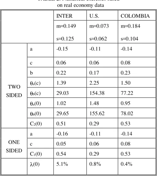
B. Comparison of the rules based on real economies
In Table 2, we present results with parameter values based on real economy data. We chose
one low inflation economy (U.S.), one high inflation economy (Colombia), and an average of 43
countries (Inter)28. We base our values on Ball, Mankiw and Romer (1988) data. For each process,
we calibrate the drift to the respective average increase in the log of the nominal aggregate demand.
As for the diffusion coefficient, an allowance for the standard deviation of idiosyncratic shocks is
added to the standard devialtion of the log of the nominal aggregate demand. For the U.S., we
assume that the standard deviation of the idiosyncratic shocks is 5.3% (an assumption that exceeds
the 3% used in Ball, Mankiw and Romer (1988)). For the set of countries, we use 8.8%, and for
Colombia, 8.2%. The implicit assumption is the standard deviation of the idiosyncratic shocks
increase with inflation, but not dramatically. Observe that, when we use k=0.01, the model produces
reasonable predictions for the U.S. economy. The expected time until an upward price adjustment
starting from c (the value at which the price is reset) is a good approximation for the time between
adjustments, since a downward adjustment does not happen often. So, according to the model, the
elapsed time between adjustments should be a little bit more than two years (since θa(c)=2.25),
which is consistent with the microeconomic evidence29. However, the expected time until a
downward revision, seems to be very big, 154 years. As a contrast, using Colombia data, the
number obtained for the expected time until adjustment is lower, 77.22 years, despite the larger
inflation. This may suggest that the one-sided Ss rule is a better approximation of the optimal
two-sided rule for the parameters based on the US data than for the parameters based on the Colombia
data. However the additional cost of adopting a one-sided Ss rule is smaller for the Colombia
numbers (0.4% as compared to 0.8% for the US values). The effect of the higher drift for the
Colombia inflation is not totally offset by its higher standard deviation. For the international set, the
loss of adopting a one-sided rule is substantially higher because the standard deviation of the
international average is higher than the Colombian one, and the drift is lower.
We can notice two features from those results that deserve attention. The first is that the
additional cost of imposing a suboptimal one-sided rule is relatively small in all cases. However, the
results depend on unobservable parameter values as k and ρ. The value of k should be set to
provide realistic price adjustment frequencies. A lower k would simultaneously decrease the
frequency of price adjustments and increase the additional cost of adopting a suboptimal one-sided
rule. It seems difficult at the level of generality of the analysis to decide what is a good value for k.
The indeterminacy of ρ is not as problematic, since any value in the acceptable range from 1% to
10% will not give substantially different results.
The second feature is that the effect of the variance is dominant on the results. We saw that
if an increase in σ requires a more than proportional increase in µ, in order to keep r constant
(Figure 3). However, in real economies an increase in the inflation trend is in general associated with
a close to proportional increase in standard deviation30. Thus, according to our model, it is not
assured that one-sided Ss rules are closer to optimal in high inflation economies.
From the discussion in this section, we conclude that it is possible that in real world
situations one-sided Ss pricing rules are good approximations of the optimal asymmetric two-sided
ones. It is even possible that the one-sided rules are used in practice. The reason is that the cost
involved in adopting the simpler and suboptimal one-sided rule, rather than the optimal two-sided
one, is relatively modest, and the reference cost the cost imposed by the existence of menu costs
-is very small. However, evaluations based solely on the ratio between the mean and the variance
parameters of the stochastic process followed by the optimal price are unsafe.
5. MACROECONOMIC IMPLICATIONS
A more thorough analysis relating the drift and diffusion parameters of the frictionless
optimal price process to the effects of shocks is provided in Bertola and Caballero (1990), for the
case of optimal two-sided rules. Here we focus on the case of suboptimal one-sided rules and
compare to their analysis, which we summarize for completeness.
The effect of an aggregate shock depends on the pricing rule (assumed the same for all
units), on the cross-section distribution of price deviations inside the inaction band, and on the
idiosyncratic shocks that affect each unit. Since the cross-section distribution depends on the history
of aggregate shocks, we use the ergodic distribution (see the Appendix for the derivation), that is an
average of the possible cross-section distributions, in our considerations. In what follows we neglect
the simultaneous effect of idiosyncratic shocks, since it has no qualitative importance in the
comparison of suboptimal one-sided rules with optimal two-sided rules.31 The case where the rule is
one-sided and the cross-section distribution is uniform constitutes a useful benchmark for the
analysis. Within these circumstances, while a positive shock in the money supply is neutral, since it
preserves the same distribution, a negative shock has maximum effect because there is never a price
reduction. What is interesting about this benchmark case, is the extreme asymmetry of the effects:
average price is totally rigid downwards and totally flexible upwards. It is important to remark that
because this rule is optimal only when there are no negative shocks, its effect was never considered
in the one-sided rule literature. Since we treat one-sided rules explicitly as suboptimal rules, it makes
sense to consider the effect of negative shocks.
When the rule is two-sided, the effects of both positive and negative shocks depend on the
parameters of the rule and on the cross-section distribution. The former fixes the size of the
adjustment while the latter determines the fraction of units changing prices. A symmetric two-sided
rule is optimal when the stochastic process followed by the frictionless optimal price is driftless. In
this case, the ergodic distribution of the individual price deviations is obviously symmetric. When
there is a positive drift in the frictionless optimal price process, the distribution of the price deviation
becomes asymmetric, tilted downwards (see Figure 4). The fraction of units close to the upper
bound decreases, so negative monetary shocks trigger fewer adjustments and the effect of a
monetary contraction is increased. On the other hand, the fraction of units close to the lower bound
increases, so the effect of positive monetary shocks decreases.
When the rule is one-sided, but the driving stochastic process has shocks in both directions,
the ergodic distribution of the individual price (in log) deviations has positive decreasing density for
values higher than the resetting point, c. For values smaller than c, the density is increasing from a to
c. The higher is the drift, the lower is the probability of having an individual price deviation greater
than c, and the flatter is the slope of the density between a and c (see Figure 5). When the drift
becomes very large (with a fixed variance), the ergodic distribution of the price deviations
approaches the uniform distribution between a and c.. Like the two-sided case, the effect of a
monetary expansion is larger when the cross-section distribution of price deviations is the ergodic
distribution of individual price deviations corresponding to a process with a smaller drift. When the
drift is small, since the density of the ergodic distribution increases with a steeper slope from a to c,
a positive monetary shock induces a smaller number of units to adjust. The effect of a monetary
contraction is independent of the cross-section distribution: since there is never a downward
adjustment when the units are following one-sided rules, all reductions in nominal money supply are
real32.
Hence, when the drift is positive, both one-sided and two-sided rules provide asymmetric
responses to positive and negative monetary shocks. Average price is stickier downwards than
upward. This realistic macroeconomic feature of state-dependent pricing rules was emphasized by
Caballero and Engel (1992)33. The asymmetry is always bigger when the rule is one-sided, when
32When the presence of idiosyncratic shocks is taken into account, the effect of a monetary contraction on the output is always negative, but the magnitude depends on the cross-section distribution. For example, if the drift is relatively large, there will be an important fraction of units close to the lower bound. Thus the idiosyncratic shocks will trigger some price increases, making the effect of the money contraction stronger.
33
average price is totally rigid downwards. However, when the drift increases (for a given variance),
the difference between the effects of one-sided and two-sided rules are reduced and both rules and
ergodic distributions converge to our benchmark case. Thus, the one-sided and two-sided rules have
similar effects when the adoption of a suboptimal one-sided rule is plausible.
The simulations in section IV suggest that the one-sided rules are similar to the two-sided
rules for parameter values based on real economies. Not surprisingly, the corresponding ergodic
distributions are also close (see figures 6 and 7). The rules are close because the upper bound of the
two-sided rule is not reached often. This corresponds to a cross-section distribution where the
fraction of units close to the upper bound is small, and therefore, the effect of a negative monetary
shock should be large. Thus, our numerical exercises lead us to conclude that an analysis based on a
suboptimal one-sided rule would not give results that are substantially different from those derived
from an optimal two-sided rule. In both cases, there is a substantial asymmetry between the effects
of positive and negative monetary shocks.
VI. Conclusions
One-sided S,s pricing rules are rarely optimal. This paper argues that they are often very
close to the optimal rule. Since the additional cost of adopting a suboptimal one-sided rule is small,
it is possible that it is used in practice. Furthermore, the macroeconomic implications of one-sided
rules when they are close to optimal are similar to those of optimal two-sided rules. However, this is
true only when one-sided rules are used in the context where they are not optimal, which is not the
practice in the literature. The implications of suboptimal one-sided rules are different from optimal
ones. Negative shocks are possible and have large effects, reproducing the substantial asymmetry
between positive and negative shocks found in the data.
Thus, the macroeconomist would not commit a serious mistake by using one-sided Ss rules
when they are close to optimal, provided the original macroeconomic environment is not substituted
for one that makes one-sided rules optimal. This is true for two reasons: agents could be near
rational and adopt the simpler suboptimal rule, and even if they do not do so, the mistake the
REFERENCES
Almeida, H. and M. Bonomo (1999), “Optimal State-Dependent Rules, Credibility, and Inflation Inertia,” Ensaios EPGE no. 349.
Ball, L. and G. Mankiw (1994), “Asymmetric Price Adjustments and Economic Fluctuations,” Economic Journal 104: 247-261.
Ball, L., N. Mankiw and D. Romer (1988), "The New Keynesian Economics and the Output Employment Tradeoff," Brookings Papers on Economic Activity 1988:1, 1-82.
Ball, L. and D. Romer (1989), "The Equilibrium and Optimal Timing of Price Changes," Review of Economic Studies 56, 179-198.
Benabou, R. (1988), "Search, Price Setting and Inflation," Review of Economic Studies 55, 353-376.
Bertola, G. and R. Caballero (1990), "Kinked Adjustment Costs and Aggregate Dynamics," NBER Macroeconomics Annual 5, 237-296.
Bonomo, M. (1992), "Dynamic Pricing Models," Ph.D. Thesis, Princeton University, Chapter 2.
Bonomo, M. and C. Carvalho (1999), “Endogenous Time-Dependent Rules, Credibility and the
Costs of Disinflation,” Ensaios Econômicos EPGE no. 348, 1999
Bonomo, M. and R. Garcia (1998), “Infrequent Information, Optimal Time and State Dependent Rules and Aggregate Effects,” Getulio Vargas Foundation, mimeo.
Caballero, R. and Engel, E. (1991), "Dynamic Ss Economies," Econometrica 59, 1659-86.
Caballero, R. and Engel, E. (1992), "Price Rigidities, Asymmetries and Output Fluctuations," NBER Working Paper 4091.
Caballero, A. and Engel, E. (1993), "Heterogeneity and Output Fluctuations in a Dynamic Menu Cost Economy," Review of Economic Studies 60: 95-120.
Caballero, A. and Engel, E. (1999), “Explaining Investment Dynamics in U.S. Manufacturing: A Generalized Ss Approach,” Econometrica 67: 783-826.
Caplin, A. (1985), "The Variability of Aggregate Demand with Ss Inventory Policies," Econometrica 53, 1396-1410.
Caplin, A. and J. Leahy (1991), "State-Dependent Pricing and the Dynamics of Money and Output," Quarterly Journal of Economics 106, 683-708.
Econometrica 65: 601-625.
Caplin, A. and E. Sheshinski (1987), "Optimality of Ss Pricing Policies", Mimeo, Hebrew University of Jerusalem.
Caplin, A. and D. Spulber (1987), "Menu Costs and the Neutrality of Money," Quarterly Journal of Economics 102, 703-726.
Conlon, J. and C. Liu (1997), “Can More Frequent Price Changes Lead to Price Inertia? Noneutralities in a State-Dependent Pricing Context,” International Economic Review 38: 893-914.
Cecchetti, S. (1986), "The Frequency of Price Adjustment: A Study of Newsstand Price of Magazines, 1953 to 1979," Journal of Econometrics 31, 255-274.
Dixit, A. (1991a), "Analytical Approximations in Models of Hysteresis," Review of Economic Studies 58, 141-151.
Dixit, A. (1991b), "A Simplified Treatment of the Theory of Optimal Control of Brownian Motion," Journal of Economic Dynamics and Control 15:657-673.
Dotsey, M. , King, R. and A.Wolman (1999), “State-Dependent Pricing and the General Equilibrium Dynamics of Money and Output,” Quarterly Journal of Economic 114: 655-690.
Foote, C. (1998), “Trend Employment Growth and the Bunching of Job Creation and Destruction,” Quarterly Journal of Economic 113: 809-834.
Harrison, J. , Sellke, T. and A. Taylor (1983), "Impulse Control of Brownian Motion," Mathematics of Operations Research 8, 454-466.
Karlin, S. and H. Taylor (1981), A Second Course in Stochastic Processes, New York: Academic Press.
Sheshinski, E. and Y. Weiss (1977), "Inflation and the Costs of Price Adjustment," Review of Economic Studies 44, 517-531.
Sheshinski, E. and Y. Weiss (1983), "Optimum Pricing Policy under Stochastic Inflation," Review of Economic Studies 50, 513-529.
Tommasi, M. (1996), “Inflation and the Informativeness of Prices: Microeconomic Evidence from High Inflation,” Revista de Econometria 16(2): 38-75.
APPENDIX
Ergodic Distributions for Two-sided and One-sided Rules
Two-sided Rules
The derivation of the ergodic distributions for optimal two-sided rules is shown in Bertola and Caballero (1990). The density function of the ergodic distribution for the two-sided rule has the following form (see Bertola and Caballero (1990)):
with γ=-2m/s2.
Because the density should die continuously, it should be zero at the extremes, that is, f(a)=f(b)=0. Those conditions yield the following equations:
Continuity of the density function at c requires f(c)+=f(c)-, which results in:
Of course, the integral of the density function over the appropriate range should be equal to one. This gives the fourth equation:
Equations (A2-A5) determine the constants M,N,P,Q in (A1).
One-sided Rules
The (suboptimal) one-sided is the limit of a two-sided rule when b tends to infinity. The density of the ergodic distribution, which exists only γ<0, should have the following form:
≤ ≤ ≤ ≤ otherwise 0; b z c Q; + e P c z a N; + e M = f(z) z z γ γ (A1) 0 = N +
Meγa (A2)
0 = Q +
Peγb (A3)
Q + Pe = N +
Meγc γc (A4)
1 = c) -Q(b + a) -N(c + ) e -e ( P + ) e -e (
M γc γa γb γc
Continuity at a and c yields:
The following additional conditions should be satisfied in order to make f a density function:
The conditions (A7-A10) determine the constants in (A6).
0 = N +
Meγa (A7)
Q + Pe = N +
Meγc γc (A8)
0 =
Q (A9)
1 = a) -N(c + e P -) e -e (
M γc γa γc
γ
TABLE 1: Numerical exercises
η=-0.1
σ=0.1 k=0.01
η=-0.1
σ=0.1 k=0.05
η=-0.2
σ=0.2 k=0.01
η=-0.2
σ=0.1_2 k=0.01
a -0.14 -0.21 -0.20 -0.16
c 0.05 0.11 0.05 0.07
b 0.20 0.32 0.25 0.24
θa(c) 1.82 3.12 1.12 1.15
θb(c) 30.42 216.06 8.24 32.57
θa(0) 1.35 2.06 0.92 0.81
θb(0) 31.16 217.77 8.54 33.11
TWO SIDED
C2(0) 0.400 1.050 0.732 0.603
a -0.14 -0.21 -0.21 -0.17
c 0.04 0.10 0.02 0.06
ONE SIDED
C1(0) 0.42 1.05 0.91 0.62
λ(0) 6.6% 0.9% 24.8% 3.1%
TABLE 2: Numerical exercises based on real economy data
INTER U.S. COLOMBIA
m=0.149
s=0.125
m=0.073
s=0.062
m=0.184
s=0.104
a -0.15 -0.11 -0.14
c 0.06 0.06 0.08
b 0.22 0.17 0.23
θa(c) 1.39 2.25 1.50
θb(c) 29.03 154.38 77.22
θa(0) 1.02 1.48 0.95
θb(0) 29.65 155.62 78.02
TWO
SIDED
C2(0) 0.51 0.29 0.53
a -0.16 -0.11 -0.14
c 0.05 0.06 0.08
ONE
SIDED
C1(0) 0.54 0.29 0.53
λ(0) 5.1% 0.8% 0.4%