Comparison of Methods for Phenotypic Stability Analysis of Cassava (Manihot esculenta Crantz) Genotypes for Yield and Storage Root Dry Matter content

Vol. 52, n. 1 : pp. 163-175, January-February 2009

ISSN 1516-8913 Printed in Brazil BRAZILIAN ARCHIVES OF

BIOLOGY AND TECHNOLOGY

A N I N T E R N A T I O N A L J O U R N A L

Comparison of Methods for Phenotypic Stability Analysis of

Cassava (

Manihot esculenta

Crantz) Genotypes for Yield

and Storage Root Dry Matter content

Marcus Vinícius Kvitschal

1*

, Pedro Soares Vidigal Filho

1

, Carlos Alberto Scapim

1

, Maria

Celeste Gonçalves-Vidigal

1

, Edvaldo Sagrilo

2

, Manoel Genildo Pequeno

1

and Fabrício

Rimoldi

1

1_{Departamento de Agronomia; Universidade Estadual de Maringá; Av. Colombo, 5790; 87020-570; Maringá - PR -}

Brasil. 2Embrapa Meio-Norte; Av. Duque de Caxias, 5650; 64006-220; Teresina – PI - Brasil

ABSTRACT

The objective of this work was to compare different phenotypic stability methods by using yield and storage root dry matter content data of eight cassava genotypes, assessed in eight environments in northwest of Paraná State, Brazil. All the methodologies applied showed to be able to study the stability of cassava genotypes, but each with its peculiarities. The methodologies of Eskridge, Annicchiarico and Lin and Binns were the most appropriated on situation with smaller effect of G x E interaction. The AMMI analysis and the Toler and Burrows methodology were the most specific on detailing specific adaptations of cassava genotypes to favorable and unfavorable environments. It could be suggested to use simultaneous AMMI analysis and Toler and Burrows methodology. The clone IAC 190-89 was the most promising.

Key words:Manihot esculenta; correlation, stability, safety first indexes, non-linear regression, AMMI analysis

*_{Author for correspondence: marcusvk78@hotmail.com}

INTRODUCTION

Cassava (Manihot esculenta Crantz) is a rich

source of carbohydrates in the diet of millions of people in the developing countries that is cultivated under different edaphic and climatic conditions throughout the world, because of its efficient carbohydrate production (Kawano, 2003). As a consequence of its diverse cropping conditions, cassava shows a strong and significant genotype x environment (G x E) interaction effect (Fukuda, 1996; Kvitschal et al., 2007), which makes selection difficult. The cassava breeding

selection for superior genotypes should be performed taking G x E interaction effect in consideration. A detailed assessment of G x E interaction magnitude and significance is important to ensure greater precision in the release of high yielding and stable genotypes.

improvements in environmental conditions (Cruz and Regazzi, 2001).

Currently, plant breeders have available many methods for the analyses of genotype yield adaptability and stability to help in the difficult task of identifying superior cultivars in the presence of significant G x E interaction (Eskridge, 1990). They, however, frequently have difficulty in choosing the most suitable method for use in different situations. Some studies with detailed descriptions of methods of adaptability and stability analysis can be used as base procedure (Lin et al., 1986; Cubero and Flores, 1994; Vendruscolo, 1997; Cruz and Regazzi, 2001; Kvitschal, 2003).

However, the choose of the best methodology depends on some factors, such as the number of

genotypes and environment available,

environmental variation, mathematical model fit to the data set, stability concept adopted and the facility to apply and interpret the results. Besides, some methodologies are alternative while others are complementary, being able to be used jointly (Cruz and Regazzi, 2001).

Thus, the general objective of this study was to investigate the degree of association among the methodologies of stability analysis currently being used for the crops.

MATERIAL AND METHODS

The experiments were carried out in two locations (Maringá and Araruna counties), both located in the Northwest region of Paraná State, Brazil, in 1996/97, 1997/98, 1998/99, 1999/00 and 2000/01 growing seasons. Each individual combination of the location and assessment year was considered as an environment. In the first two growing seasons (1996/97 and 1997/98), the experiments were set up only in Maringá, while in the subsequent growing seasons (1998/99, 1999/00, 2000/01) the experiments also included Araruna. Therefore, assessments were carried out in a total of eight different environments.

The soils of both the locations have been classified as distrophic Red latosoil (Embrapa, 1999; Sagrilo et al., 2003). The climate of Maringá is Cw´h type, (according to Köppen’ classification), with a mean annual temperature of 22.4°C and mean annual rainfall of 1,639 mm, while that of Araruna is Cfb type, with a mean annual temperature of 21.5°C

and mean annual rainfall of 1,617 mm (Sagrilo et al., 2008).

The treatments consisted of a total of eight cassava genotypes: five clones belonging to the 89/IAC generation from the cassava breeding program at the “Instituto Agronômico de Campinas”(IAC) in Campinas, SP, Brazil namely, IAC 48-89, IAC 55-89, IAC 153-55-89, IAC 184-89 and IAC 190-89 and three genotypes were the traditional cultivars IAC 12, Fibra and Branca de Santa Catarina, which were used as controls. It is important to emphasize that clone IAC 48-89 has been named as IAC 15. The experimental plots in Maringá measured 4.0 x 8.0 m, with four rows, 1.0 m spacing between row and 0.8 m between plants. The two external rows and the last plant at the end of each central row were considered borders, resulting in a useful plot of 12.8 m2 _{with 16 plants. In Araruna, the} experimental plots measured 5.0 x 6.4 m, with five rows, 1.0 m spacing between the rows and 0.8 m between the plants. The same type of border was also adopted in these experimental plots, resulting in a useful plot area of 14.4 m2 _{with 18 plants.} The treatments were arranged in a randomized complete blocks design, with four replications (Pimentel Gomes, 1990). Assessments involved yield (t ha-1_{) and storage root dry matter content} (g kg-1_{). The storage root dry matter content was} estimated according to hydrostatic balance method (Grosmann and Freitas, 1950).

The data were submitted to the joint analysis of variance to check the presence of significant G x E interaction effect (Cruz and Regazzi, 2001). The phenotypic adaptability and stability analyses proposed by Lin and Binns (1988), Annicchiarico

(1992), Eskridge (1990), TolerandBurrows (1998)

and AMMI analysis (Zobel et al., 1988) were used. The method proposed by Lin and Binns (1988) was based on non-parametric methods and presented no-limitations reported on linear regression. This method has been able to find one or more cultivars with high yielding and stability in a large group of environments. The stability is evaluated by Pi estimative, which is calculated by

the following equation:

( )

(

)

    

  

    

 

 _{− − +}

+

    

 

 ₋

= ∑

=

a

1 j

2 j . i ij 2

. i i

a 2 a

2

aΥ Μ Υ Υ Μ Μ

Ρ

Where:

. i

Y : mean of ith genotype in all environments:

∑

=

= a 1 j ij .

i Υ a

M : mean of the highest yielding genotype i in all environments:

∑

= = a 1 j j a Μ Μ ; j

M : mean of the highest yielding ith genotype in jth environment;

a: number of environments.

Genotypes which presented higher Pi values and

smaller contribution to G x E interaction (%GxE)

had been considered the most stable (Lin and Binns, 1988).

In spite of Annicchiarico (1992) method, it is based on analysis of variance, which estimate a reliable index. This index indicates the chance of some cultivar to present phenotypic performance not lower than some standard preliminary chosen (Nunes et al., 1999). The reliable index (Ii(%)) can

be estimated by the following expression:

(1 ) i .

i

i Y Z S

I = − −α

Where:

i

I : reliable index of genotype i (%);

. i

Y : general mean of genotype i (%);

(1−α)

Z : percentile of the normal distribution;

i

S : standard deviation of percentage values;

α : fixed significant level.

Thus, the genotypes which present higher Ii values

are considered as the most stable. Genotypes with

Ii(%) values higher that 100%, theoretically, never

will present phenotypic means lower than general mean, being considered as the most stable.

The method proposed by Eskridge (1990) is relatively unknown and unused. This method is based on safety first components, and originated

from the model of safety first proposed by Kataoka (1963). This model was used by the economists in high-risk financial operations that required fixation of a minimum limit of financial response in the operations. From this model for the agricultural experiments, the following expression can be obtained:

( )

( )

2

1 i 1 .

i Ζ α V

Υ − −

Where:

i.

Υ : mean of the genotype i in the environment j;

i

V : some stability measure of the genotype i; Z(1-∝): percentile (1-∝) of the normal distribution.

Therefore, Eskridge (1990) created different stability parameters substituting the variance from

the original model of Kataoka (1963) by the Shukla (1972) variance, by the variance among the environments or by the linear regression components, according to each parameter. This author set parameters descriptive of each Lin et al. (1986) stability concept. The estimated models are, therefore, EV, FW, SH and ER. The components of

variance included in each model are:

environmental variance ( 2

xi

Sˆ ) in EV; the Finlay and

Wilkinson (1963) regression coefficient

( )

βˆ1i in

FW; the Shukla (1972) variance (σˆi) in SH; and

the Finlay and Wilkinson (1963) regression coefficient

( )

_βˆ_{1i with the Eberhart and Russel}

(1966) residual mean square of the regression ( 2

di Sˆ )

in ER. Each parameter is estimated by the follow

expressions:

EV = _{( )}

( )

2 12 xi 1 .

i Ζ α Sˆ

Υ − −

FW = _{( )}

[

(

)

( )

(

)

]

2

1 2 y 2 i 1 1 .

i −Ζ − βˆ −1 Sˆ 1−1_a

Υ α

SH = _{( )}

[

2

]

12 i 2 e 1 .

i Ζ σˆ σˆ

Υ − −α +

ER= _{( )}

[

(

(

)

( )

(

)

)

( )

]

2 1 2 di 2 y 2 i 1 1 .

i −Ζ − βˆ −1 Sˆ 1−1_a + Sˆ

Υ α

Where:

g = number of genotypes; a = number of environments;

2 xi

Sˆ = a

(

)

(

a 1

)

1

j

2 i

ij − −

∑

= Υ Υ. ;

(

..

)

(

a 1

)

Sˆ a 1 j 2 j . 2

y =∑ − −

= Υ Υ ;

2 e ˆ

σ = [MS(E) – MS(GxE)]/ g ;

MS(E) =

(

)

  



_∑

_{− −}

= Y. Y.. (a 1) g a

1 j

2

j =

2 y Sˆ g ;

MS(GxE) =

(

)

(

)(

)

2 g 1 i a 1

j ij i. .j .. 1 a 1 g− −

+ − −

∑∑

= = Υ Υ Υ Υ _;

2 i ˆ

σ =

(

)

(

)

) 1 a )( 1 g )( 2 g ( ) 1 a )( 2 g ( g g 1 i a 1 j 2 .. j . . i ij a 1 j 2 .. j . . i ij − − − + − − − − − + − − ∑∑ ∑ = =

=Υ Υ Υ Υ Υ Υ Υ Υ _;

( − )

(

−

)

−

( )

(

−

)

 = ∑ ∑ = = a 1 j a 1 j 2 .. j . 2 i 1 2 . i ij 2 di ˆ 2 a 1

Sˆ Υ Υ β Υ Υ .

Another method that has been used more recently, and also compared in the present study, is the method by Toler and Burrows (1998). This method is based on non-linear regression analysis and has been developed from the non-linear uni-segmented model proposed by Digby (1979) and expressed as:

ij j i i ij ˆ ˆ ˆ Yˆ =α +β µ +ε

Where:

ij

Yˆ : mean performance of ith genotype in the jth

environment;

i

αˆ : mean performance of genotype i;

i

βˆ : sensitivity coefficient of response for the genotype i;

i

µˆ : jth environmental effect;

ij

ε : random error in the observation of Yij.

The model by Digby (1979) was an interesting proposal for stability studies based on non-linear regression analysis. However, this method was shown to be unable to assess the genotype

response in favorable and unfavorable

environments simultaneously. Thus, Toler and Burrows (1998) developed this method which used bi-segmented and non-linear regression analysis on the parameters for study of phenotypic stability. The general model is presented below:

ij j i 2 j i

1 j i

ij ˆ [Z ˆ (1 Z )ˆ ]ˆ Yˆ =α + β + − β µ +ε

Where:

ij

Yˆ : mean performance of genotype i in the

environment j;

i ˆ

α : parameter that reflect the value of performance of the genotype i on the intercept with

µ

ˆ_j= 0;

i 1 ˆ

β and βˆ2i: parameters that reflect the sensibility

of phenotypic performance of genotype i in the

unfavorable and favorable environments,

respectively;

j

µ

ˆ : parameter that reflect the quality of

environment j;

ij

ε : mean experimental error (residue);

1

Zj = if µˆj ≤0; 0

Z_j = if µˆ_j >0.

The parameters αˆi, βˆ1i, βˆ2i and

µ

ˆj are estimated

by interactive process of least-square (non-linear) according to method of Gauss-Newton modified (Gallant, 1987). Thus, in the Toler and Burrows (1998) methodology, the parameter that reflect the environmental quality (

µ

ˆ_j) do not present dependent relationship with the phenotypic means of the genotypic group, as for the methodologies based on linear regression.

Furthermore, this methodology permits the choice of the model that best explains the phenotypic performance of the genotypes, whether uni or

bi-segmented. Rejection of the hypothesis

H(βˆ2i=βˆ1i) implies the choice of the bi-segmented

model, while the acceptance of the hypothesis implies the choice of the uni-segmented model (Digby, 1979). Toler and Burrows (1998) also proposed genotype classification in five different groups, according to the following criteria:

Group Criterion

A Reject H(βˆ_2i=βˆ_1i), considering βˆ_1i< 1 <βˆ_2i; B Accept H(βˆ_2i=βˆ_1i), reject H(βˆ_i= 1), but βˆ_i> 1; C Accept H(βˆ_2i=βˆ_1i), accept H(βˆ_i= 1)

D Accept H(βˆ_2i=βˆ_1i), reject H(βˆ_i= 1), but βˆ_i< 1; E Reject H(βˆ_2i=βˆ_1i), considering βˆ_1i> 1 >βˆ_2i;

This classification of the genotypes in the groups described can be as follows:

A: convex and doubly desirable response;

B: simple linear response, desirable in high quality environments;

C: simple linear response, not deviating from the mean response is the environments;

D: simple linear response, desirable in poor quality environments;

E: concave response and doubly undesirable. On the other hand, the AMMI analysis joins additive analysis to investigate the main effects and multiplicative analysis to investigate the G x E interaction. That is, it unites the analysis of variance to principal component analysis or partitioning of singular values.

AMMI analysis aims to recover the SS(GxE) due to

the treatments (standard) while disregarding

spurious variation (noises) (Duarte and

Vencovsky, 1999). The standard is the SS(GxE)

portion due to the genotype and environmental effects, while noise is the SS(GxE) due to error. A

than the untreated data (Gauch, 1988). The AMMI analysis partitions the SS(GxE) into a set of AMMI

models that individually aggregate the portions of this SS(GxE). It is important to select the model that

aggregates the greatest portion of the standard and, at the same time, the smallest portion of noise possible. Thus, AMMI analysis does not aim to recover all the SS(GxE),but only the portion due to

the G x E interaction effect, while disregarding

spurious variation (noises) (Duarte and

Vencovsky, 1999).

The general model can be presented as follows:

(GxE)

(

SS(GxE)[STANDARD]

)

(

SS(GxE)[NOISE]

)

SS = +

( )

∑

∑

∑

= = =+ 

   

   +         = =

n

k

p

n k

k n

k k k

GxE SS

1 1

2 2

1 2 2

2 λ λ

λ

Where:

2 k

λ : kth autovalue of matrixes (GxE)(GxE)’ and

(GxE)’(GxE);

n: number of PCA axis needed by AMMIn model

to describe the highest proportion of standard into

SS(GxE), disregarding the noises simultaneity;

p: total number of PCA axis needed by AMMIn model to describe the SS(GxE) fully (standard +

noises).

From the means predicted by the respective members of the family of AMMI models chosen, it is possible to partition the proportion of contribution of each genotype to the SS of the

respective model chosen. The estimate of this contribution can be given from the Ai parameter,

which can be calculated as follows:

(

)

2

ij n

1

j AMMIn

i GxE

A ∑ =

=

Where

i

A: predicted interaction of the genotype i selected

by AMMI analysis;

(

GxEAMMIn

)

ij_..: interaction of genotype i in

environment j predicted by AMMIn model;

ij

Y : mean of the genotype i in the environment j

predicted by AMMIn model;

. i

Y : mean of the genotype i in the environment j

predicted by AMMIn model;

j .

Y : mean of the genotype i in the environment j

predicted by AMMIn model;

..

Y : general mean predicted by the AMMIn model.

The association among the applied methods was verified by simple correlation analysis (Pearson’s

correlation) among the stability and adaptability parameters estimated for each method, which were: mean, αˆi, βˆ1i, βˆ2i, βˆi, EV, FW, SH, ER and

Ai(%). The statistical analyses were performed by

the Genes (Cruz, 2001), SAS (SAS Institute, 1997) and Estatística (Ferreira and Zambalde, 1997) statistic softwares. The Excel software from

Microsoft® _{Office was used to estimate the}

parameters of the method of Eskridge (1990).

RESULTS AND DISCUSSION

The joint analysis showed significant G x E interaction effect for both the yield and storage root dry matter content (data not shown), justifying the application of stability analyses for both the traits evaluated. Tables 1 and 2 show the adaptability and stability estimates for the yield and storage root dry matter content traits, respectively.

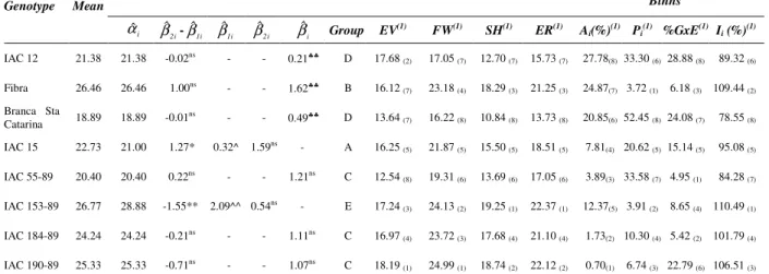
Concerning the methodology proposed by Toler and Burrows (1998), results in Table 1 showed that only the IAC 15 cultivar and the IAC 153-89 clone presented the _βˆ_{2i estimates different from}

i 1 ˆ

β , thus implying the choice of the bi-segmented

be more adapted to unfavorable environments (group D: βˆi < 1) or poor quality environments (Table 1). In this case, the indication should be restricted only to the producers with low, or no investment for crop management improvement. However, as these cultivars are destined to supply cassava for industrial sector in the northwestern region of Paraná state, because most of the producers that supply this segment have better technological conditions, the IAC 12 and Branca de Santa Catarina cultivars have no merit compared to the other genotypes assessed in the present study. In this context, the Fibra cultivar would be a good option to indicate for cropping in this region, if it was not for its high susceptibility to bacteriosis (Vidigal et al., 2000; Kvitschal et al., 2007). The IAC 55-89, IAC 184-89 and IAC 190-89 clones showed wide adaptation (βˆi = 1,0), that is, they tended not to present very discrepant yield means in function of the variations in the environmental quality (Table 1). This indicated

that these clones presented greater yield predictability that gave them agronomic merit equal to the IAC 15 cultivar, which showed a doubly favorable response pattern (Table 1). This was true, because the climatic conditions of the agricultural environments were unpredictable. On the other hand, greater importance should be given to the IAC 190-89 clone, because it has predictable phenotypic performance and, at the same time, surpassed the storage root yield means of the IAC 55-89 and IAC 184-89 clones and the IAC 15 cultivar (Table 1).

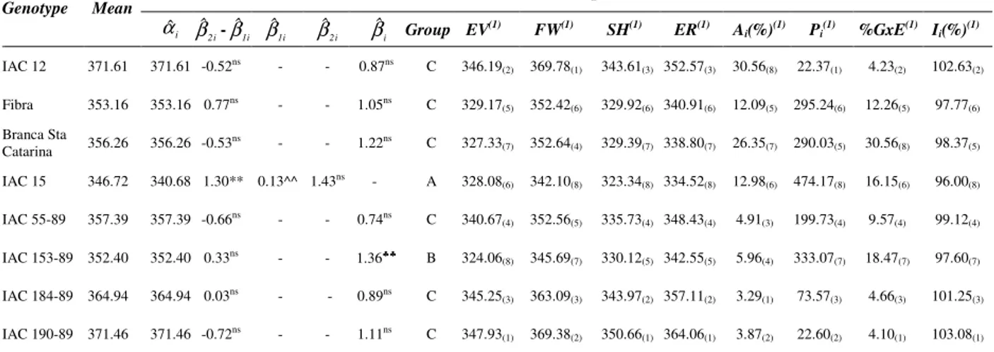
Regarding the storage root dry matter contents trait, it was observed that only the phenotypic response pattern of the IAC 15 cultivar was explained by the bi-segmented model (_βˆ_2i≠

i 1 ˆ

β ), as reported by Toler and Burrows (1998). This cultivar showed a convex and doubly desirable response pattern (Table 2). That is, as the environmental quality increased, this cultivar presented greater storage root dry matter content.

Table 1 – Resume of stability and adaptability analysis for storage root yield (t ha-1) of cassava genotypes, according to Toler and Burrows, Eskridge, AMMI analysis, Lin and Binns and Annicchiarico methodologies.

....…..….… Toler and Burrows ………... ……..……….. Eskridge ……… AMMI Lin and

Binns Annich. Genotype Mean

i

αˆ

i 2

ˆ

β -βˆ_1i βˆ_1i βˆ_2i βˆ_i Group EV(1) _FW(1) _SH(1) _ER(1) _A

i(%)(1) Pi(1) %GxE(1) Ii (%)(1) IAC 12 21.38 21.38 -0.02ns _{- - 0.21}♣♣ _{D 17.68}

(2) 17.05 (7) 12.70 (7) 15.73 (7) 27.78(8) 33.30 (6) 28.88 (8) 89.32 (6)

Fibra 26.46 26.46 1.00ns _{- - 1.62}♣♣ _{B 16.12}

(7) 23.18 (4) 18.29 (3) 21.25 (3) 24.87(7) 3.72 (1) 6.18 (3) 109.44 (2)

Branca Sta

Catarina 18.89 18.89 -0.01ns - - 0.49♣♣ D 13.64 (7) 16.22 (8) 10.84 (8) 13.73 (8) 20.85(6) 52.45 (8) 24.08 (7) 78.55 (8)

IAC 15 22.73 21.00 1.27* 0.32^ 1.59ns _{- A 16.25}

(5) 21.87 (5) 15.50 (5) 18.51 (5) 7.81(4) 20.62 (5) 15.14 (5) 95.08 (5)

IAC 55-89 20.40 20.40 0.22ns _{- - 1.21}ns _{C 12.54}

(8) 19.31 (6) 13.69 (6) 17.05 (6) 3.89(3) 33.58 (7) 4.95 (1) 84.28 (7)

IAC 153-89 26.77 28.88 -1.55** 2.09^^ 0.54ns _{- E 17.24}

(3) 24.13 (2) 19.25 (1) 22.37 (1) 12.37(5) 3.91 (2) 8.65 (4) 110.49 (1)

IAC 184-89 24.24 24.24 -0.21ns _{- - 1.11}ns _{C 16.97}

(4) 23.72 (3) 17.68 (4) 21.10 (4) 1.73(2) 10.30 (4) 5.42 (2) 101.79 (4)

IAC 190-89 25.33 25.33 -0.71ns _{- - 1.07}ns _{C 18.19}

(1) 24.99 (1) 18.74 (2) 22.12 (2) 0.70(1) 6.74 (3) 22.79 (6) 106.51 (3)

* and ** Significant at 5% and 1% of probability, respectively, by t test for H(_βˆ_2i=

i 1

ˆ

β ); ^ and ^^ Significant at 5% and 1% of probability, respectively, by t test for H(_βˆ_{1i= 1);} ♣♣ _{Significant at 1% of probability by t test for H(}

i

ˆ

β = 1); ns _{Not significant;} (1) _{The values inside the parenthesis indicate the ranking of stability in decreasing order; EV = safety-first index with variance}

Table 2 – Resume of stability and adaptability analysis for storage root dry matter content (g kg-1_{) of cassava}

genotypes, according to Toler and Burrows, Eskridge, AMMI analysis, Lin and Binns and Annicchiarico methodologies.

...….. Toler and Burrows …………... ….…..….. Eskridge ……… AMMI Lin and Binns Annich. Genotype Mean

i

αˆ

i 2

ˆ

β -βˆ_1i βˆ_1i βˆ_2i βˆ_i Group EV(1) _FW(1) _SH(1) _ER(1) _A

i(%)(1) Pi(1) %GxE(1) Ii(%)(1) IAC 12 371.61 371.61 -0.52ns _{- - 0.87}ns _{C 346.19}

(2) 369.78(1) 343.61(3) 352.57(3) 30.56(8) 22.37(1) 4.23(2) 102.63(2)

Fibra 353.16 353.16 0.77ns _{- - 1.05}ns _{C 329.17}

(5) 352.42(6) 329.92(6) 340.91(6) 12.09(5) 295.24(6) 12.26(5) 97.77(6)

Branca Sta

Catarina 356.26 356.26 -0.53ns - - 1.22ns C 327.33(7) 352.64(4) 329.39(7) 338.80(7) 26.35(7) 290.03(5) 30.56(8) 98.37(5)

IAC 15 346.72 340.68 1.30** 0.13^^ 1.43ns _{- A 328.08}

(6) 342.10(8) 323.34(8) 334.52(8) 12.98(6) 474.17(8) 16.15(6) 96.00(8)

IAC 55-89 357.39 357.39 -0.66ns _{- - 0.74}ns _{C 340.67}

(4) 352.56(5) 335.73(4) 348.43(4) 4.91(3) 199.73(4) 9.57(4) 99.12(4)

IAC 153-89 352.40 352.40 0.33ns _{- - 1.36}♣♣ _{B 324.06}

(8) 345.69(7) 330.12(5) 342.55(5) 5.96(4) 333.07(7) 18.47(7) 97.60(7)

IAC 184-89 364.94 364.94 0.03ns _{- - 0.89}ns _{C 345.25}

(3) 363.09(3) 343.97(2) 357.11(2) 3.29(1) 73.57(3) 4.66(3) 101.25(3)

IAC 190-89 371.46 371.46 -0.72ns _{- - 1.11}ns _{C 347.93}

(1) 369.38(2) 350.66(1) 364.06(1) 3.87(2) 22.60(2) 4.10(1) 103.08(1)

** Significant at 1% of probability by t test for H(_βˆ_2i=

i 1

ˆ

β ); ^^ Significant at 1% of probability by t test for H(_βˆ_{1i= 1);} ♣♣ Significant at 1% of probability by t test for H(_βˆ_i= 1); ns _{Not significant;}

(1) _{The values inside the parenthesis indicate the ranking of stability in decreasing order; EV = safety-first index with variance}

across environments as stability parameter; FW = safety-first index with Finlay and Wilkinson’s regression coefficient as stability parameter; SH = safety-first index with Shukla’s variance as stability parameter; and ER = safety-first index with Finlay and Wilkinson’s regression coefficient and Eberhart and Russel’s deviation of linear regression mean square as stability parameters.

The other genotypes in the genotype sets assessed a showed simple response pattern, implying the choice of the uni-segmented model by Digby (1979). Of these, only the IAC 153-89 clone showed specific adaptation to high quality environments (group B) for the storage root dry matter content trait (Table 2), while the other genotypes showed wide adaptability (group C: βˆi = 1,0). Thus, these genotypes tended to present little variation in the storage root dry matter content means whether submitted to favorable or unfavorable environments, respectively.

Regarding the methodology proposed by Eskridge (1990), the genotypes that showed greater storage root yield stability (types 2 and 3) were the IAC 190-89, IAC 153-89 and IAC 55-89 clones and the Fibra cultivar, because these clones presented the highest estimates of the safety first indexes (Table 1). For the storage root dry matter content trait, the IAC 190-89, IAC 184-89 IAC 55-89 clones and the IAC 12 cultivar showed greater stability in the types 2 and 3 (Table 2), according to Lin et al. (1986).

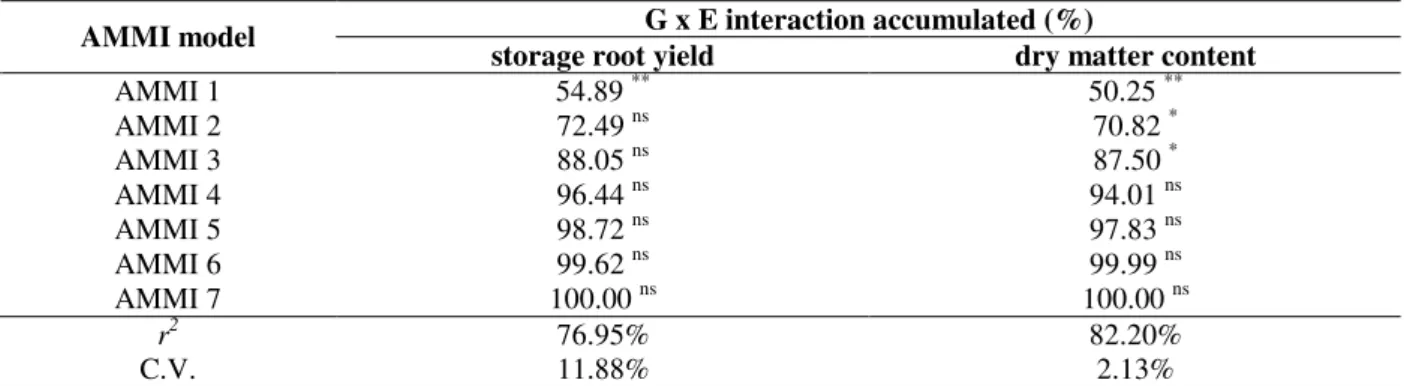
According to AMMI analysis, it would be important to emphasize that results found were partially different when comparing the yield and storage root dry matter content (Table 3). Seven PCA axis were needed to explain the total G x E interaction for both the traits. Besides, for the storage root yield, only the first PCA axis was significant and this one could explain only about 55.0% of total G x E interaction effect, while three PCA axes were significant for the dry matter content, being able to explain 87.5% of total G x E interaction effect. A goodness of the AMMI model fit was observed for the storage root dry matter content, which showed r2 over 82.2%, while r2 for

the storage roots yield was about 77.0% (Table 3). Since only the first PCA axis was significant for the storage root yield and the third PCA axis was significant for dry matter content, the Ai(%)

Table 3 - Summary of AMMI analysis for yield and storage root dry matter content of cassava genotypes. G x E interaction accumulated (%)

AMMI model

storage root yield dry matter content

AMMI 1 54.89 ** _50.25 **

AMMI 2 72.49 ns _70.82 *

AMMI 3 88.05 ns _87.50 *

AMMI 4 96.44 ns _94.01 ns

AMMI 5 98.72 ns _97.83 ns

AMMI 6 99.62 ns _99.99 ns

AMMI 7 100.00 ns _100.00 ns

r2 76.95% 82.20%

C.V. 11.88% 2.13%

* _and ** _{Significant at 5% and 1% of probability, respectively, by t test;} ns _{Not significant.}

For the storage root yield trait, the AMMI analysis classified the IAC 190-89, IAC 184-89 and IAC 55-89 clones and the IAC 15 cultivar as the most stable genotypes (Table 1), while for the storage root dry matter content the most stable genotypes were IAC 184-89, IAC 190-89, IAC 55-89 and IAC 153-89, respectively (Table 2). For both the characteristics assessed, the AMMI analysis indicated the IAC 12 cultivar as the most unstable. Regarding the methodologies proposed by Lin and Binns (1988) and Annicchiarico (1992), both the methodologies presented the same genotype classifying pattern for phenotypic stability, whether for the storage root production or for storage root dry matter content. Thus, the Fibra cultivar and the IAC 153-89, IAC 184-89 and IAC 190-89 clones showed greater storage root yield stability (Table 1), while the IAC 12 cultivar and the IAC 190-89, IAC 184-89 and IAC 55-89 clones presented greater stability for the storage root dry matter content (Table 2).

Further, to endeavor to understand the degree of association among the methodologies used in a more detailed manner, correlation analyses were applied among the stability parameter estimates of each methodology, which for the yield and storage root dry matter content are shown in Tables 4 and 5, respectively.

Regarding the storage root trait, it was observed that most of the methodologies applied considered the phenotypic means for selection of the most stable genotypes. This was confirmed by the significant correlations observed among the storage root yield means and the estimates of the respective parameters. Most of those stability parameters were positively correlated with the storage root yield means, except to the parameter

Pi, which was negatively correlated. Thus, the

genotypes presenting high mean tended to present

lower Pi estimates and, therefore were considered

the most stable. Similar results were obtained by Scapim et al. (2000) in corn. Rocha (2002) assessing the grain yield and oil content of soybean lines reported no association among the means and stability parameters ωi, S

2 di, r

2 _and

Ai(%) (ωi - Wricke, 1965; S 2

di, r 2

- Eberhart and

Russel, 1966; Ai(%) – AMMI analysis). It

indicated a certain difficulty in simultaneous selection of genotypes with high grain yield and high oil content that also presented good phenotypic stability.

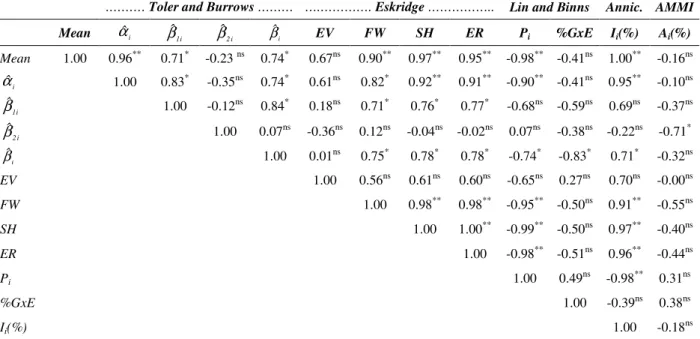
Regarding the methodology by Toler and Burrows (1998), no significant correlation was observed between the _βˆ_{1i and}

i 2 ˆ

β parameters that reinforced

the hypothesis that these parameters were really associated to the phenotypic response sensitivity of the genotypes to unfavorable and favorable environments, respectively.

The _βˆ_{1i parameter showed significant correlation}

only with the FW, SH and ER parameters reported

by Eskridge (1990). Although the βˆ1i parameter

presented high correlation estimates with the parameter proposed in the Lin and Binns (1998) and Annicchiarico (1992) methodologies, they were not significant (P > 0.05).

The _βˆ_{2i parameter showed significant correlation}

only with Ai(%) of the AMMI analysis, and this

was a negative value correlation (Table 4). This indicated that the IAC 15 cultivar, that presented concave response pattern (Table 1), showed a strong tendency to be more responsive to the improvements in environmental quality and was therefore more stable.

(1998) and Annicchiarico (1992) that indicated that the genotypes with higher βˆi estimates tended to be more stable. However, the βˆi parameter did not correlate with the

EV

parameter which might have occurred because the

EV

parameter only considered the variation among the environments as a measure of stability.

Table 4 - Resume of Pearson’s correlation analysis among phenotypic stability and adaptability parameters of cassava genotypes for storage roots yield (t ha-1).

.……… Toler and Burrows ……… ….…………. Eskridge ……….. Lin and Binns Annic. AMMI

Mean αˆi βˆ1i βˆ2i βˆi EV FW SH ER Pi %GxE Ii(%) Ai(%)

Mean 1.00 0.96** _0.71* _-0.23 ns _0.74* _0.67ns _0.90** _0.97** _0.95** _-0.98** _-0.41ns _1.00** _-0.16ns

i ˆ

α 1.00 0.83* _-0.35ns _0.74* _0.61ns _0.82* _0.92** _0.91** _-0.90** _-0.41ns _0.95** _-0.10ns

i 1 ˆ

β 1.00 -0.12ns _0.84* _0.18ns _0.71* _0.76* _0.77* _-0.68ns _-0.59ns _0.69ns _-0.37ns

i 2 ˆ

β 1.00 0.07ns _-0.36ns _0.12ns _-0.04ns _-0.02ns _0.07ns _-0.38ns _-0.22ns _-0.71*

i

ˆ

β 1.00 0.01ns _0.75* _0.78* _0.78* _-0.74* _-0.83* _0.71* _-0.32ns

EV 1.00 0.56ns 0.61ns 0.60ns -0.65ns 0.27ns 0.70ns -0.00ns

FW 1.00 0.98** 0.98** -0.95** -0.50ns 0.91** -0.55ns

SH 1.00 1.00** -0.99** -0.50ns 0.97** -0.40ns

ER 1.00 -0.98** -0.51ns 0.96** -0.44ns

Pi 1.00 0.49ns -0.98** 0.31ns

%GxE 1.00 -0.39ns 0.38ns

Ii(%) 1.00 -0.18ns

* _{Significant (P ≤ 0.05) by t test;} ** _{Significant (P ≤ 0.01) by t test;} ns _{Not significant.}

For this reason, Eskridge (1990) also emphasized that the EV parameter was not indicated for

stability studies under very contrasting

environmental conditions (Eskridge, 1990). Generally, it could be emphasized that regarding the storage root yield data, the methodology by Toler and Burrows (1998) was associated to the other methodologies, although it gave more detailed study of the G x E interaction and genotype adaptability.

According to the method proposed by Eskridge (1990), it was observed that the parameters estimates referring to the storage root yield stability were significantly correlated with each other, except for the EV parameter (Table 4).

Furthermore, theparameters FW, SH and ER were

negatively correlated with the parameter Pi of Lin

and Binns (1988), suggesting that genotypes with higher value of safety first index presented low Pi

estimates and, therefore, they were considered the most stable genotypes (Table 4). A positive

correlation was detected among the parameters

FW, SH and ER with the parameter Ii(%). Besides,

it was observed that the genotypes that showed

higher value of safety first indexes, also had higher

Ii(%) estimates and, therefore, could be considered

the most stable genotypes (Table 4).

The analysis proposed by Eskridge (1990) was able to assess G x E interaction in the storage root yield stability analysis of cassava genotypes, because high correlations were observed among its parameters and stability parameters of other methodologies applied in this study, which were Toler and Burrows (1998), Lin and Binns (1988) and Annicchiarico (1992).

According to AMMI analysis for the storage roots yield data set, it was observed that the Ai(%) did

not show significant correlation with any other methods applied, except to the parameter _βˆ_{2i of}

quality environments, a fact that justified the correlation observed among the βˆ2i and Ai(%)

parameters.

Table 5 shows the correlation estimates among the stability parameters referring to the storage root dry matter content. The greatest difference observed compared to the storage root yield data was by the methodology by Toler and Burrows (1998). The _βˆ_{1i and}

i

ˆ

β parameters for storage root yield presented significant correlations with the stability parameters in the methodologies by Eskridge (1990), Lin and Binns (1988) and Annicchiarico (1992) but did not show any correlation with the storage root dry matter contents data.

The _βˆ_{2i parameter that had presented significant}

correlation only with the Ai(%) parameter for the

storage root yield, presented significant correlation for the storage root dry matter content with the EV, Pi and Ii(%) parameters established by Eskridge

(1990), Lin and Binns (1988) and Annicchiarico (1992), respectively (Table 5). Although the βˆ2i

parameter did not present significant FW, SH and ER parameters, these correlations were negative

and high. That is, genotypes that presented high

i 2 ˆ

β estimates should present low EV, FW, SH, ER

and Ii(%) values, and high Pi values and were

therefore, unstable for the storage root dry matter content.

This showed the greater capacity of the Toler and Burrows (1998) methodology to detail the effects of the G x E interaction on the phenotypic expression, while the other methodologies did not give these interpretations.

However, since the Digby (1979) uni-segmented model was chosen for most of the genotypes, the

i 2 ˆ

β parameter might not have represented the true

dimension of the effect that the G x E interaction exercised on the storage root dry matter accumulation in the storage root of these genotypes.

The explanation for the differences observed in the correlation estimates among the stability parameters for the yield and storage root dry matter content could be related to the differentiated phenotypic response pattern of both the characteristics. Storage root yield showed a bi-segmented response (Table 1) for two genotypes (IAC 15 and IAC 153-89) while for storage root dry matter contents only one genotype presented its this bi-segmented pattern (Table 2).

Furthermore, genotype classification in the stability groups, according to Toler and Burrows (1998), showed greater variation compared to the storage root dry matter content data. For the storage root yield, the genotypes were distributed in all the five stability groups (A, B, C, D, E), while for the storage root dry matter content, the genotypes were placed in only three groups (A, B, C). This variation might have occurred in function of the smaller influence of the G x E interaction effects on the dry matter accumulation in the storage root and, consequently, a greater proportion of genotypes showed a strong tendency to a wide adaptability pattern (group C). Thus, the data set for the storage root yield was shown to be more suitable when comparing the Toler and Burrows (1998) methodology with the others. On the other hands, although the AMMI analysis has been reported as a really powerful tool on G x E interaction studies (Duarte and Vencovsky, 1992), some authors (Gauch and Zobel, 1988; Yau, 1995) have reported that it also has its limitations. While for the storage root yield, only the PCA axis was added to the AMMI model chosen, for the storage root dry matter content, three PCA axes were added to the respective AMMI model (Table 3). With this, the AMMI analysis consumed many degrees of freedom and that might have aggregated a very high quantity of noise to the SS(GxE), that was not interesting. It

would be important to state that Duarte and Venkovsky (1992) emphasized that the objective of the AMMI analysis was to recover only the part of the G x E interaction that was due to the main effects (genotypes and environments) relegating at the same time, the SS(GxE) part that was due to error

(noise). Therefore, a reasonable explanation for the absence of significant correlation among between βˆ2i and Ai(%) for the storage root dry

matter content could be related to the high proportion of noise aggregated to the AMMI3 model. Borges et al. (2000), by using AMMI analysis on studying of G x E interaction in common bean cultivars, reported three significant PCA axes, which represented nearly 63% of the total SS(GxE). These authors reported that AMMI

common bean cultivars assessed. However, when possible to capture a great pattern of G x E interaction, the AMMI analysis allowed an easy interpretation of the results by using biplot graphs. Thus, the plant breeders could easily select the specifically adapted genotypes to specific environments from a biplot graph, which could be more difficult by using other methodologies. Regarding the correlation among the stability parameters proposed by Eskridge (1990), Lin and Binns (1988) and Annicchiarico (1992) for the storage root dry matter content, it was observed that the correlation patterns were very similar to those observed for the storage root yield, i.e., these methodologies presented a high degree of association.

It was shown that all the methodologies applied were suitable for studying the phenotypic stability

in cassava clones and cultivars, as long as the peculiarities of each one were respected.

Thus, it could be inferred that the methodology by Eskridge (1990) could also be used as a tool in the analysis of phenotypic stability of cassava genotypes, although this methodology was more indicated for situations similar to those appropriate for the use of the methodologies by Eskridge (1990), Lin and Binns (1988) and Annicchiarico (1992). This was justified by the fact that the parameters estimated by these methodologies showed satisfactory correlation levels among each other and also with the storage root dry matter content data (Table 5). These methodologies were also satisfactory options when a good fit of the nonlinear regression model (Toler and Burrows, 1998) could not be obtained or the multiplication analysis (AMMI) could not be applied to the data set.

Table 5 - Resume of Pearson’s correlation analysis among phenotypic stability and adaptability parameters of cassava genotypes for storage root dry matter content (g kg-1_).

……….. Toler and Burrows ……… ...………….. Eskridge ……….. Lin and Binns Annic. AMMI

Mean αˆi βˆ1i βˆ2i βˆi EV FW SH ER Pi %GxE Ii(%) Ai(%)

Mean 1.00 0.99** 0.57ns -0.71* -0.05ns 0.89** 0.99** 0.96** 0.90** -0.98** -0.65ns 1.00** 0.12ns

i ˆ

α 1.00 0.66ns _-0.71* _0.05ns _0.85** _0.97** _0.95** _0.89** _-0.99** _-0.60ns _0.98ns _-0.10ns

i 1 ˆ

β 1.00 -0.47ns _0.59ns _0.27ns _0.50ns _0.52ns _0.49ns _-0.56ns _0.10ns _0.55ns _0.11ns

i 2 ˆ

β 1.00 0.43ns _-0.80* _-0.68ns _-0.67ns _-0.63ns _0.74* _0.45ns _-0.71* _-0.12ns

i

ˆ

β 1.00 -0.44ns _-0.08ns _-0.06ns _0.06ns _0.08ns _0.49ns _-0.06ns _0.01ns

EV 1.00 0.89** 0.92** 0.90** -0.91** -0.83* 0.91** -0.11ns

FW 1.00 0.94** 0.88** -0.97** -0.67ns 0.98** 0.14ns

SH 1.00 0.99** -0.97** -0.75* 0.98** -0.17ns

ER 1.00 -0.93** -0.77* 0.93** -0.32ns

Pi 1.00 0.70ns -0.98** -0.01ns

%GxE 1.00 -0.69ns 0.34ns

Ii(%) 1.00 0.04ns

* _{Significant (P ≤ 0.05) by t test;} ** _{Significant (P ≤ 0.01) by t test;} ns _{Not significant.}

Furthermore, in situations where the breeder wished only to make a prior and less detailed analysis of the genotype set available, or when the trait in question was not so affected by the G x E interaction as the storage root yield, methodologies such as those by Eskridge (1990), Lin and Binns (1988) and Annicchiarico (1992) could also be viable options. This is because they are more practical for the application of statistical analysis and for results interpretation. Furthermore, the

methodology proposed by Eskridge (1990) allows the researcher to choose the parameters that best satisfy the type of stability he wants to consider in the genotype selection, as reported by Lin et al. (1986).

specific adaptations of the genotypes, whether in high or low quality environments.

On the other hand, the AMMI analysis also showed some peculiarities that should be considered in its choice for application in the stability analyses of the cassava crop. First, there should be a good fit of the mathematical model to the data set available. In addition, it is essential that few PCA axles should be inserted to the respective AMMI model chosen. If these additional factors are respected, the AMMI analysis also permits an easy visualization of the specific interactions among genotypes and environments, by plotting the specific biplot graphs (Duarte and Venkovsky, 1992). Given this high capacity of specific interaction identification of the AMMI analysis, its use is suggested simultaneously with the Toler and Burrows (1998) methodology, a recommendation also made by Ferreira et al. (2006).

ACKNOWLEDGEMENTS

The authors thank Pinduca Indústria Alimentícia Ltda, Capes, CNPq for the financial support, and the lecturers, staffs, graduating and post-graduating students by Maringá State University (UEM) who helped to carry out this study.

RESUMO

O objetivo deste trabalho foi comparar diferentes metodologias de análise de estabilidade fenotípica considerando produção e teor de matéria seca nas raízes tuberosas de oito genótipos de mandioca, avaliados em oito ambientes na região Noroeste do Paraná. Todas as metodologias aplicadas se mostraram aptas no estudo da estabilidade dos genótipos avaliados, cada uma delas com suas particularidades. As metodologias de Eskridge, Annicchiarico e Lin e Binns se mostraram mais adequadas para situações de menor efeito da interação G x A. A análise AMMI e a metodologia de Toler e Burrows propiciaram um melhor detalhamento das adaptações específicas dos genótipos a ambientes favoráveis e desaforáveis. É sugerido o uso simultâneo da análise AMMI e da metodologia de Toler e Burrows. O clone IAC 190-89 mostrou-se mais promissor.

REFERENCES

Annicchiarico, P. (1992), Cultivar adaptation and recommendation from alfafa trials in Northern Italy. Journal of Genetics and Plant Breeding, 46, 269-278. Borges, L. C.; Ferreira, D. F.; Abreu, A. F. B. and Ramalho, M. A. P. (2000), Emprego de metodologias de avaliação da estabilidade fenotípica na cultura do feijoeiro (Phaseolus vulgaris L.). Revista Ceres

47(269), 89-102.

Cruz, C. D. (2001), Programa Genes: aplicativo computacional em genética estatística. UFV, Viçosa, 642p.

Cruz, C. D. and Regazzi, A. J. (2001), Modelos Biométricos Aplicados ao Melhoramento Genético – 2ed. rev., UFV, Viçosa, 309p.: il.

Cubero, J. I. and Flores, F. (1994), Métodos estadísticos para estudo de la estabilidad varietal em ensayos agrícolas. Junta de Andalucía, Sevilla, 176p. (monografías, 12/94).

Digby, P. G. N. (1979), Modified joint regression analysis for incomplete variety x environment data. Journal of Agricultural Sciences, 93, 81-86.

Duarte, J. B. and Vencovsky, R. (1999), Interação Genótipos x Ambientes: Uma introdução à análise “AMMI”. FUNPEC, Ribeirão Preto, 60p. (série monografias, 9).

Eberhart, S. A. and Russel, W. A. (1966), Stability parametrs for comparing varieties. Crop Science, 6, 36-40.

Embrapa (1999), Sistema Brasileiro de Classificação de Solo. EMBRAPA-CNPS, Rio de Janeiro, 180p. Eskridge, K. M. (1990), Selection of stable cultivars

using a safety-first rule. Crop Science,30, 369-374. Ferreira, D. F. and Zambalde, A. L. (1997),

Simplificação das análises de algumas técnicas especiais da experimentação agropecuária no Mapgen e softwares correlatos. In: Congresso da Sociedade Brasileira de Informática Aplicada à Agropecuária e Agroindústria, 1997. Anais... SBI, Belo Horizonte, 285-291.

Ferreira, D. F.; Demétrio, C. G. B.; Manly, B. F. J.; Machado, A. A. and Venkovsky, R. (2006), Statistical models in agriculture: Biometrical methods for evaluating phenotypic stability in plant breeding. Cerne, 12(4), 373-388.

Finlay, K. W. and Wilkinson, G. N. (1963), The analysis of adaptation in a plant-breeding programme. Australian Journal Agriculture Resource, 14, 742-754.

Fukuda, W. M. G. (1996), Estratégia para um programa de melhoramento genético de mandioca. Embrapa-CNPMF, Cruz das Almas, 35p. (Embrapa-CNPMF. Documentos, 71).

Gauch Jr, H. G. (1988), Model selection and validation for yield trials with interaction. Biometrics, 44, 705-716.

Gauch Jr, H. G. and Zobel, R. W. (1988), Predictive and postdictive success of statistical analysis of yield trials. Theoretical and Applied Genetics, 76(1), 1-10. Grosmann, J. and Freitas, A. G. (1950), Determinação

do teor de matéria seca pelo peso específico em raízes de mandioca. Revista Agronômica, 14, 75-80. Kataoka, S. (1963), A stochastic programming model.

Econometrica,31, 181-196.

Kawano, K. (2003), Thirty years of Cassava Breeding for productivity – Biological and Social Factors for Success. Crop Science, 43, 1325-1335.

Kvitschal, M. V. (2003), Avaliação da estabilidade e da adaptabilidade de clones de mandioca (Manihot esculenta Crantz). MSc. Thesis, Universidade Estadual de Maringá, Maringá, 141p.

Kvitschal, M. V.; Vidigal Filho, P. S.; Scapim, C. A.; Gonçalves-Vidigal, M. C.; Pequeno, M. G.; Sagrilo, E. and Rimoldi, F. (2007), Evaluation of phenotypic stability of cassava clones by AMMI analysis in northwestern Paraná state. Crop Breeding and Applied Biotechnology, 6, 236-241.

Lin, C. S. and Binns, M. R. (1988), A superiority measure of cultivar performance for cultivar x location data. Canadian Journal of Plant Science, 68, 193-198.

Lin, C. S.; Binns, M. R. and Lefkovitch, L. P. (1986), Stabillity analysis: Where do we stand? Crop Science,

26, 894-900.

Nunes, G. H. S.; Elias, H. T.; Hemp, S. and Souza, M. A. (1999), Estabilidade de cultivares de feijão-comum no Estado de Santa Catarina. Revista Ceres,

46(268), 625-633.

Pimentel Gomes, F. (1990), Curso de estatística experimental. Nobel, Piracicaba, 401p.

Rocha, M. M. (2002), Seleção de linhagens experimentais de soja para adaptabilidade e estabilidade fenotípica. Dr. Thesis, Escola Superior de Agronomia Luiz de Queiroz – Universidade de São Paulo, Piracicaba, 173p.

Sagrilo, E.; Vidigal Filho, P. S.; Pequeno, M. G.; Gonçalves-Vidigal, M. C. and Kvitschal, M. V. (2008), Dry matter production and distribution in three cassava (Manihot esculenta Crantz) cultivars during the second vegetative cycle. Brazilian Archives of Biology and Technology, 51 (6), 1079-1087.

Sagrilo, E.; Vidigal Filho, P.S.; Pequeno, M. G.; Scapim, C. A.; Gonçalves-Vidigal, M. C.; Diniz, S. P. S. S.; Modesto, E. C. and Kvitschal, M. V. (2003), Effect of harvest period on the quality of storage roots and protein content of the leaves in five cassava cultivars (Manihot esculenta Crantz). Brazilian Archives of Biology and Technology, 46, 295-305. Scapim, C. A.; Oliveira, V. R.; Braccini, A. L.; Cruz, C.

D.; Andrade, C. A. B. and Gonçalves-Vidigal, M. C. (2000), Yield stability in maize (Zea mays L.) and correlations among the parameters of the Eberhart e Russel, Lin e Binns and Huehn models. Genetics and Molecular Biology, 23, 387-393.

Shukla, G. K. (1972), An invariant test for the homogeneity of variances in a two-way classification. Biometrics, 28, 1063-1072.

Statical Analisys System Institute (1997), SAS/STAT software: changes and enhancements through release 6.12 (software). SAS Institute, Cary, 1116p. +1cd. Toler, J. E. and Burrows, P. M. (1998), Genotypic

performance over environmental arrays: a non-linear grouping protocol. Journal of Applied Statistics,

25(1), 131-143.

Vendruscolo, E. C. G. (1997), Comparação de métodos de avaliação de adaptabilidade e estabilidade de genótipos de milho pipoca (Zea mays, L.) na região Centro-Sul do Brasil. MSc. Thesis, Universidade Estadual de Maringá, Maringá, 84p.

Vidigal Filho, P. S.; Pequeno, M. G.; Scapim, C. A.; Gonçalves-Vidigal, M. C.; Maia, R. R.; Sagrilo, E.; Simon, G. A. and Lima, R. S. (2000), Avaliação de cultivares de mandioca na região noroeste do Paraná. Bragantia, 59(1), 69-75.

Wricke, G. (1965), Zur berechning der okovalenz bei sommerweizen und hafer. Pflanzenzuchtung, 52, 127-138.

Yau, S. K. (1995), Regression and AMMI analyses of genotype x environment interactions: An empirical comparison. Agronomy Journal, 87, 121-126.

Zobel, R. W.; Wright, A. J. and Gauch Jr., H. G. (1988), Statistical analysis of a yield trial. Agronomy Journal, 80, 388-393.