Technological adoption in health care - The role of
payment systems
∗Pedro Pita Barros Universidade Nova de Lisboa
and CEPR (London)
Xavier Martinez-Giralt Universitat Aut`onoma de Barcelona
and MOVE
October 2013
Abstract
This paper examines the incentive to adopt a new technology given by some popular reimbursement systems, namely cost reimbursement and DRG reimbursement. Adoption is based on a cost-benefit criterion. We find that retrospective payment systems require a large enough patient benefit to yield adoption, while under DRG, adoption may arise in the absence of patients benefits when the differential reimbursement for the old vs. new technology is large enough. Also, cost reimbursement leads to higher adoption under some conditions on the differential reimbursement levels and patient bene-fits. In policy terms, cost reimbursement system may be more effective than a DRG payment system. This gives a new dimension to the discussion of prospective vs. retrospective payment systems of the last decades centered on the debate of quality vs. cost containment.
Keywords:
JEL numbers: I11, I12
CORRESPONDENCE ADDRESSES:
Pedro Pita Barros, Nova School of Business and Economics, Universidade Nova de Lisboa, Campus de Campolide, PT-1099-032 Lisboa, Portugal; email: [email protected]
Xavier Martinez-Giralt, CODE, Edifici B, Universitat Aut`onoma de Barcelona, 08193 Bellaterra, Spain; email: [email protected]
1
Introduction.
Recent decades have witnessed an increasing share of the level of spending on
health care relative to the GDP (see OECD, 2005a,b). There is a general
con-sensus that technological development (and diffusion) is a prime driver of this
phenomenon. The recent account by Smithet al. (2009) estimates that medical
technology explains a fraction of between 27-48% (depending on different
esti-mation techniques) of growth in the US health spending in the period 1960-2007.
Despite the relatively large literature documenting empirically the impact of
inno-vation in health care, a theoretical corpus has not been fully developed yet. In this
paper we address a particular theoretical issue: the relationship between payment
systems and the rate of technology adoption. To avoid unnecessary confusion, let
us point out that we refer to adoption as the decision of a provider to acquire a
piece of new technology available. We do not consider the process by which such
a new technology has become available, nor the R&D involved in it, nor any other
considerations. Our departing point is that a new way to provide some treatment
has become available, and thus providers must decide whether to acquire it.
We contribute to the theoretical literature by setting up a model of uncertain
demand, where the novelty lies in relating the technological shift to the increased
benefit for patients, financial variables, and the reimbursement system to providers.
We seek to assess the impact of the payment system to providers on the rate of
tech-nology adoption. We propose two payment schemes, a reimbursement according
to the cost of treating patients, and a DRG payment system where the new
technol-ogy may or may not be reimbursed differently from the old technoltechnol-ogy. We find
that under a cost reimbursement system, large enough patient benefits are
neces-sary for adoption to occur. However, when the DRG offers a higher reimbursement
for new technology, adoption occurs even in the absence of patients’ benefits. In
this case, the new technology must be reimbursed sufficiently higher than the old
one. Finally, to compare the levels of technological adoption in the differnt
pay-ment regimes, we take as reference an investpay-ment level yielding to the provider
reimbursement leads to higher adoption of the new technology if the rate of
reim-bursement is high relative to the margin of new vs. old DRG. Having larger patient
benefits favors more adoption under the cost reimbursement payment system,
pro-vided that adoption occurs initially under both payment systems. In policy terms,
it may well be the case that for some objectives of the regulator regarding the level
of technological adoption, a retrospective payment system to the providers is more
effective than a prospective reimbursement system. This opens again the
discus-sion of prospective versus retrospective payment systems in a wider framework
than the debate of quality vs. cost containment developed along the last decade.
To evaluate the impact of the adoption of new technology, we study how adjusting
the parameters of the payment function affect adoptionfor a given level of total
expenditure. We use this approach as a proxy for a welfare analysis of adoption,
due to the inherent difficulties in our model to define a social welfare function for
the health authority. We obtain that under risk neutrality, more cost reimbursement
always increases adoption. More generally, risk aversion leads to ambiguity of how
the level of adoption adjusts to changes in the payment system.
The structure of the paper is as follows. The following section provides a brief
overview of the literature addressing the impact of technological progress on health
care expenditures from a number of different perspectives. Section 3 introduces
the model and behavioral assumptions. Sections 4 and 5 deal with the adoption
decision of a new technology under the different payment regimes. Section 6
com-pares the levels of adoption across payment schemes. Section 7 studies whether
the different reimbursement regimes induce over- or under adoption with respect
to the first-best associated with the social welfare. A section with conclusions and
a technical appendix close the paper.
2
Literature review
In general, the main findings in the empirical literature can be grouped in three
related classes: (i) technological development induces an increase in health care
on the R&D effort, and (iii) the R&D effort determines the type of technological
development, either brand new technology, or improvements in existing
technolo-gies (or both). In contrast, our analysis as mentioned above, links the
reimburse-ment system to the adoption of a new technology. Some of the main conclusions
of this mainly empirical literature stress the fact that (a) prospective payment
sys-tems encourage cost efficient new technologies but have perverse effects on quality
improvement, and (b) retrospective payment systems encourage quality but dim
sensitivity toward cost efficiency.
Di Tommaso and Schweitzer (2005) collect a series of papers to describe the
benefits of promoting a country’s health industry as a way to stimulate its
high-technology industrial capacity. In particular, they stress the fact that the health
system is a major generator of scientific knowledge leading not only to
improve-ments in the health state of the country, but also produce positive externalities on
other industries in the form of public goods, “national champions” industries
pro-ducing new technological breakthroughs and high-technology start-ups that with
adequate protection will turn into self-sustaining industries.
According to the OECD (2005c), to understand the economic consequences of
technological change it is necessary to know “... whether the new technologies
sub-stitute for old or are add-ons to existing diagnostic and treatment approaches, (...)
whether these technologies are cost reducing. cost neutral, or cost effective, [and]
what the target population is” (p.28). As clear-cut as these questions may look,
they do not always lead to a simple answer. It may well occur that a
technologi-cal change allows for reducing the average cost, improving quality, and reducing
risk to patients. However, such technology would also allow for an expansion of
the population of patients suitable for such technology, thus inducing an increase
in the overall health care budget. Key determinants of the technological change
in health care systems (see OECD, 2005c: 31-38) are (i) the relationship between
health care expenditures and GDP; (ii) the reimbursement arrangements in the
in-surance contracts, and (iii) the regulatory environment.
technological advance “... but eventually [technological advance] drives costs up.
The imperative to innovate overcomes the effort to economize.” (p. 936).
In a fascinating paper, Weisbrod (1991) explains the interaction between the
R&D effort and the health care insurance system as the result of the combination
of two arguments. The first one tells us that health care expenditures are driven
by technical innovation, which in turn, is the result of the R&D processes, which
are determined by the (expected future) financial mechanisms allowing for
recov-ering the R&D expenses. These financial mechanisms are related to the expected
utilization of the new technologies, which is defined by the insurance system. The
second argument defines the present technological situation as a proxy for past
R&D effort and determines the demand for health care insurance. In this respect,
Weisbrod and LaMay (1999) elaborate on the increased uncertainty surrounding
the R&D decision process, as private and public insurance decisions on the use of
and payment for health care technology are under tighter control from the pressures
for cost containment.
In studying the sources of increasing health care expenditures, Foxet al.(1993)
point out three elements in the case of the United States. These are the view of
health insurance as a tax subsidy, the presence of entry barriers into the medical
profession, and the lack of competition in the insurance industry. Also, Chou and
Liu (2000) look at Taiwan’s National Health Insurance program to find evidence
of causality from third party payment mechanism inducing higher patient volume
that in turn, leads hospitals’ adoption of new technologies.
Cutleret al. (1998) go into the debate of the impact of the increase in health
care expenditures on health outcomes. In front of positions illustrated by Fuchs
(1974) or Newhouse and the Insurance Experiment Group (1993) where the main
conclusion is that medical care has little impact on health outcomes, Cutleret al.
(1998) argue that in a “dynamic context, the evidence that the marginal value of
medical care at a point in time is low does not imply that the average value of
med-ical technology changes over several decades is low. To measure cost-of-living
tech-nology changes.” (p. 133). So far there is no general agreement on how to
con-struct such indexes. On the one hand, hedonic prices are difficult to apply given
the widespread regulation of prices; on the other hand, there is no agreement on
how to set up a model of medical decision-making. Without such indexes, Cutler
et al. (1998) argue that no complete answer can be given to the question of the
consequences of the increase of health care expenditures on the health status of the
population.
In a somewhat similar perspective, Newhouse (1992) also calls for dynamic
arguments to analyze the impact of the increasing costs of medical care when
evaluating the welfare losses at a point in time as compared with those that may
arise due to the increases of expenditures over time. “However, I will contend that
economists have been too preoccupied with a one-period model of health care
ser-vices that takes technology as given, and that we need to pay more attention to
technological change.” (p.5).
The most detailed analyses of the benefits vs. costs of medical advances have
been performed on the basis of case studies. To mention some, the TECH team is
exploring whether individuals living in countries that rapidly adopted new
revas-cularization technologies and clot-dissolving drugs are more likely to survive heart
attacks than individuals living in countries that adopted such interventions more
slowly. McClellan and Kessler for the TECH group (1999) show the spread of
health technology in 16 OECD nations with widely divergent health care systems,
using treatment of heart attacks. TECH (2001) update the information and
re-port that technological change has occurred in all 17 countries of the study, but
its diffusion shows very different rates. For intensive procedures, countries can be
classified into three patterns: early start and fast growth; late start/fast growth; and
late start/slow growth. Those differences are attributed to economic and regulatory
incentives in the health care systems.
Duggan and Evans (2005) estimate the impact of medical innovation in the case
of HIV antiretroviral treatments in the period 1993-2003 from a sample of more
The authors evaluate the cost effectiveness of new drugs on spending. They
con-clude that those new drugs yield a three-fold increase in lifetime Medicaid
spend-ing due to their high cost and increase in life expectancy. Despite this, the authors
conclude that the new treatments were cost effective based on the value of a year
of life.
Cutler and Huckman (2003) study the diffusion of angioplasty in New York
state to address the puzzling feature of many medical innovations that
simultane-ously reduce unit costs and increase total costs. The key elements of their analysis
is the identification of the so-called treatment expansion (the provision of more
in-tensive treatment to patients with low-grade symptoms) and treatment substitution
(the shift of a patient from more- to less-intensive interventions), and the
consider-ation of the costs and benefits of these effects not only at a point in time but also
their change over time.
Bokhari (2008) studies the impact on adoption of cardiac cauterization
labora-tories according to HMO market penetration and HMO competition. In a related
line, Baker (2001) analyses HMO market penetration and diffusion of MRI
equip-ment, and Baker and Phibbs (2002) look at HMO market penetration and diffusion
of neonatal intensive care units.
Finally, Cutler and McClellan (2001) look at treatments for heart attack, low
birthweight infants, depression, and cataracts. Taking into account the treatment
substitution and treatment expansion effects, they conclude that the estimated
ben-efit of technological change is much greater than the cost.
The findings advanced in the empirical literature link health care expenditure
and technology diffusion based on a number of factors, including (i) the degree
of substitutability/complementarity between the old and new technologies, (ii) the
efficiency of the innovation in terms of effort reduction and output improvement,
(iii) the impact of expenses of the adoption of new technologies in accordance
with the treatment expansion and treatment substitution effects, (iv) the presence
of agents whose objective functions need not be profit maximization, and (v) the
These and other elements determine the incentives to develop and diffuse new
medical technologies. However, there are very few theoretical models providing
support to the empirical modeling, and allowing for addressing the incentives for
technological development, the rate of its diffusion in the health care system, or the
welfare effects of the adoption of such (expensive) medical innovations. Among
those few contributions we find Goddeeris (1984a,b), Baumgardner (1991), and
Selder (2005), who examine the effects of technical innovation on the insurance
market, and Miraldo (2007) who studies the feed-back effects between the health
care and the R&D sectors, Grebel and Wilfer (2010) who study the diffusion of
two competing technologies, and Levaggi et al. (2012) who consider how the
uncertainty on patients’ benefits affects the incentives to invest in new technologies.
Goddeeris (1984b) develops a framework for analyzing the effects of medical
insurance on the direction of technological change in medicine, where research is
carried out by profit maximizing institutions. Goddeeris (1984a) sets up a dynamic
model to look at the welfare effects of the adoption of endogenously supplied
in-novations in medical care financed through medical insurance, using as welfare
criterion the expected utility of the typical individual. Baumgardner (1991) builds
upon Godderis (1984a) and studies the relationship between different types of
tech-nical change, welfare and different types of insurance contracts, to conclude that
the value of a specific development in technology depends on the type of
insur-ance contract. Selder (2005) extends Baumgardner (1991), analyzing the
incen-tives of health care providers driven by different reimbursement systems to adopt
new technologies in a world with ex-post moral hazard and their impact on the
rate of diffusion. In particular, he considers a model where “the physician chooses
a technology and offers this technology to the patient. The patient then chooses
the treatment intensity which maximizes his utility given the technology offered.
Taking these actions into account, the insurer (or social planner) designs a
remu-neration scheme for the physician and an insurance contract for the patient. He
cannot contract upon technology choice and treatment intensity” (p. 910). The
Miraldo (2007) studies the impact of different payment systems on the
adop-tion of endogenously supplied new technologies, by introducing a feed-back effect
from the health care sector into the R&D sector. Her central claim is that “[t]he
diffusion process of existing technologies may feed back into the R&D sector since
the incentives to create new technologies depend on the propensity to apply them”
(p.2). In turn, the expected profitability of a newly developed technology depends
on the number of hospitals adopting (market size) and the reimbursement
associ-ated with it. R&D activities may be done in either in-house or externally. Both
scenarios are solved for the technologies’ optimal quality and cost decreasing
lev-els and for the decision on optimal reimbursement by a central planner.
Grebel and Wilfer (2010) study the diffusion process of two competing
tech-nologies in the health care sector where network externalities and individual
learn-ing are the main decision drivers. In particular, the demand side of the market
(physicians) learn by using the new technologies and generate network
externali-ties that diffuse the information of the new technologies and thus affects the
de-cision of adopting. On the supply side, firm size and the time to market play an
important role. These forces, namely the willingness of potential technology users
to adopt a new technology and the strategic behavior of the firm, subject to the
network externalities, shape the resulting market structure.
Levaggiet al. (2012) is the closest contribution in spirit to our modeling
ap-proach. They analyze the interaction between different payments systems and the
uncertainty of patients’ benefits on the incentives for providers to invest in new
technologies, both in terms of static efficiency (cost reduction) and dynamic
ef-ficiency(timing of adoption). It turns out that if lump-sum payments cannot be
implemented (which often occurs in the real world health care systems), there
ap-pears a trade-off between both types of efficiency, because the incentive to adopt
the new technology when the price equals the marginal cost (yielding static
effi-ciency) yields a later-than-efficient adoption timing. In contrast, we focus in the
impact of the design of the reimbursement system on the incentives to adopt a new
There are several relevant topics that we do not address in our analysis. One is
the role of the malpractice system, with extra tests and procedures ordered in
re-sponse to the perceived threat of medical malpractice claims (Kessler and
McClel-lan, 1996). On the effects of hospital competition on health care costs see Kessler
and Mcclellan (2000). Another topic is the use of technology assessment
crite-ria to measure the value of new health care technologies brought about by R&D
investments. Economic evaluation (cost-benefit analysis) of new technologies is
common in pharmaceutical innovation and has led to a wide body of literature,
both on methodological principles and on application to specific products. For a
recent view on the interaction between R&D and health technology assessment
criteria, see Philipson and Jena (2006).
Most of our analysis is set in the context of a health care sector organized
around a NHS. We do not explicitly account for a specific role of the private sector
in the provision of health care services as a driver in the diffusion of new available
technologies. Our analysis is applicable to both private and public sectors to the
extent that they use the payment mechanisms we explore below.
3
The model
We consider a semi-altruistic provider, who values financial results (represented by
an increasing and concave utility function,V(·), V′(·) > 0 and V′′(·) < 0) and
patients’ health gains. We will refer to the hospital as an example of a relevant
provider throughout the text.
There is a potential total number of homogeneous patients (i.e. they all suffer
from the same illness and with the same severity)q∗ in need of treatment.1 The
actual number of patients treated by the hospital,q, is uncertain over the course of
a time period (say, a year). The hospital can install a new technology that allows
it to treatq¯patients. If demand for hospital services exceeds the newly installed
1Allowing for heterogenous patients in terms of severity levels should not alter the qualitative
capacity, then patients are treated using an older technology. In other words, the
new technology is used prior to the old technology. We assume that within the set of
patients needing treatment no prioritization is made across patients.2 Uncertainty
about demand for hospital services is modeled simply as distributionF(q), with
densityf(q), in the domain[0, q∗].
Note that we model adoption of a new technology as an investment decision
in capacity to treat patients. That is, adoption is represented by a continuous
en-dogenous variable q¯. In this sense we interpret the new technology in terms of
the health care services it provides rather than as a discrete decision on whether
to adopt or not. Accordingly, adoption in our context means an investment in
ca-pacity to treat patients with a different protocol yielding higher benefits to them.
Alternatively, we can think of one decision, namely to adopt or not to adopt, and
at the same time decide the scale of the adoption. In this case, the new technology
can be a (scalable) equipment or training of health professionals in providing a new
treatment.
We also assume that uncertainty is symmetric for the two technologies. In other
words, we assume the the total number of patients is uncertain, not how many
treatments will be required with the new technology. Implicitly, this implies the
the new technology represents a step forward in the development of the treatment
rather than a break through improvement.
Finally, we also consider the patients’ benefits as the criterion for the use of the
new technology. Patients are treated with the new technology up to capacity, and
if there is demand left, it is treated with the old technology. This is a simple
mech-anism that in our context of homogeneous patients is meaningful. More general
set-ups where patients are differentiated in severity allow for more sophisticated
mechanisms (see Siciliani, 2006, and Hafsteinsdottir and Siciliani, 2010 for the
analysis of treatment selection mechanisms when patients differ in severity).
Hospitals receive a payment transfer R. Such payment may be prospective,
retrospective, or mixed. We will analyze two payment systems. On the one hand,
2This is assumed for expositional simplicity. The problem remains basically the same within each
we will study a cost reimbursement scheme flexible enough to accommodate total
cost reimbursement, fixed fee/capitation, and partial cost reimbursement. On the
other hand, we look at the effects of a DRG-based payment system with payments
by sickness episode.3 We assume that the payer can commit to the rule announced.
Otherwise, “hold-up” issues `a la B¨os and de Fraja (2002) could arise.
The new technology has an investment cost per patient treated ofp.4 There is
also a constant marginal cost per patient treated, given byθin the new technology
and bycin the old technology. Accordingly, the total cost is composed of (i) the
cost of installing the new technology allowing to treat up toq¯patients given bypq¯,
and (ii) the cost of treatments. This in turn, depends on whether realized demand
is below capacity (in which case it is given byθq), or whether realized demand is
above capacity. Then,q¯patients are treated with the new technology at marginal
costθ, and(q−q¯)patients are treated under the old technology with marginal cost
c. Formally, the total cost function of the hospital is given by,
T C=
(
pq¯+θq ifq ≤q¯
pq¯+θq¯+c(q−q¯) ifq >q¯ (1)
We assume that the average and marginal costs of the new technology is higher
than the corresponding average and marginal costs of the old technology:
Assumption 1.
p+θ−c >0. (2)
With this assumption we capture the generally accepted claim that new
tech-nologies are not cost savers relative to existing ones and are one of the main drivers
of the cost inflation in the health care sectors in developed countries.
The endogenous character of q¯leads us to assume that q¯is not contractible
(as in the literature). The specific way the hospital will use the new technology
3
Implicitly we define DRGs as describing processes and procedures. We have chosen this ap-proach instead of the alternative definition of DRGs capturing the casemix, as we find it more suitable for our analysis.
4This means that for the purposes of our main arguments we abstract from the potential lumpiness
depends on elements internal to the provider such as the clinical decision-making.
In this sense, the model can be interpreted as conveying private information and
the payer trying to induce socially optimal decisions through the choice of the
reimbursement system.
Patient benefits measured in monetary units are given bybunder the new
tech-nology and byˆbin the old technology. We assumeb > ˆb, b > p+θandˆb > c,
so that it is socially desirable to provide treatment to patients. To ease notation,
hereafter let∆ ≡ b−ˆb. That is ∆represents the incremental patients’ benefits
when treated with the new technology.
Economic evaluation criteria will often require that incremental benefits from
the new technology exceed incremental costs, that is:
Assumption 2. Economic evaluation criterion for approval of new technology
re-quires incremental benefits greater than incremental costs from the new technology.
That is,
∆> p+θ−c >0 (3)
Hereinafter, whenever we mention that economic evaluation criteria (or health
technology assessment) is used, we mean that incremental benefits are greater than
incremental costs (or equivalently Assumption 2 holds).5
The expected welfare for the hospital decision maker is given by the valuation
of the financial results of the hospital and by valuation of patients’ benefits from
treatment.
W =
Z q¯
0
V(R−pq¯−θq)f(q)dq+
Z q∗
¯
q
V(R−pq¯−θq¯−c(q−q¯))f(q)dq
+η
Z q¯
0
bqf(q)dq+η
Z q∗
¯
q
(q−q¯)ˆb+ ¯qbf(q)dq (4)
5We assume new technologies that are both cost and benefit incremental. The relevant assumption
This function captures a semi-altruistic provider who weights its private
ben-efits and the social benben-efits implicitly through the functionV and the parameter
η > 0. In particular, the financial result of the hospital is given by revenues R
(that will follow a pre-specified rule), minus the costs of treating patients. Costs
of the hospital have two components. First, the cost of installing the new
technol-ogy allowing to treat up toq¯patients. This is given bypq¯, regardless of whether
demand exceeds or not, the capacity level of the new technology. Second, there is
the cost of actual treatments when realized demand is below the capacity built for
the new technology. This cost isθq. On the other hand, when realized demand is
above the capacity available for treatment under the new technology,q¯patients are
treated with the new technology at marginal costθ, and(q−q¯)patients are treated
under the old technology with marginal costc. Financial results are assessed by the
hospital with a utility functionV. This valuation of financial results corresponds
to the first line of equation (4).
The other element of the welfare function of the hospital is made up of benefits
to patients. These are b andˆb in the event of treatment under the new and old
technology respectively. When realized demand is below the capacity level of the
new technology, then utilitybqis generated for each level of realized demand. In
the case of realized demand above the capacity level for the new technology, q¯
patients have utilityband(q−q¯)patients have utilityˆb. The expected utility over
all possible levels of realized demand is the second line of equation (4). Note also
that in the computation on the expected welfare we are summing over probabilities,
not over patients. Finally, we assume that provider’s altruism translates in a higher
weight on patients’ welfare than in the financial results.
The (adoption) decision problem of the hospital is to choose the level q¯of
patients to be treated under the new technology. Naturally, such decision is
contin-gent on the system of reimbursement to the hospital.6 We will study and compare
a (partial) cost reimbursement system and a DRG payment system.7
6
Abbey (2009) presents a general appraisal of health care payment systems. See also Culyer and Newhouse (2000).
7
Note that the question that we tackle isnotthe design of an optimal payment
system to incentivate adoption, but the study the impact of some popular
reim-bursement systems (see Mossialos and LeGrand, 1999) on the level of adoption of
new technology.
To clarify the intuition behind some of the results, we illustrate their content
with a restricted version of the model characterized by risk-neutrality and a uniform
distributionq∗ = 1. These are referred to in the text as remarks.
4
Technology adoption under cost reimbursement
Let us assume that the hospital is reimbursed according to the cost of treating
pa-tients. We want to characterize the optimal choice of q¯by the hospital decision
maker, taken as given the payment system.
The total cost depends on the level of realized demand and is defined as the
fixed cost of investment in the new technology (pq¯) and the variable cost given by
the population of patients treated. We have to distinguish two situations according
to whether or not realized demand is in excess of the capacity provided by the
new technology (q¯). Whenever the installed capacity of the new technology allows
to treat all patients (q¯ = q∗), then we say that full adoption occurs. Recall that
we assume that the new technology is used until capacity is exhausted. If there is
demand left to serve, patients are treated with the old technology. Formally, the
total cost function of the hospital is given by (1).
A cost reimbursement system that the transfer to the hospital is composed of a
fixed partαand a cost sharing partβ∈[0,1].
R=α+βT C (5)
Note incidentally, that by settingβ = 0we obtain a capitation system where only
a fixed amount is transferred to the hospital regardless of the costs actually borne
with treatment of patients.
To keep the model as simple as possible we do not introduce an explicit
partic-ipation constraint for the provider. In turn, this implies that we assume thatRwill
always suffice to guarantee a non-negative surplus for the provider. In other words,
we implicitly assume that the regulator selects(α, β)-values so that the adoption
of technology when it occurs does not generate losses to the provider.
Substituting (5) into (4) the hospital’s welfare function becomes
W =bη
Z q¯
0
qf(q)dq+η
Z q∗
¯
q
(q−q¯)ˆb+ ¯qbf(q)dq
+
Z q¯
0
Vα−(1−β)(pq¯+θq)f(q)dq
+
Z q∗
¯
q
Vα−(1−β)(pq¯+θq¯+c(q−q¯))f(q)dq (6)
The problem of the hospital is to identify the value ofq¯maximizing (6). To
ease the reading of the mathematical expressions, let us introduce the following
notation:
η∆≡η(b−ˆb)
R1(q)≡α−(1−β)(pq¯+θq)
R2(q)≡α−(1−β)(pq¯+θq¯+c(q−q¯))
In words,R1(q)denotes the net revenues of the hospital when the realized demand
does not exhaust the capacity of the new technology (q < q¯), and idle capacity
of the new technology exists; andR2(q)denotes the net revenues of the hospital
when the realized demand exceeds the capacity of the new technology (q >q¯), and
some of patients are treated with the old technology.
Proposition 1. Under a cost reimbursement system, full adoption is never optimal
(utility-maximizing) for the provider. Patients’ benefits above a threshold ensure
positive adoption for every level of reimbursement the payment system may define.
the optimization problem (6). That is, the solution of,
∂W ∂q¯ =η∆
Z q∗
¯
q
f(q)dq−(1−β)p
Z q¯
0
V′(R
1(q))f(q)dq
−(1−β)(p+θ−c)
Z q∗
¯
q
V′(R
2(q))f(q)dq= 0. (7)
Note that forq¯→ q∗, the first-order condition (7) is negative. Therefore, the
valueq¯solving (7) must be belowq∗. Next, takeq¯= 0. Then,η∆−(1−β)(p+
θ−c)R0q∗V′(R
2(q))f(q)dq >0forβsufficiently high. Or equivalently, for each
η∆there is a criticalβsuch thatq >¯ 0.
Looking at the second order condition, after noting thatR1(¯q) = R2(¯q), it is
satisfied if
η∆−(1−β)V′(R(¯q))(θ−c)>0.
Given that by constructionη > 0 (altruistic provider) and∆ > 0 (incremental
patients’ benefits of the new technology), it follows that we require a value ofβ
large enough, i.e. sufficiently large cost sharing component in the reimbursement
system.
Remark 1. Positive patients’ benefits are a necessary condition for adoption given
the assumption of no cost savings in treatment with the new technology and both
technologies being reimbursed in the same way (β).
To gain insight into the content of this proposition note that the first term in (7)
represents the marginal gain from treating one additional patient with the new
tech-nology when the realized demand is greater thanq¯. The other terms represent the
marginal cost of treating an extra patient with the new technology. To obtain an
explicit solution to the optimal level of technology adoption, some further
assump-tions are required.
Assume now risk neutrality (V′(·) = 1)8, and a uniform distribution for the
number of patients treated by the hospital in the relevant time period. Also
normal-izeq∗ = 1without loss of generality. Then, the first-order condition (7) reduces
8This means that the marginal valuation of the financial results of the provider are independent
to
η∆(1−q¯)−(1−β)pq¯−(1−β)(p+θ−c)(1−q¯) = 0,
or
¯
qcr = 1− p(1−β)
η∆−(1−β)(θ−c). (8)
The second-order condition guarantees that the denominator of the fraction is
pos-itive.
Note that we cannot state whether, or not, passing a health technology
assess-ment criterion (assumption 2) is restrictive over the desired adoption level by health
care providers. To see it, rewrite equation (8) as,
(1−q¯cr)[η∆−(p+θ−c)]−(1−β)pq¯cr+β(1−q¯cr)(p+θ−c) = 0.
The sign of the first term is given by assumption 2. If it is satisfied is positive,
otherwise is non-positive. The second term is negative, and the last term is positive.
Therefore, it may well be that for certain constellations of parameters, the optimal
adoption level is achieved even without satisfying assumption 2. In other words,
assumption 2 is sufficient but not necessary for adoption. Thus imposing that it
must hold by law will clash in some cases with the decision of the semi-altruistic
provider. Forβ= 1, full adoption occurs, as one would expect.
Under risk neutrality, uniform distribution, and η > 1, the use of economic
evaluation criteria conveys a higher level of adoption, as long asβ <1, in the sense
that rewriting the numerator of (8) asη∆−(1−β)(p+θ−c), this expression is
larger than the corresponding in assumption 2.
Note that the assumptionη >1is only used as sufficient condition in
compar-ing the level of adoption, not in the adoption decisionper se. Two comments are in
order regarding this assumption. One is technical. Having weight 1 for profits and
ηfor patients can be rewritten in any suitable way with an appropriate
transforma-tion. For example, letd≡η/(1 +η)<1. Then, by dividing the both weights by
1/(1 +η)we obtain weight1−dfor profits anddfor patients. The second relates
toη > 1 is commonly used in the literature. Just with illustrative purposes, see
4.1 Cost-sharing and optimal technology adoption
We are interested in assessing how adoption changes with the level of cost
reim-bursement. In other words, we want to study the impacts of a variation ofβandα
on the level of adoption. This will give us the intuition of the role of the parameters
of the payment system (α andβ) in determining the optimal (utility-maximizing
for the provider) level of technology adoption.
Technically, we want to compute the sign ofdq/dβ¯ and ofdq/dα¯ , whereq¯is
given by the solution of (7). Thus, we capture the impact of a variation ofβandα
on the level of adoptionq¯by computing∂2W/∂q∂β¯ and∂2W/∂q∂β¯ .
Let us thus compute,
∂2W
∂q∂β¯ =p
Z q¯
0
V′(R
1(q))f(q)dq+ (p+θ−c)
Z q∗
¯
q
V′(R
2(q))f(q)dq
−(1−β)hp
Z q¯
0
V′′(R
1(q))(pq¯+θq)f(q)dq+
(p+θ−c)
Z q∗
¯
q
V′′(R
2(q))(pq¯+θq¯+c(q−q¯))f(q)dq
i
(9)
Recall that we have assumed a concave utility functionV, that isV′′ <0. Also,
as-sumption 1 tells us thatp+θ−c >0. Thus, it follows that the sign of equation (9)
is positive, and so is the expression ofdq/dβ¯ . In other words, increasing cost
shar-ing leads to more adoption, because a higher fraction of the cost is automatically
covered.
In a similar fashion, we study the impact of a variation ofαby computing,
∂2W
∂q∂α¯ =−(1−β)
p
Z q¯
0
V′′(R
1(q))f(q)dq+(p+θ−c)
Z q∗
¯
q
V′′(R
2(q))f(q)dq
(10)
Given the concavity ofV(·)and using (2), it follows that this expression is positive.
As before, the sign ofdq/dα¯ is the same as the sign of expression (10). Hence,
higher values ofαmean lower marginal cost of investing more in terms of utility.
Thus, for the same benefit more investment will result. A particular case occurs
under risk neutrality.
toα. Therefore, the only instrument of the payment system to affect technology
adoption is the share of cost reimbursement.
Given that α monetary units are transferred regardless of the activity of the
hospital, under risk neutrality it should not be surprising that the level of technology
adoption will be linked exclusively to the (expected) number of patients treated
with the new technology, as it is the only way to improve the welfare obtained by
the hospital.
4.2 Technological adoption under a given budget
The previous comparative statics exercise says that in general, higher transfers lead
to higher levels of technology adoption by the hospital, because the increased
pa-tients’ benefits offset the increased marginal cost (assumption2). A full welfare
analysis of the adoption of the new technology requires the definition of a
refer-ence point, or of a common threshold. In our case, it is not obvious how to define
them. Accordingly, we propose two alternatives to approach the welfare analysis.
One consists in assuming a given budget on the level of adoption; the alternative
assumes that the hospital’s expected surplus is constant. In this way, we have a
well-defined reference point to evaluate the consequences of technological
adop-tion. We consider first the case where the budget to invest in the adoption of the
new technology is given.
Consider keeping payment constant in expected terms, that is, dR = 0.
Re-calling (1) and (5), the expression of the monetary transfer to the hospital is given
by,
R=α+βZ
¯
q
0
(pq¯+θq)f(q)dq+
Z q∗
¯
q
(pq¯+θq+c(q−q¯))f(q)dq,
Assuming that the payment to the hospital remains constant after adjusting the
satisfy
dR=dα+dβZ
¯
q
0
(pq¯+θq)f(q)dq+
Z q∗
¯
q
(pq¯+θq+c(q−q¯))f(q)dq
+βp
Z q¯
0
f(q)dq+ (p+θ−c)
Z q∗
¯
q
f(q)dqdq¯= 0. (11)
Finally, let us recall the first-order condition (7) characterizing the optimal value
ofq¯. Total differentiation yields
∂2W ∂q¯2 dq¯+
p
Z q¯
0
V′(R
1(q))f(q)dq+ (p+θ−c)
Z q∗
¯
q
V′(R
2(q))f(q)dq
−(1−β)p
Z q¯
0
V′′(R
1(q))(pq¯+θq)f(q)dq
+ (p+θ−c)
Z q∗
¯
q
V′′(R
2(q))(pq¯+θq¯+c(q−q¯))f(q)dq
dβ
−(1−β)p
Z q¯
0
V′′(R
1(q))f(q)dq+ (p+θ−c)
Z q∗
¯
q
V′′(R
2(q))f(q)dq
dα= 0
(12)
Thus, we have a system of equations given by (11) and (12), that we can write
in a compact form as
dα+ Γdq¯+ Λdβ= 0
Φdα−Ψdq¯+ Υdβ= 0. (13)
where we use the following notation:
Γ≡βp
Z q¯
0
f(q)dq+ (p+θ−c)
Z q∗
¯
q
f(q)dq>0
Λ≡
Z q¯
0
(pq¯+θq)f(q)dq+
Z q∗
¯
q
(pq¯+θq+c(q−q¯))f(q)dq >0
Φ≡ −(1−β)p
Z q¯
0
V′′(R
1(q))f(q)dq+ (p+θ−c)
Z q∗
¯
q
V′′(R
2(q))f(q)dq
>0
Ψ≡ − ∂
2W
∂q¯2 >0
Υ≡p
Z q¯
0
V′(R
1(q))f(q)dq+ (p+θ−c)
Z q∗
¯
q
V′(R
2(q))f(q)dq
−(1−β)p
Z q¯
0
V′′(R
1(q))(pq¯+θq)f(q)dq
+ (p+θ−c)
Z q∗
¯
q
V′′(R
2(q))(pq¯+θq¯+c(q−q¯))f(q)dq
To obtain some clear intuition of the content of the system (13) let us simplify
the analysis by assuming risk neutrality. Then, it becomes,
dα+ Γdq¯+ Λdβ= 0 (14)
−Ψbdq¯+Υbdβ= 0. (15)
where Ψb and Υb represent the corresponding values Ψand Υwhen V′′(·) = 0. Note that equation (15) tells us thatdq/dβ >¯ 0, and equation (14) tells us thatα
adjusts accordingly to satisfy the equation. Therefore,9
Remark 3. Under risk neutrality, moving to more cost reimbursement always
in-creases adoption, even if (expected) payment is kept constant overall. Risk aversion
leads to ambiguity of how the level of adoption adjusts to changes in the payment
system.
We can examine the ambiguity induced by the presence of risk aversion. The
solution of the system (13) is given by
dq¯
dβ =
Υ−ΛΦ Ψ + ΓΦ and
dq¯
dα =−
Υ−ΛΦ
ΛΨ + ΓΥ (16)
Note that the numerators in (16) have an ambiguous sign. They are positive iff
Υ
Φ > Λ, where risk aversion appears only in the terms of the fraction. Therefore, an increase in the cost sharing (β) will induce more adoption if the properties of
the utility functionV(·)are such that the ratioΥ/Φis above the threshold given
byΛ. The properties of the utility functionV(·) will vary across hospitals, because
different providers will have different levels of activity, that is their values ofV′and
V′′ will differ and so will the expressions in (16). Therefore, identifying them is
an empirical exercise. This is precisely the issue behind the difficulties to interpret
the empirical work on technological adoption as a function of the payment system.
To assess the impact on hospital welfare, while maintaining dR = 0, let us
compute
dW = ∂W
∂RdR+ ∂W
∂q¯dq¯ (17)
The first term of (17) is zero because we are evaluating the impact on hospital
welfare at dR = 0. The second term is also zero from the envelope theorem.
Accordingly,dW = 0.
The intuition under risk aversion follows the same lines of reasoning as before.
The hospital only improves its welfare through patients’ benefits. Then, any
in-crease in the cost sharing favors adoption because the new technology improves
patients’ benefits. Given that total payment remains constant, the increase in cost
sharing is adjusted through a lowerαto satisfy the restriction, thus offsetting the
gain of welfare.
Remark 4. Keeping the expected payment constant implies no change in the
ob-jective function when changing the parameters of the cost reimbursement system.
Remark 3 and remark 4 together tell us that a move toward more reimbursement
leads to more adoption. Thus, the extra benefits to patients are compensated with
a lower surplus for the hospital to maintain the objective function constant.
4.3 Constant hospital surplus
A potential alternative to fixing the level of expenditure of the health care system,
we could envisage a set-up where the expected surplus of the hospital is kept
con-stant. Denote such surplus asS. It is defined as,
S=α−(1−β)Z
¯
q
0
(pq¯+θq)f(q)dq+
Z q∗
¯
q
(pq¯+θq¯+c(q−q¯)f(q)dq. (18)
Totally differentiating (18) allows us to introduce the restriction of keeping the
hospital surplus constant as,
dS=dα−(1−β)p+ (θ−c)(1−F(¯q))dq¯+
Z q¯
0
(pq¯+θq)f(q)dq+
Z q∗
¯
q
(pq¯+θq¯+c(q−q¯)f(q)dqdβ= 0
As before, we have a system of two equations given by (12) and (19), which in
compact form are
Φdα−Ψdq¯+ Υdβ= 0
dα+ Ωdq¯+ Πdβ= 0 (20)
where we use the following notation:
Ω≡ −(1−β)p+ (θ−c)(1−F(¯q))
Π≡
Z q¯
0
(pq¯+θq)f(q)dq+
Z q∗
¯
q
(pq¯+θq¯+c(q−q¯)f(q)dq
Imposing risk neutrality to better assess its content, the system (20) simplifies to,
−Ψdq¯+ Υ′dβ= 0
dα+ Ωdq¯+ Πdβ= 0 (21)
so thatdq/dβ >¯ 0, but the sign ofdα/dβis ambiguous.
Finally, note that
dW =Z
¯
q
0
V′(R
1(q))f(q)dq+
Z q∗
¯
q
V′(R
2(q))f(q)dq
dα+
Z q¯
0
V′(R
1(q))(pq¯+θq)f(q)dq+
Z q∗
¯
q
V′(R
2(q))(pq¯+θq¯+c(q−q¯))f(q)dq
dβ
(22)
Assume under risk neutrality thatV′(·) = 1without loss of generality. Then,
substituting (19) in (22), it follows thatdW >0. Accordingly,
Remark 5. Under risk neutrality and constant trade-off of surplus against
pa-tient benefits, an increase in the cost reimbursement adjusted in a way that total
expected surplus of the hospital remains constant, results in an increase in the
ob-jective function. This results from patients’ benefits due to more adoption given the
5
Technology adoption under DRG payment
Consider a health care system where the provision of services is reimbursed using a
DRG catalog. A DRG payment system means that a fixed amount is paid for every
type of disease. We are considering a single-disease model, where two
technolo-gies are available. We will distinguish two cases. The first one consists in paying
the hospital the same amount regardless of the technology used. We term it as
ho-mogenous DRG reimbursement. It corresponds to a situation where each patient
treated is an episode originating a payment through a given DRG and technology
adoption will keep the DRG. Hence the payment received by the hospital remains
constant. In the second case the level of reimbursement is conditional upon the
choice of technology to provide treatment. It is interpreted as a situation where
adoption of technology leads to the coding of the sickness episode in a different
DRG, receiving a different payment. In this sense we refer to it asheterogenous
DRG reimbursement. As before, we assume that R will always suffice to guarantee
a non-negative surplus for the provider.
5.1 Homogeneous DRG reimbursement
Let us consider first that the adoption of a new technology does not convey a
vari-ation in the DRG classificvari-ation. Then, the payment received by the hospital for
patients treated is defined as,
R=Kq. (23)
Substituting (23) into (4) the hospital’s welfare function becomes,
W =η
Z q¯
0
bqf(q)dq+η
Z q∗
¯
q
(q−q¯)ˆb+ ¯qbf(q)dq
+
Z ¯q
0
VKq−pq¯−θqf(q)dq
+
Z q∗
¯
q
VKq−pq¯−θq¯−c(q−q¯)f(q)dq (24)
Let us define the net revenues obtained when the new technology can cover
patients are treated with the old technology (R4(q)) as,
R3(q)≡Kq−pq¯−θq
R4(q)≡Kq−pq¯−θq¯−c(q−q¯)
Proposition 2. Under homogeneous DRG payment system, full adoption is never
optimal.
Proof. The optimal level of adoption is given as before, by the solution of the
first-order condition,
∂W ∂q¯ =η∆
Z q∗
¯
q
f(q)dq+V(R3(¯q))−V(R4(¯q))
f(¯q)
−p
Z q¯
0
V′(R
3(q))f(q)dq−(p+θ−c)
Z q∗
¯
q
V′(R
4(q))f(q)dq= 0. (25)
For q¯ → q∗, the first-order condition (25) is negative. Thus, the optimal value
satisfying (25) must be less thanq∗.
Remark 6. Note that sufficiently large patients’ benefits are necessary for the
first-order condition(25)to have an interior solution. Otherwise, the hospital optimally
does not adopt the new technology.
Let us consider a simplified version of the model by assuming risk neutrality,
a uniform distribution for the number of patients, and without loss of generality
q∗= 1. Then, the first-order condition (25) reduces to,
η∆(1−q¯)−pq¯−(p+θ−c)(1−q¯) = 0 (26)
This simplified version of the model allows us to obtain an explicit solution of the
optimal level of technical adoption. It is given by,
¯
q= 1− p
η∆−θ+c. (27)
The denominator of equation (27) is positive from the second-order condition.
given by (27) trades off patients’ benefits and the differential marginal cost of the
two technologies.
Note that under homogenous DRG payment systems, adoption by the health
care provider occurs (i.e.q >¯ 0) if and only if the economic evaluation criterion is
satisfied (compare equation (27) with Assumption 2).
Remark 7. Note that q¯is independent of the priceK. In other words, the price
does not matter for the adoption decision. This is so because, given that the
hos-pital receives the same payment for the patients regardless of the technology used,
the adoption decision is driven by a cost-minimization rule (given∆large enough).
Next, we look at the comparative statics analysis of the impact of the level of
reimbursementKon adoption. It follows from,
∂2W
∂q∂K¯ =−p
Z q¯
0
V′′(R
3(q))qf(q)dq−(p+θ−c)
Z q∗
¯
q
V′′(R
4(q))qf(q)dq >0
Given the concavity ofV(·)and recalling thatp+θ−c >0, it follows that this
derivative is positive. Therefore, higher DRG payment means that in utility terms
there is lower marginal cost of investment, and thus there is more investment in
capacity.
Remark 8. Risk aversion is a necessary condition for the DRG payment being
able to affect the level of adoption.
5.2 Heterogeneous DRG reimbursement
Assume now that the hospital is reimbursed conditionally upon the technology
used in the treatments. This makes sense as long as the costs of the new and
old technologies are sufficiently disperse so that each treatment falls in a different
DRG, which typically elicits a different payment. With this framework in mind, let
us define
R5(q)≡K1q−pq¯−θq
whereK1is the payment associated with treating a patient with the new technology
andK2 is the payment associated with treating a patient with the old technology.
Now the utility function of the hospital is given by,
W =η
Z q¯
0
bqf(q)dq+η
Z q∗
¯
q
(q−q¯)ˆb+ ¯qbf(q)dq
+
Z ¯q
0
V(R5(q))f(q)dq+
Z q∗
¯
q
V(R6(q))f(q)dq (28)
Proposition 3. Under a heterogeneous DRG payment system, full adoption is
never optimal.
Proof. The first-order condition characterizing the optimal level of adoption is
∂W ∂q¯ =η∆
Z q∗
¯
q
f(q)dq+V(R5(¯q))f(¯q)−V(R6(¯q))f(¯q)
−p
Z q¯
0
V′(R
5(q))f(q)dq
+ (K1−K2−p−θ+c)
Z q∗
¯
q
V′(R
6(q))f(q)dq= 0. (29)
For q¯ → q∗, the first-order condition (29) is negative. Thus, the optimal value
satisfying (25) must be less thanq∗.
Remark 9. Note that in contrast with the case of homogenous DRG, now patients’
benefits may not be necessary for adoption to occur if the margin the hospital
obtains with the new technology, (K1−p−θ), is larger than the margin that it
obtains with the old technology, (K2−c). In other words, the adoption decision is
driven by the difference in reimbursement between the two technologies. Formally,
ifK1−K2−(p+θ−c)>0, then we can identify a constellation of parameters
guaranteeing and interior solution, even without patients’ benefits.
To gain some intuition of the level of adoption, assume risk neutrality, and a
uniform distribution once again. Also, normalizeq∗ = 1without loss of generality.
Then, expression (29) reduces to,
so that,
¯
q= 1− p
η∆ +K1−K2−θ+c
. (30)
and second-order conditions guarantee that the denominator of the fraction is
pos-itive. Note thatq <¯ 1. The optimal value ofq¯given by (30) reflects the trade-off
between incurring an idle capacity cost for highq¯and getting a better margin, i.e.
K1−(p+θ)> K2−c. Furthermore, the benefits of the patients are not a necessary
condition for technology adoption as long as the new technology leads to a higher
margin from payment. Adding patients’ benefits naturally raises adoption rates.
In this case, technology adoption by the health care provider will always be
greater than implied by application of the health technology assessment. That is,
in cases where economic evaluation indicates no adoption of the new technology
(∆< p+θ−c), the health care provider will still prefer a strictly positive level of
technology adoption for high enough differential reimbursement of the two
tech-nologies.
Summarizing we have obtained that assuming the hospital obtains a higher
margin with the new technology than with the old one, is a sufficient condition
for adoption (because the new technology produces no harm). However, it is not
necessary. In particular, we will observe adoption when such assumption does not
hold but patients’ benefits are large enough. In other words, patients’ benefits are
a necessary condition for adoption but not sufficient.
6
Comparing payment regimes
We have presented the adoption decision under two payment regimes, cost
reim-bursement, and DRG payments. The respective optimal levels are difficult to
com-pare. The very particular scenario of risk neutrality (under the form ofV′(·) = 1)
and uniform distribution allows us to obtain some intuition on the relative impact
of each of the payment systems on the level of adoption.
Let us recall the expressions for the respective levels of adoption under cost
and letλ≡K1−K2:
¯
qcr = 1− p(1−β)
η∆−(1−β)(θ−c), (31)
¯
qhom= 1− p
η∆−(θ−c), (32)
¯
qhet= 1− p
η∆ +λ−(θ−c), (33)
where the superscripts cr, hom and het refer to the cost reimbursement,
homo-geneous DGR, and heterohomo-geneous DRG respectively. The difference in adoption
levels is given by:
¯
qhom−q¯het=p 1
η∆ +λ−(θ−c) −
1
η∆−(θ−c)
<0, (34)
¯
qcr−q¯het=p 1
η∆ +λ−(θ−c) −
1 η∆
1−β −(θ−c)
≶0, (35)
¯
qcr−q¯hom=p 1
η∆−(θ−c) −
1 η∆
1−β −(θ−c)
>0 (36)
Comparison between the adoption levels across DRG regimes is clear cut.
Un-der heterogeneous DRG reimbursement the optimal level of technical adoption is
greater than under homogeneous DRG reimbursement. This is not surprising. The
hospital has more incentive to invest in the new technology when the payment
as-sociated with it is larger than the payment for the old technology.
To interpret expression (35), suppose the provider decides to invest an amount
pin the new technology under the DRG system. Such investment allows to treat
one extra patient with the new technology. The benefits to the provider in our
setting under additive utility and risk neutrality, are the gain in patients’ benefits
(∆), plus the extra revenues associated with the new technology (K1−K2), minus
the marginal cost increase of treating one extra patient with the new technology
(θ−c). Summarizing the net gains to the provider of treating an additional patient
with the new technology under a heterogenous DRG reimbursement scheme are
η∆ +K1−K2−(θ−c). This is the denominator of the left-hand fraction in (35).
Consider now the same investment under the cost reimbursement payment
sys-tem. Since the provider knows that it will obtain a reimbursement β, from its
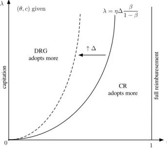
β λ
1 0
CR adopts more DRG
adopts more
↑∆ (θ, c) given
capitation
full reimburesement
λ=η∆ β 1−β
Figure 1: Optimal adoption: CR vs. heterogenous DRG.
to be treated with the new technology. Each of these additional patients generate
benefits (∆), and an operating marginal cost change of (1−β)(θ−c). We can
summarize this argument saying that the investment ofpmonetary units results in
a return of(η∆−(1−β)(θ−c))/(1−β). This corresponds to the denominator
of the right-hand fraction in (35).
We represent this comparison in Figure 1. The dividing line represents the
locus of(λ, β)values yielding the same marginal return of investment in the new
technology to the provider across regimes. The areas to the right and left of this line
indicate the parameter configurations yielding more technology adoption under the
payment scheme generating higher marginal net benefits to the provider.
Note that as the new technology embodies higher patients’ benefits compared
to the old one, the constellation of(λ, β)-values for which providers are willing
to adopt under cost reimbursement increases. This is a direct consequence of the
retrospective character of the cost reimbursement scheme. However, no clear-cut
comparison on the level of reimbursement along the indifference line can be
ob-tained. This is because such comparison involves comparing the values ofK2, α,
A similar argument can be put forward to analyze expression (36). The net
gains to the provider of an additional unit of the new technology under a
homoge-nous DRG reimbursement scheme areη∆−(θ−c). This is the denominator of the
left-hand fraction in (36). Under cost reimbursement, the investment ofpmonetary
units results in a return of(1/1−β)(η∆−(1−β)(θ−c)). This corresponds to
the denominator of the right-hand fraction in (36). The return of the investment is
thus larger under cost reimbursement, yielding the higher level of adoption.
7
Welfare analysis
So far we have identified the levels of technology adoption under different
reim-bursement rules and we have compared them as well, under some particular
con-ditions. To complete the analysis we need to assess whether these payment rules
induce over-adoption or under-adoption with respect to the first-best associated
with the social welfare.
For our purpose, we define the social welfare, in line with Levaggiet al.(2012)
and the literature in general, as the difference between benefits and costs. To obtain
explicit solutions and compare them with the corresponding adoption levels in (31),
(32) and (33), we shall assume again risk neutrality and a uniform distribution and
also normalizeq∗= 1. Then,
SW(¯q) =
Z q¯
0
bqf(q)dq+
Z q∗
¯
q
(q−q¯)ˆb+ ¯qbf(q)dq−
Z q¯
0
(pq¯+θq)f(q)dq−
Z q∗
¯
q
(pq¯+θq¯+c(q−q¯))f(q)dq−ξE(Rj) (37)
whereξrepresents the social cost of public funds `a la Laffont and Tirole (1986)10
andE(Rj)denote expected revenues under reimbursement rulej.
The expected revenues under the different reimbursements rules are given by
E(Rcr) =α+βhZ
¯
q
0
(pq¯+θq)f(q)dq+
Z q∗
¯
q
(pq¯+θq¯+c(q−q¯))f(q)dqi
(38)
E(Rhom) =
Z q∗
0
Kqf(q)dq=KE(q) (39)
E(Rhet) =
Z ¯q
0
K1qf(q)dq+
Z q∗
¯
q
(K1q¯+K2(q−q¯))f(q)dq (40)
7.1 Cost reimbursement rule
After substituting (38) into (37) we compute the first order condition:
∂SW
∂q¯ = (∆−(p+θ−c))(1−q¯)−pq¯−ξβ(p+ (θ−c)(1−q)) = 0.
Solving forq¯we obtain,
¯
qswcr= 1− p(1 +ξβ)
∆−(1 +ξβ)(θ−c). (41)
This is the welfare maximizing level of adoption under the cost reimbursement
rule. We want to compare this level of adoptionq¯swcrwith the corresponding level
of adoption that maximizes provider’s utility, namelyq¯cr.
A direct comparison of (31) and (41) yields
¯
qcr−q¯swcr= p(1 +ξβ)
∆−(1 +ξβ)(θ−c)−
p(1−β)
η∆−(1−β)(θ−c) >0.
Accordingly, under cost reimbursement the providerover-adoptsthe new
technol-ogy with respect to a welfare maximizing policy. The intuition behind the result
comes from the fact that the provider does not bear the full cost of the adoption.
7.2 Homogeneous DRG reimbursement rule
Substituting (39) into (37) we compute the first order condition,
∂SW
∂q¯ = (∆−(p+θ−c))(1−q¯)−pq¯= 0.
Solving forq¯we obtain,
¯
qswhom = 1− p
Now, comparing (32) and (42) we obtain
¯
qhom−q¯swhom = p
∆−(θ−c) −
p
η∆−(θ−c) ≥0.
That is forη > 1, the providerover-adoptsthe new technology because patients
are reimbursed at the same rate but patients’ benefits are larger under the new
technology. However, whenη = 1, the level of adoption is optimal. This is so
because given that both technologies are reimbursed at the same price,K, such
price is irrelevant in the adoption decision. Recall, that η = 1 means that the
semi-altruistic provider weights equally patients’ benefits and its financial results.
7.3 Heterogeneous DRG reimbursement rule
Substituting (40) into (37) we compute the first order condition,
∂SW
∂q¯ = (∆−(p+θ−c))(1−q¯)−pq¯−ξλ(1−q¯) = 0
Solving forq¯we obtain,
¯
qswhet = 1− p
∆−(θ−c)−ξλ (43)
A direct comparison of (33) and (43) yields
¯
qhet−q¯swhet= p
∆−(θ−c)−ξλ −
p
η∆−(θ−c) +λ >0.
Again, as under cost reimbursement, the providerover-adoptsthe new technology.
The intuition now relies in the fact that the new technology has a higher
reimburse-ment thus providing the incentives to over-invest in the new technology.
Note that the same (qualitative) results are obtained if we do not consider the
social cost of public funds (ξ= 0) following the approach `a la Baron and Myerson
(1982).
8
Final remarks
Adoption of new technologies is usually considered a main driver of growth of
health care costs.11 Many discussions about it exist. Arguments in favor of
cost-benefit analysis (health technology assessment) before the introduction of new
technologies has made its way into policy. We now observe in many countries
the requirement of an “economic test” before payment for new technologies is
ac-cepted by third-party payers (either public or private). This is especially visible
in the case of new pharmaceutical products and it has a growing trend in medical
devices.
However, there is a paucity of theoretical work related to the determinants of
adoption and diffusion of new technologies. We contribute toward filling this gap.
The novelty of our approach consists in allowing for an integrated treatment of
incentives for adoption of new technology under demand uncertainty. We identify
conditions for adoption under two different payment systems. Also, we compare
technology adoption across reimbursement systems in a simplified set-up. We now
summarize the main results.
Under a cost reimbursement system, large enough patient benefits are required
for adoption to occur. As long as patient benefits are above a certain threshold,
adoption of the new technology always occurs at strictly positive levels. However,
it is never optimal to expand the level of adoption to cover all demand (full
adop-tion). The threshold is given, in the case of risk neutrality and uniform distribution
for patient benefits, by the cost of treating a patient under the new technology
ac-counting for the savings resulting from not treating him under the old technology.
The cost reimbursement allows for the extreme cases of full cost reimbursement
and capitation (a fixed fee is paid, regardless of actual costs).
The other payment system we considered was prospective payments on a
sick-ness episode basis (the DRG system). Two different regimes can be envisaged
regarding the impact of using a new technology in the payment received by the
provider. In the first one, the treatment performed with the new technology is
clas-sified into the same DRG (and payment made by the third-party payer) as the old
technology. The second possibility is that the new technology leads to a payment
in a different DRG. When the DRG is not adjusted by the use of a new
technol-ogy, patients’ benefits are necessary to induce adoption. Whenever the DRG for