Open Some classical inequalities, summability of multilinear operators and strange functions

Gustavo da Silva Ara´

ujo

Some classical inequalities, summability of

multilinear operators and strange functions

Jo˜ao Pessoa-PB 2016

Universidade Federal da Para´ıba

Universidade Federal de Campina Grande

Programa Associado de P´os-Gradua¸c˜ao em Matem´atica

Doutorado em Matem´atica

Gustavo da Silva Ara´

ujo

Some classical inequalities, summability of

multilinear operators and strange functions

Tese apresentada ao Corpo Docente do Programa Associado de P´os-Gradua¸c˜ao em Matem´atica - UFPB/UFCG, como requisito parcial para a obten¸c˜ao do t´ıtulo de Doutor em Matem´atica.

Este exemplar corresponde a vers˜ao final da tese defendida pelo aluno Gustavo da Silva Ara´ujo e aprovada pela comiss˜ao julgadora.

Daniel Marinho Pellegrino (Orientador)

Maria Pilar Rueda Segado (Coorientadora)

Juan Benigno Seoane Sep´ulveda (Coorientador)

A663s Araújo, Gustavo da Silva.

Some classical inequalities, summability of multilinear operators and strange functions / Gustavo da Silva Araújo.- João Pessoa, 2016.

119f. : il.

Orientador: Daniel Marinho Pellegrino

Coorientadores: Maria Pilar Rueda Segado, Juan Benigno Seoane Sepúlveda

Tese (Doutorado) - UFPB-UFCG

1. Matemática.2. Desigualdade de Bohnenblust-Hille. 3. Desigualdade de Hardy-Littlewood. 4. Função contínua. 5. Função diferenciável. 6. Função mensurável. 7. Lineabilidade.

Universidade Federal da Para´ıba

Universidade Federal de Campina Grande

Programa Associado de P´os-Gradua¸c˜ao em Matem´atica

Doutorado em Matem´atica

Tese apresentada ao Corpo Docente do Programa Associado de P´os-Gradua¸c˜ao em Matem´atica - UFPB/UFCG, como requisito parcial para a obten¸c˜ao do t´ıtulo de Doutor em Matem´atica.

´

Area de Concentra¸c˜ao: An´alise

Aprovada em: 08 de mar¸co de 2016

Prof. Dr. Daniel Marinho Pellegrino Orientador

Universidade Federal da Para´ıba

Prof. Dr. Edgard Almeida Pimentel

Universidade Federal de S˜ao Carlos

Prof. Dr. Eduardo Vasconcelos Oliveira Teixeira

Universidade Federal do Cear´a

Prof. Dr. Jamilson Ramos Campos

Universidade Federal da Para´ıba

Prof. Dr. Nacib Andr´e Gurgel e Albuquerque

Universidade Federal da Para´ıba

Agradecimentos

Agrade¸co,

Aos meus amados pais, Maur´ıcio Ferreira de Ara´ujo e Elisa Clara Marques da Silva, respons´aveis pela educa¸c˜ao que tive, por me fazerem ter orgulho de onde vim, por terem me ensinado os valores que carrego at´e hoje e que hei de carregar durante toda a vida.

Aos meus irm˜aos, Maur´ıcio Ferreira de Ara´ujo Filho, Guilherme Maur´ıcio da Silva e Leonardo Ben´ıcio da Silva, pelo amor e compreens˜ao despendidos ao longo da vida.

A Pammella Queiroz de Souza, pela paciˆencia, ajuda e companheirismo nas horas de dedica¸c˜ao aos estudos e pelo amor que faz inundar nossas vidas.

Ao Prof. Daniel Marinho Pellegrino, amigo e orientador, pelos conselhos para a vida e, principalmente, por toda a colabora¸c˜ao e paciˆencia na elabora¸c˜ao deste trabalho.

Al Prof. Juan Benigno Seoane Sep´ulveda, por apoyarme en toda mi trayectoria cient´ıfica y personal en Madrid y por valiosas aportaciones y sugerencias para mi tra-bajo.

A profa. Maria Pilar Rueda Segado, sus generosas aportaciones han sido de funda-mental importancia.

Aos professores Edgard Almeida Pimentel, Eduardo Vasconcelos Oliveira Teixeira, Jamilson Ramos Campos e Nacib Andr´e Gurgel e Albuquerque, membros da banca exa-minadora, pela cuidadosa leitura e, principalmente, pelas valiosas corre¸c˜oes e sugest˜oes que ajudaram a melhorar o conte´udo final deste trabalho.

Al Prof. Gustavo Adolfo Mu˜noz Fern´andez, sin su apoyo no hubiera sido posible llevar acabo parte de esta investigaci´on.

Al prof. Luis Bernal Gonz´alez, su conocimiento, dedicaci´on y pasi´on por la ciencia me han inspirado en los momentos finales de este trabajo.

A todos aqueles que foram meus professores, n˜ao somente do ensino superior, vocˆes s˜ao verdadeiros her´ois; em especial, agrade¸co ao Prof. Uberlandio Batista Severo, meu orientador na gradua¸c˜ao e no mestrado, que teve fundamental importˆancia na minha forma¸c˜ao como matem´atico.

L´ısley Ramos Ara´ujo.

Gracias a toda la gente de la Universidad Complutense de Madrid, que me ha ayudado de una o otra forma; gracias Luis Fernando Echeverri Delgado, Maria Crespo Moya y Marcos Molina Rodr´ıguez, por estar siempre ah´ı haciendo m´as f´aciles las cosas.

To Suyash Pandey for his friendship in Madrid and for his kind comments and sug-gestions regarding this thesis.

A CAPES, pelo apoio financeiro.

Sucesso e vida longa a todos.

He explained it to me. He thought he had discovered a replacement for the equation.

Resumo

Este trabalho est´a dividido em trˆes partes. Na primeira parte, investigamos o comportamento das constantes das desigualdades polinomial e multilinear de Bohnenblust–Hille e Hardy–Littlewood. Na segunda parte, mostramos um resultado ´otimo de espa¸cabilidade para o complementar de uma classe de ope-radores m´ultiplo somantes em `p e tamb´em generalizamos um resultado

rela-cionado a cotipo (de 2010) devido a G. Botelho, C. Michels e D. Pellegrino. Al´em disso, provamos novos resultados de coincidˆencia para as classes de operadores multilineares absolutamente e m´ultiplo somantes (em particular, mostramos que o famoso teorema de Defant–Voigt ´e ´otimo). Ainda na se-gunda parte, mostramos uma generaliza¸c˜ao das desigualdades multilineares de Bohnenblust–Hille e Hardy–Littlewood e apresentamos uma nova classe de operadores multilineares somantes, a qual recupera as classes dos operadores multilineares absolutamente e m´ultiplo somantes. Na terceira parte, prova-mos a existˆencia de grandes estruturas alg´ebricas dentro de certos conjuntos, como, por exemplo, a fam´ılia das fun¸c˜oes mensur´aveis `a Lebesgue que s˜ao sobrejetivas em um sentido forte, a fam´ılia das fun¸c˜oes reais n˜ao constantes e diferenci´aveis que se anulam em um conjunto denso e a fam´ılia das fun¸c˜oes reais n˜ao cont´ınuas e separadamente cont´ınuas.

Palavras-chave: Desigualdade de Bohnenblust–Hille, desigualdade de Hardy–Littlewood, fun¸c˜ao cont´ınua, fun¸c˜ao diferenci´avel, fun¸c˜ao mensur´avel, lineabilidade, operadores mul-tilineares somantes.

Abstract

This work is divided into three parts. In the first part, we investigate the be-havior of the constants of the Bohnenblust–Hille and Hardy–Littlewood poly-nomial and multilinear inequalities. In the second part, we show an optimal spaceability result for a set of non-multiple summing forms on `p and we also

generalize a result related to cotype (from 2010) as highlighted by G. Botelho, C. Michels, and D. Pellegrino. Moreover, we prove new coincidence results for the class of absolutely and multiple summing multilinear operators (in par-ticular, we show that the well-known Defant–Voigt theorem is optimal). Still in the second part, we show a generalization of the Bohnenblust–Hille and Hardy–Littlewood multilinear inequalities and we present a new class of sum-ming multilinear operators, which recovers the class of absolutely and multiple summing operators. In the third part, it is proved the existence of large al-gebraic structures inside, among others, the family of Lebesgue measurable functions that are surjective in a strong sense, the family of non-constant di↵erentiable real functions vanishing on dense sets, and the family of non-continuous separately non-continuous real functions.

Key-words: Bohnenblust–Hille inequality, continuous function, di↵erentiable function, Hardy–Littlewood inequality, lineability, measurable function, summing multilinear ope-rators.

Contents

Introduction 1

Preliminaries and Notation 7

I

The Bohnenblust–Hille and Hardy–Littlewood inequalities 13

1 The m-linear Bohnenblust–Hille and Hardy–Littlewood inequalities 15

1.1 Lower and upper bounds for the constants of the classical Hardy–Littlewood

inequality . . . 20

1.2 On the constants of the generalized Bohnenblust–Hille and Hardy–Littlewood inequalities . . . 27

1.2.1 Estimates for the constants of the generalized Bohnenblust–Hille inequality . . . 28

1.2.2 Application 1: Improving the constants of the Hardy–Littlewood inequality . . . 31

1.2.3 Application 2: Estimates for the constants of the generalized Hardy– Littlewood inequality . . . 33

2 Optimal Hardy–Littlewood type inequalities for m-linear forms on `p spaces with 1 _ p_ m 37 3 On the polynomial Bohnenblust–Hille and Hardy–Littlewood inequali-ties 43 3.1 Lower bounds for the complex polynomial Hardy–Littlewood inequality . . 45

3.2 The complex polynomial Hardy–Littlewood inequality: Upper estimates . . 48

II

Summability of multilinear operators

51

4.2 Some consequences . . . 58

4.3 Multiple (r;s)-summing forms in c0 and `1 spaces . . . 61

5 A unified theory and consequences 67

5.1 Multiple summing operators with multiple exponents . . . 67 5.2 Partially multiple summing operators: The unifying concept . . . 76

III

Strange functions

85

6 Lineability in function spaces 87

6.1 Measurable functions . . . 87 6.2 Special di↵erentiable functions . . . 89 6.3 Discontinuous functions . . . 91

References 93

Introduction

Part I: The Bohnenblust–Hille and Hardy–Littlewood

inequalities

To solve a problem posed by P.J. Daniell, Littlewood [101] proved in 1930 his famous 4/3-inequality, which asserts that

1 P

i,j=1|

T(ei, ej)|

4 3

!3 4

p2_kT_k,

for every continuous bilinear form T : c0 ⇥ c0 ! K. One year later, and due to his

interest in solving a long standing problem on Dirichlet series, H.F. Bohnenblust and E. Hille proved in [42] a generalization of Littlewood’s 4/3 inequality to m-linear forms: there exists a (optimal) constant Bmult

K,m ≥ 1 such that for all continuous m-linear forms

T : `n

1 ⇥ · · · ⇥`n1 ! K and all positive integers n,

n

P

j1,...,jm=1

|T(ej1, ..., ejm)| 2m m+1

!m+1 2m

 Bmult

K,m kTk.

The problem was posed by H. Bohr and consisted in determining the width of the maxi-mal strips on which a Dirichlet series can converge absolutely but non uniformly. More precisely, for a Dirichlet series P_nann−s, Bohr defined

σ_a = inf

⇢ r :P

n

a_nn−s _{converges for Re(s)> r}

% ,

σu = inf

⇢ r : P

n

ann−s converges uniformly in Re(s) > r+" for every " >0

%

and S := sup_{σ_a−σ_u}. Bohr’s question asked for the precise value of S. The answer came from H.F. Bohnenblust and E. Hille (1931): S = 1/2. The main tool is the, by now, so-called Bohnenblust–Hille inequality. The precise growth of the constants Bmult

K,m

is important for applications and is nowadays a challenging problem in Mathematical Analysis. For real scalars, the estimates of Bmult

R,m are important in Quantum Information

2

inequality have been published and several advances were achieved (see [6, 62, 65, 68, 111, 119, 129] and the references therein). Only very recently, in [32, 111] it was shown that the constants Bmult

K,m have a sublinear growth, which means a major change in this

panorama since all previous estimates (from 1931 up to 2011) predicted an exponential growth. For real scalars, in 2014 (see [75]) it was shown that the optimal constant for

m = 2 is p2 and in general Bmult

R,m ≥ 21−

1

m. In the case of complex scalars it is still an

open problem whether the optimal constants are strictly greater than 1.

Given↵= (↵1, . . . , ↵n) 2Nn, define|↵|:= ↵1+· · ·+↵nandx↵ stands for the monomial

x↵1

1 · · ·x↵nn, for x = (x1, . . . , xn) 2Kn. The polynomial Bohnenblust–Hille inequality (see

[6, 42] and the references therein) ensures that, given positive integersm _≥2 andn _≥1, if

P is a homogeneous polynomial of degree m on `n

1 given by P(x1, ..., xn) = P_|↵|=ma↵x↵,

then

P |↵|=m|

a↵|

2m m+1

!m+1 2m

B_Kpol_,mkP_k,

for some constant B_Kpol_{,m ≥} 1 which does not depend on n (the exponent _m2₊₁m is optimal), where _kP_k := sup_z2B`n

1 |P(z)|. The search of precise estimates of the growth of the constantsB_Kpol_,m is crucial for di↵erent applications and remains an important open problem (see [32] and the references therein). For real scalars, it was shown in [56] that the hypercontractivity of B_Rpol_,m is optimal. For complex scalars the behavior of B_Kpol_,m is still unknown. Moreover, in the complex scalar case, having good estimates for B_Cpol_,m is crucial to applications in Complex Analysis and Analytic Number Theory (see [65]); for instance, the subexponentiality of the constants of the polynomial version of the Bohnenblust–Hille inequality (complex scalars case) was recenly used in [32] in order to obtain the asymptotic growth of the Bohr radius of the n-dimensional polydisk. More precisely, according to Boas and Khavinson [41], the Bohr radiusKn of the n-dimensional polydisk is the largest

positive number r such that all polynomials P_↵a_↵z↵ _{on C}n _satisfy

sup

z2rDn

P

↵ |

a↵z↵|  sup z2Dn

& & &

&P_↵ a↵z↵

& & & &.

The Bohr radius K₁ was estimated by H. Bohr, and it was later shown (independently) by M. Riesz, I. Schur and F. Wiener that K1 = 1/3 (see [41, 43] and the references

therein). For n _≥ 2, exact values of Kn are unknown. In [32], the subexponentiality of

the constants of the complex polynomial version of the Bohnenblust–Hille inequality was established and using this fact it was finally proved that

lim

n!1

Kn plogn

n

= 1,

solving a challenging problem in Mathematical Analysis.

The Hardy-Littlewood inequality is a natural generalization of the Bohnenblust–Hille inequality for `p spaces. The bilinear case was proved by Hardy and Littlewood in 1934

(see [91]) and in 1981 it was extended to multilinear operators by Praciano-Pereira (see [128]). More precisely, the classical Hardy–Littlewood inequality asserts that for 0 _

3

for all positive integers n and all continuous m-linear forms T :`n

p1 ⇥ · · · ⇥`

n

pm ! K,

n

P

j1,...,jm=1

|T(e_j1, ..., e_jm)_|

2m m+1−2|1

p|

!m+1−2|_p1| 2m

Cmult

K,m,pkTk.

When _|1/p_| = 0 (or equivalently p₁ = _{· · ·} = p_m = ₁) since 2m/(m + 1₋ 2_|1/p_|) = 2m/(m+ 1), we recover the classical Bohnenblust–Hille inequality (see [42]).

When replacing`n

1 by`np the extension of the polynomial Bohnenblust–Hille inequality

is called polynomial Hardy–Littlewood inequality. More precisely, given positive integers

m_≥ 2 andn _≥1, ifP is a homogeneous polynomial of degreemon`n

p, with 2mp  1,

given by P(x1, . . . , xn) = P_|↵|=ma↵x↵, then there is a constant CKpol,m,p ≥ 1 such that

P |↵|=m

|a↵|

2mp mp+p−2m

!mp+p−2m 2mp

 C_Kpol_,m,pkP_k,

and C_Kpol_,m,p does not depend on n, where _kP_k := sup_z2B

`np |P(z)|.

When p = ₁ we recover the polynomial Bohnenblust–Hille inequality. Using the generalized Kahane–Salem–Zygmund inequality (see, for instance, [6]) we can verify that the exponents in the above inequalities are optimal. The precise estimates of the constants of the Hardy–Littlewood inequalities are unknown and even its asymptotic growth is a mystery (as it happens with the Bohnenblust–Hille inequality).

Very recently, an extended version of the Hardy–Littlewood inequality was presented in [6] (see also [73]).

Theorem 0.1 (Generalized Hardy–Littlewood inequality for 0 _{ |}1/p_{| } 1/2). Let p := (p₁, . . . , p_m) ₂ [1,+₁]m _{such that 0  |1/p|  1/2. Let also q := (q}

1, . . . , qm) 2 [(1 −

|1/p_|)−1_,2]m_{. The following are equivalent:}

(1) There is a (optimal) constant C_Kmult_{,m,p,q ≥}1 such that

0 B @P1

j1=1

0

@_{· · ·} P1

jm=1

|T (ej1, . . . , ejm)|

qm

!qm−1 qm

· · ·

1 A

q₁ q₂1

C A

1 q₁

 C_Kmult_,m,p,qkT_k

for all continuous m-linear forms T :Xp1 ⇥ · · · ⇥Xpm ! K.

(2) _q1

1 +· · ·+

1

qm 

m+1

2 −

& & &p1

& & &.

For the case 1/2_{ |}1/p_| <1 there is also a version of the multilinear Hardy–Littlewood inequality, which is an immediate consequence of Theorem 1.2 from [5] (see also [73]).

Theorem 0.2 (Hardy–Littlewood inequality for 1/2 _{ |}1/p_| < 1). Let m _≥ 1 and

p = (p1, . . . , pm) 2 [1,1]m be such that 1/2  |1/p| < 1. Then there is a (optimal)

constant Dmult_{K,m,p ≥} 1 such that

N

P

i1,...,im=1

|T(ei1, . . . , eim)| 1 1−|_p1|

!1−|p1|

 Dmult

4

for every continuous m-linear operator T : `N

p1 ⇥ · · · ⇥`

N

pm ! K. Moreover, the exponent

(1_{− |}1/p_|)−1 _{is optimal.}

In this part of the work, we investigate the behavior of the constants Cmult

K,m,p,q, DmultK,m,p

(Chapter 1) andC_Kpol_,m,p (Chapter 3). In Chapter 2 we answer, for 1 _ p_ m, the question on how the Hardy–Littlewood multilinear inequalities behave if we replace the exponents 2mp/(mp+p₋ 2m) and p/(p₋ m) by a smaller value r (see Theorem 2.1). This case (1 _ p _ m) was only explored for the case of Hilbert spaces (p = 2, see [47, Corollary 5.20] and [61]) and the case p =₁ was explored in [57].

Part II: Summability of multilinear operators

In 1950 A. Dvoretzky and C. A. Rogers [76] solved a long standing problem in Banach Space Theory when they proved that in every infinite-dimensional Banach space there exists an unconditionally convergent series which is not absolutely convergent. This result is the answer to Problem 122 of the Scottish Book [104], addressed by S. Banach in [26, page 40]). It was the starting point of the theory of absolutely summing operators.

A. Grothendieck, in [88], presented a di↵erent proof of the Dvoretzky-Rogers theorem and his “R´esum´e de la th´eorie m´etrique des produits tensoriels topologiques” brought many illuminating insights to the theory of absolutely summing operators.

The notion of absolutelyp-summing linear operators is credited to A. Pietsch [124] and the notion of (q, p)-summing operator is credited to B. Mitiagin and A. Pe lczy´nski [105]. In 1968 J. Lindenstrauss and A. Pe lczy´nski’s seminal paper [100] re-wrote Grothendieck’s R´esum´e in a more comprehensive form, putting the subject in the spotlight. In 2003 M. Matos [102] and, independently, F. Bombal, D. P´erez-Garc´ıa and I. Villanueva [44] intro-duced a more general notion of absolutely summing operators called multiple summing multilinear operators, which has gained special attention, being considered by several au-thors as the most important multilinear generalization of absolutely summing operators: let 1 _ p1, . . . , pm  q < 1. A bounded m-linear operator T : E1 ⇥ · · · ⇥Em ! F is

multiple (q;p1, . . . , pm)-summing if there exists Cm > 0 such that

1 P

j1,...,jm=1

--T(x(1)_j1 , . . . , x_j(_mm))--_-q

!1 q

 Cm m

Q

k=1

--(x(_jk))1_j=1--

-w,pk

,

for every (x(_jk))1

j=1 2 `wpk(Ek), k = 1, . . . , m. The class of all multiple (q;p1, . . . , pm

)-summing operators from E1 ⇥ · · · ⇥Em to F will be denoted by

⇧m_{mult(q;p1,...,pm)}(E1, . . . , Em;F).

The roots of the subject could probably be traced back to 1930, when, as we have already said, Littlewood [101] proved his famous 4/3-inequality to solve a problem posed by P.J. Daniell. One year later, interested in solving a long standing problem on Dirichlet series, H.F. Bohnenblust and E. Hille generalized Littlewood’s 4/3 inequality to m -linear forms. Using that _L(c0;E) is isometrically isomorphic to `w1 (E) (see [72]), the

5

inequality [42] ensures that, for all m_≥ 2 and all Banach spaces E1, ..., Em,

L(E₁, ..., E_m;K) = ⇧m

mult(_m+12m ;1,...,1) (E1, ..., Em;K).

In Chapter 4 we prove that, if 1 < s < p⇤_{, the set (L(}m_`

p;K)r⇧m_mult( 2m m+1;s)

(m_`

p;K))[

{0_} contains a closed infinite-dimensional Banach space with the same dimension of

L(m_`

p;K). As a consequence we observe, for instance, a new optimal component of

the Bohnenblust–Hille inequality: the terms 1 from the tuple (2m/(m + 1); 1, ...,1) is also optimal. Moreover, we generalize a result related to cotype (from 2010) due to G. Botelho, C. Michels, and D. Pellegrino, and we investigate the optimality of coincidence results for multiple summing operators in c0 and in the framework of absolutely summing

multilinear operators. As a result, we observe that the Defant–Voigt theorem is optimal. In Chapter 5 we present a new class of summing multilinear operators, which recovers the class of absolutely (and multiple) summing operators. Moreover, we present a unified version of the Bohnenblust–Hille and the Hardy–Littlewood inequalities with partial sums which ensures that these results are in fact, corollaries of a unique yet general result.

Part III: Strange functions

Lebesgue ([99], 1904) was probably the first to show an example of a real function on the reals satisfying the rather surprising property that it takes on each real value in any nonempty open set (see also [86, 87]). The functions satisfying this property are called everywhere surjective (functions with even more stringent properties can be found in [80, 95]). Of course, such functions are nowhere continuous but, as we will see later, it is possible to construct a Lebesgue measurable everywhere surjective function. Entering a very di↵erent realm, in 1906 Pompeiu [126] was able to construct a nonconstant di↵erentiable function on the reals whose derivative vanishes on a dense set. Passing to several variables, the first problem one meets related to the “minimal regularity” of functions at a elementary level is that of whether separate continuity implies continuity, the answer being given in the negative.

In this part of the thesis we will consider the families consisting of each of these kinds of functions and analyze the existence of large algebraic structures inside all these families. Nowadays the topic of lineability has had a major influence in many di↵erent areas on mathematics, from Real and Complex Analysis [29], to Set Theory [84], Operator Theory [92], and even (more recently) in Probability Theory [79]. Our main goal here is to continue with this ongoing research. We will focus on diverse lineability properties of the families _MES (the family of Lebesgue measurable functions R _! R that are everywhere surjective), _P (the vector space of Pompeiu functions, i.e., the functions f : R _! R that are di↵erentiable and f0 _{vanishes on a dense set in R), DP (the vector space}

Preliminaries and Notation

For any function f, whenever it makes sense, we formally define f(₁) = limp!1f(p).

Throughout this thesis, E, E1, E2, . . . , F shall denote Banach spaces over K, which shall

stands for the complex C or real R fields. In addition, _L(E1, ..., Em;F) stands for the

Banach space of all bounded m-linear operators from E_{1 ⇥ · · · ⇥} E_m to F under the supremum norm and when E1 =· · · =Em = E we denote L(E1, ..., Em;F) by L(mE;F).

The topological dual of E shall be denoted by E⇤ _{and for any p ≥ 1 its conjugate is}

represented by p⇤, i.e., 1/p+ 1/p⇤ = 1. For p ₂ [1,₁], as usual, we consider the Banach spaces of weakly and strongly p-summable sequences, respectively, as bellow:

`w_p(E) :=

8 <

:(xj)1j=1 ⇢ E :

--(xj)1j=1

-w,p := sup '2BE⇤

1 P

j=1|

'(xj)|p

!1/p

< ₁ 9 = ;

and

`_p(E) :=

8 <

:(xj)1j=1 ⇢ E : --(x_j)1

j=1

-p :=

1 P

j=1k

x_jkp !1/p

<₁ 9 = ;

(naturally, the sum P should be replaced by the supremum if p = ₁). Besides, we set

X₁ := c0 and Xp := `p := `p(K). For a positive integer m, p stands for a multiple

exponent (p1, . . . , pm) 2[1,1]m and

& & &p1

& & &:= _p1

1 +· · ·+

1

pm.

Khinchine’s inequality

The real Khinchine inequality (see [72]) asserts that for any 0 < q < ₁, there are positive constants AR,q, BR,q such that, regardless of the scalar sequence (aj)1j=1 in `2, we

have

AR,q

1 P

j=1|

aj|2

!1 2

 R01

& & & & &

1 P

j=1

ajrj(t)

& & & & &

q

dt !1

q

 BR,q

1 P

j=1|

aj|2

!1 2

,

where rj are the Rademacher functions. More generally, from the above inequality

refe-8

rences therein)

AmR,q

1 P

j1,...,jm=1

|aj1···jm|

2

!1 2

 R_I

& & & & &

1 P

j1,...,jm=1

aj1···jmrj1(t1)· · ·rjm(tm)

& & & & &

q

dt !1

q

 BRm,q

1 P

j1,...,jm=1

|aj1···jm|

2

!1 2

, (1)

where I = [0,1]m _{and dt = dt}

1· · ·dtm, for all scalar sequences (aj1···jm)

1

j1,...,jm=1 in `2.

The optimal constants AR,q of the Khinchine inequality (these constants are due to U.

Haagerup [90]) are:

• AR,q =

p

2

✓

Γ(1+q₂ )

p_⇡ ◆1

q

if q > q0 ⇠= 1.8474;

• AR,q = 2

1 2−

1

q if q < q

0.

The definition of the number q0 above is the following: q0 2 (1,2) is the unique real

number with

Γ8q0+1

2

9

= p₂⇡.

For complex scalars, using Steinhaus variables instead of Rademacher functions it is well known that a similar inequality holds, but with better constants (see [98, 133]). In this case the optimal constant is:

• AC,q = Γ

8_q+2

2

91 q _{if q}

2 [1,2].

The notation of the constant AK,q shown above will be employed throughout this thesis.

Kahane–Salem–Zygmund’s inequality

Using the argument introduced in [39, Theorem 4] we present a variant of a result by Boas, that first appeared in [6, Lemma 6.1], and that is proved in [1].

Kahane–Salem–Zygmund’s inequality. Let m, n _≥ 1, p₁, ..., p_{m 2} [1,+₁]m _{and, for}

p_≥ 1, define

↵(p) =

⇢ 1 2 −

1

p , if p ≥2;

0, otherwise.

Then there exists a m-linear map A :`n<sub>p1 ⇥ · · · ⇥</sub>`n_{pm !} K of the form

A(z1, . . . , zm) = n

P

j1,...,jm=1

✏j1...jmzj11· · ·z

d jm

with ✏j1···jm 2 {−1,1}, such that

kA_{k } Cm ·n

1

2+↵(p1)+···+↵(pm) (2)

where Cm = (m!)1−

1

9

The essence of the Kahane–Salem–Zygmund inequalities probably appeared for the first time in [96], but our approach follows the lines of Boas’ paper [39]. Paraphrasing Boas, the Kahane–Salem–Zygmund inequalities use probabilistic methods to construct a homogeneous polynomial (or multilinear operator) with a relatively small supremum norm but relatively large majorant function (we refer [1, Appendix B] for a more detailed study of the Kahane–Salem–Zygmund inequalities).

Minkowski’s inequality

The following result is a corollary of one of the many versions of Minkowski’s inequality, whose proof can be found, for instance, in [85, Corollary 5.4.2].

Minkowski’s inequality. For any 0 < p _q < 1 and for any scalar matrix (aij)i,j2N,

0 @P1

i=1

1 P

j=1|

aij|p

!q p1

A

1 q

 P1

j=1

✓₁ P

i=1|

aij|q

◆p q!

1 p

.

H¨

older’s (interpolative) inequality for mixed

`

spaces

The following general H¨older’s inequality was presented in the classical paper [33] on mixed norms in Lp spaces. We shall now work with Lp(N) = `p, since it is the case we are

interested in. We need to recall some useful multi-index notation: for a positive integer

m and a non-void subset D _⇢ N we denote the set of multi-indices i = (i1, . . . , im), with

each i_{k 2}D, by

M(m, D) :=_{i = (i1, . . . , im)2 Nm; ik 2D, k = 1, . . . , m} =Dm.

We also denote

M(m, n) := _M(m,_{1,2, . . . , n_}).

For p = (p₁, . . . , p_m) ₂[1,₁)m_{, and a Banach space E, let us consider the space}

`p(X) :=`p1(`p2(. . .(`pm(X)). . .)),

namely, a vector matrix (xi)_i2M(m,N) 2 `p(X) if, and only if,

0 B B @

1 P

i1=1

0 B @P1

i2=1

0

@. . . P1

im−1=1

✓ ₁ P

im=1

kxikp_Em

◆pm−1 pm !

pm−2 pm−1

. . . 1 A

p₂ p₃1

C A

p₁ p₂1

C C A

1 p₁

<₁.

When X = K, we just write `p instead of `p(K). Also, we deal with the coordinatewise

product of two scalar matrices a = (ai)_i2M(m,n) and b= (bi)_i2M(m,n), i.e.,

ab := (aibi)_i2M(m,n).

10

[33]):

H¨older’s inequality for mixed `p spaces. Let m, n, N be positive integers, r 2 [1,1)m

and q(1), . . . ,q(N) ₂[1,₁]m _{be such that}

1

rj =

1

qj(1) +· · ·+

1

qj(N), j 2 {1,2, . . . , m}

and also let ak := (aki)i_2M(m,n), k = 1, . . . , N be scalar matrices. Then

-N Q k=1 a_k -r

 QN

k=1k

a_kkq(k).

In particular, if each q(k) ₂[1,₁)m_{, we have}

0 @Pn

i1=1

. . . ✓ _n

P

im=1 |a1

ia2i . . . aNi |qm

◆qm−1 qm

. . . !q₁

q₂1

A

1 q₁

 QN

k=1 2 6 6 4 0 B @ n P

i1=1

0 @. . .

✓ _n P

im=1

|ak_i|qm(k)

◆qm−1(k) qm(k)

. . . 1 A

q₁₍k) q₂₍k)1

C A

1 q₁₍k)3

7 7 5.

Using the above result we are able to recover the interpolative inequality from [5, 6, 7, 32] (see also [4]) that we can also, in some sense, call H¨older’s inequality for multiple exponents. Under the point of view of interpolation theory it is not a complicated result but, just in 2013, it began to be used in all its full strength.

For a positive real number ✓, let us define a✓ _:= 8_a✓

i

9

i_2M(m,n). It is straightforward to

see that

--a✓--_q/✓ =_ka_k✓_q,

where q/✓ := (q1/✓, . . . , qm/✓).

H¨older’s interpolative inequality for multiple exponents. Let m, n, N be positive integers andr,q(1), . . . ,q(N) ₂[1,₁]m _{and ✓}

1, . . . , ✓N 2[0,1]be such that ✓1+· · ·+✓N =

1 and

1

rj =

✓1

qj(1) +· · ·+

✓N

qj(N), for all j = 1, . . . , m.

Then, for all scalar matrix a = (ai)i_2M(m,n) we have

ka_{kr } QN

k=1k a_k✓k

q(k).

In particular, if each q(k) ₂[1,₁)m, the previous inequality means that

0 B @

n

X

i1=1

0 @. . .

n

X

im=1 |ai|rm

!rm−1 rm

. . . 1 A

r₁ r₂1

C A

11

 QN

k=1

2 6 6 4

0 B @

n

P

i1=1

0 @. . .

✓ _n P

im=1

|ai|qm(k)

◆qm−1(k) qm(k)

. . . 1 A

q₁₍k) q₂₍k)1

C A

1 q₁₍k)3

7 7 5

✓k

.

Lineability notions

A number of concepts have been coined in order to describe the algebraic size of a given set; see [21, 31, 35, 78, 89] (see also the survey paper [38] and the forthcoming book [18] for an account of lineability properties of specific subsets of vector spaces). Namely, if X is a vector space, ↵ is a cardinal number and A _⇢X, then A is said to be:

• lineable if there is an infinite dimensional vector space M such that M _{\ {}0_{} ⇢} A,

• ↵-lineable if there exists a vector space M with dim(M) = ↵ and M _{\ {}0_{} ⇢} A

(hence lineability means _@0-lineability, where @0 = card (N), the cardinality of N),

and

• maximal lineable in X if A is dim (X)-lineable.

If, in addition, X is a topological vector space, then A is said to be:

• dense-lineable in X whenever there is a dense vector subspace M of X satisfying

M _{\ {}0_{} ⇢} A (hence dense-lineability implies lineability as soon as dim(X) = ₁), and

• maximal dense-lineable in X whenever there is a dense vector subspace M of X

satisfying M _{\ {}0_{} ⇢}A and dim (M) = dim (X),

• spaceable in X if there is a closed infinite dimensional vector subspace M such that

M _{\ {}0_{} ⇢} A (hence spaceability implies lineability), and

• maximal spaceable in X if A in X is spaceable and dim(A) = dim(X).

According to [24, 28], when X is a topological vector space contained in some (linear) algebra, then A is called:

• algebrableif there is an algebra M so that M_\{0_{} ⇢} AandM is infinitely generated, that is, the cardinality of any system of generators of M is infinite.

• densely algebrable in X if, in addition, M can be taken dense in X.

• ↵-algebrable if there is an ↵-generated algebra M with M _{\ {}0_{} ⇢}A.

• strongly ↵-algebrableif there exists an↵-generatedfreealgebra M with M_\{0_{} ⇢} A

(for ↵= _@0, we simply say strongly algebrable).

• densely strongly ↵-algebrable if, in addition, the free algebra M can be taken dense in X.

Part I

Chapter

1

The

m

-linear Bohnenblust–Hille and

Hardy–Littlewood inequalities

In 1931 F. Bohnenblust and E. Hille proved in [42] that there exists a (optimal) constant B_Kmult_{,m ≥} 1 such that for all continuous m-linear forms T : `n<sub>1 ⇥ · · · ⇥</sub>`n_{1 !} K, and all positive integers n,

n

P

j1,...,jm=1

|T(ej1, ..., ejm)| 2m m+1

!m+1 2m

 Bmult

K,m kTk. (1.1)

The precise growth of the constantsBmult

K,m is important for many applications (see, e.g.,

[106]) and remains an open problem. Only very recently, in [32, 111] it was shown that the constants have a sublinear growth. For real scalars (2014, see [75]) it was shown that the optimal constant form = 2 isp2 and in general Bmult

R,m ≥ 21−

1

m. In the case of complex

scalars it is still an open problem whether the optimal constants are strictly grater than 1; in the polynomial case, in 2013 D. N´u˜nez-Alarc´on proved that the complex constants are strictly greater than 1 (see [108]). Even basic questions related to the constants B_Kmult_,m

remain unsolved. For instance:

• Is the sequence of optimal constants 8B_Kmult_,m91_m=1 increasing?

• Is the sequence of optimal constants 8Bmult

K,m

91

m=1 bounded?

• Is Bmult

C,m = 1?

The best known estimates for the constants in (1.1), which are recently presented in [32], are (Bmult

K,1 = 1 is obvious)

B_Kmult_{,m }

m

Q

j=2

A−_K1

,2j_j−2,

where AK,(2j−2)/j are the respective constants of the Khnichine inequality, i.e.,

B_Cmult_{,m } Qm

j=2

Γ⇣2₋ 1_j⌘

j 2−2j

16 Chapter 1. The m-linear Bohnenblust–Hille and Hardy–Littlewood inequalities

Bmult

R,m  m

Q

j=2

22j1−2, for 2 m13,

Bmult

R,m  2

446381 55440−

m 2

m

Q

j=14

✓

Γ(3₂−1j)

p

⇡

◆ j 2−2j

, for m_≥ 14.

(1.2)

In a more friendly presentation the above formulas tell us that the growth of the constants

Bmult

K,m is sublinear since, from the above estimates it can be proved that (see [32])

Bmult

C,m < m

1−γ

2 < m0.21139,

BRmult,m < 1.3·m

2−log 2−γ

2 <1.3·m0.36482,

where γ denotes the Euler–Mascheroni constant. Di↵erently of the above estimates, all previous estimates (from 1931 up to 2011) predicted an exponential growth. It was only in 2012, with [119] (motivated by [68]), when the perspective on the subject changed entirely.

The Hardy-Littlewood inequality is a natural generalization of the Bohnenblust–Hille inequality to `p spaces. More precisely, the classical Hardy–Littlewood inequality asserts

that for 0 _{ |}1/p_{| } 1/2 there exists a (optimal) constant Cmult

K,m,p ≥ 1 such that, for all

positive integers n and all continuous m-linear forms T :`n

p1 ⇥ · · · ⇥`

n

pm ! K,

n

P

j1,...,jm=1

|T(ej1, ..., ejm)| 2m m+1−2|_p1|

!m+1−2|1

p|

2m

 Cmult

K,m,pkTk. (1.3)

Using the generalized Kahane-Salem-Zygmund inequality (2) (see [6]) one can easily verify that the exponents 2m/(m+ 1₋ 2_|1/p_|) are optimal. When _|1/p_| = 0 (or equivalently

p1 = · · · = pm = 1), since 2m/(m+ 1−2|1/p|) = 2m/(m+ 1), we recover the classical

Bohnenblust–Hille inequality (see [42]).

The precise estimates of the constants of the Hardy–Littlewood inequalities are un-known and even its asymptotic growth is a mystery (as it happens with the Bohnenblust– Hille inequality). The original estimates for C_Kmult_,m,p (see [6]) were of the form

C_Kmult_{,m,p } 8p29m−1. (1.4) Very recently an extended version of the Hardy–Littlewood inequality was presented in [6] (see also [73]).

Theorem 1.1 (Generalized Hardy–Littlewood inequality for 0 _{ |}1/p_{| } 1/2). Let p:= (p1, . . . , pm) 2 [1,+1]m be such that 0  |1/p|  1/2. Let also q := (q1, . . . , qm) 2

[(1_{− |}1/p_|)−1_,2]m_{. The following are equivalent:}

(1) There is a (optimal) constant Cmult

K,m,p,q ≥ 1 such that

0 B @P1

j1=1

0

@_{· · ·} P1

jm=1

|T (ej1, . . . , ejm)|

qm

!qm−1 qm

· · ·

1 A

q₁ q₂1

C A

1 q₁

 Cmult

K,m,p,qkTk

17

(2) _q1

1 +· · ·+

1

qm 

m+1

2 −

& & &p1

& & &.

Some particular cases of C_Kmult_,m,p,q will be used throughout this chapter, therefore, we will establish notations for the (optimal) constants in some special cases:

• If p1 = · · · = pm = 1 we recover the generalized Bohnenblust–Hille

inequa-lity and we will denote Cmult

K,m,(1,...,1),q by BKmult,m,q. Moreover, if q1 = · · · = qm =

2m/(m+ 1) we recover the classical Bohnenblust–Hille inequality and we will de-note B_Kmult_{,m,(2m/(m+1),...,2m/(m+1))} by B_Kmult_,m;

• If q1 = · · · =qm = 2m/(m+ 1−2|1/p|) we recover the classical Hardy–Littlewood

inequality and we will denoteC_Kmult_{,m,p,(2m/(m+1−2|1/p|),...,2m/(m+1−2|1/p|))} byC_Kmult_,m,p. More-over, if p1 =· · · =pm =p we will denote CKmult,m,p by CKmult,m,p.

For the case 1/2_{ |}1/p_| <1 there is also a version of the multilinear Hardy–Littlewood inequality, which is an immediate consequence of Theorem 1.2 from [5] (see also [73]).

Theorem 1.2 (Hardy–Littlewood inequality for 1/2_{ |}1/p_| <1). Let p = (p₁, . . . , p_m)₂ [1,₁]m _{be such that 1/2  |1/p|< 1. Then there is a (optimal) constant D}mult

K,m,p ≥1 such

that

N

P

i1,...,im=1

|T(ei1, . . . , eim)| 1 1−|1

p|

!1−|p1|

 DKmult,m,pkTk

for every continuous m-linear operator T : `N<sub>p1 ⇥ · · · ⇥</sub>`N_{pm !} K. Moreover, the exponent (1_{− |}1/p_|)−1 _{is optimal.}

The best known upper bounds for the constants on the previous result are Dmult

R,m,p 

8p

29m−1 andDmultC,m,p  (2/

p

⇡)m−1 (see [5, 73]). We will only deal with this second case of the Hardy–Littlewood inequality in Chapters 2 and 5. Again, we will establish notations for the (optimal) constants Dmult

K,m,p in some special cases:

• When p1 =· · ·= pm =p we denote DmultK,m,p by DmultK,m,p.

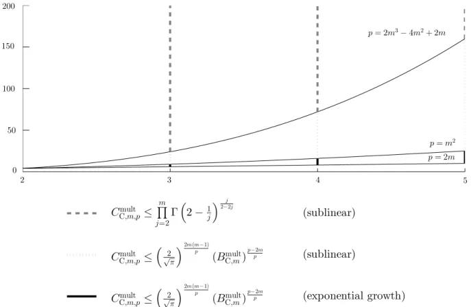
Our main contributions regarding the constants of the multilinear case of the Hardy– Littlewood inequality can be summarized in the following result, which is a direct conse-quence of the forthcomings sections 1.1 and 1.2.

Theorem 1.3. Let m_≥ 2 and let σR = p

2 and σC = 2/p⇡. Then,

(1) Let q = (q1, ..., qm) 2[1,2]m such that |1/q| = (m+ 1)/2 and maxqi < (2m2−4m+

2)/(m2 _{−m−1), then}

B_Kmult_{,m,q }

m

Q

j=2

A−_K1

,2j_j−2.

(2) Cmult

R,m,p ≥ 2

mp+2m−2m2−p

mp for 2m < p 1 and Cmult

18 Chapter 1. The m-linear Bohnenblust–Hille and Hardy–Littlewood inequalities

(3) (i) For _|1/p_{| } 1/2,

CKmult,m,p  (σK)

2(m−1)|1_p|8

BKmult,m

91−2|_p1|

.

In particular, 8Cmult

K,m,p

91

m=1 is sublinear if |1/p|  1/m.

(ii) For 2m3₋4m2 + 2m < p_{ 1},

Cmult

K,m,p  m

Q

j=2

A−_K1

,2j_j−2.

(4) Let 2m < p _{ 1} and let q := (q₁, ..., q_m) ₂ [p/(p ₋ m),2]m _{such that |1/q| =}

(mp+p₋2m)/2p. If maxqi <(2m2 −4m+ 2)/(m2 −m−1), then

Cmult

K,m,p,q 

m

Q

j=2

A−_K1

,2j_j−2.

Note that, for instance, if 2m3_−4m2_{+ 2m < p  1, the formula of item(3)(ii) is not}

dependent on p, contrary to what happens in item (3)(i), where we can see a dependence on p but, paradoxically, it is worse than the formula from item (3)(ii). This suggests the following problems:

• Are the optimal constants of the Bohnenblust–Hille and Hardy–Littlewood inequa-lities the same?

• Are the optimal constants of the Hardy–Littlewood inequality independent of p (at least for large p)?

Several advances and improvements have been obtained by various authors in this context. We can highlight and summarize these findings in the following remarks:

Remark 1.4. D. Pellegrino and D.M. Serrano-Rodr´ıguez proved in [120] the following result: if m _≥ 2 is a positive integer, and q = (q1, ..., qm) 2 [1,2]m are such that |1/q| =

(m+ 1)/2, then, for j = 1,2,

BRmult,m,q ≥2

(m−1)(1−_qj)cqj+Pm i=1 i6=j

b

qi

q₁···qm _,

with q_bi =q1· · ·qm/qi, i = 1, ..., m. In particular1,

B_Rmult_{,m,(1,2,...,2)} =B_Rmult_{,m,(2,1,2,...,2)} = (p2)m−1.

Remark 1.5. J. Campos, W. Cavalcante, V.V. F´avaro, D. N´u˜nez-Alarc´on, D. Pellegrino and D.M. Serrano-Rodr´ıguez proved in [55] that, for qm 2 [1,2],

B_Rmult

,m,(_(m+1)2(m−1)_qmqm₋₂,...,_(m+1)2(m−1)_qmqm₋₂,qm) ≥ 2

3qmm−2m−5qm+4 2qm(m−1) .

1_{The optimal value for the constant B}mult

19

In particular, it was possible to conclude that

B_Rmult_{,3,(4/3,4/3,2)} =B_Rmult_{,3,(4/3,8/5,8/5)} =B_Rmult_{,3,(4/3,2,4/3)} = 23/4.

Remark 1.6. Very recently, D. Pellegrino presented2 _{new lower bounds for the real}

case of the Hady–Littlewood inequalities, which improve the so far best known lower estimates (item (2) of the previous theorem) and provide a closed formula even for the case p = 2m (see [55]). Pellegrino’s approach is very interesting because even with a simple argument, he finds an overlooked connection between the Clarkson’s inequalities and Hardy–Littlewood’s constants which helps to find analytical lower estimates for these constants. More precisely, using Clarkson’s inequalities, D. Pellegrino proved that for

m_≥ 2 and p_≥ 2m, we have

Cmult

R,m,p ≥ 2

2mp+2m−p−2m2 mp

sup

x2[0,1]

((1+x)p⇤+(1−x)p⇤)1/p⇤ (1+xp)1/p

.

Remark 1.7. If p = (p, ..., p) in Theorem 1.3 (3)(i) we have the following estimate for

Cmult

K,m,p with 2mp  1:

C_Kmult_{,m,p } (σK)

2m(m−1)

p (Bmult K,m)

p−2m

p . (1.5)

Very recently, D. Pellegrino in [113]3 proved that, for m_≥ 3 and 2m_ p_ 2m3₋4m2+ 2m, we can improve (1.5) to

CKmult,m,p (σK)

p−2m−mp+6m2−6m3+2m4

mp(m−2) (Bmult K,m)

(m−1)

✓

2m−p+mp−2m2 m2p−2mp

◆

.

When p = 2m3 _−4m2 _{+ 2m this formula coincides with Theorem 1.3 (3)(ii) when p !}

2m3₋4m2 + 2m.

Remark 1.8. Let p_{0 2}(1,2) be the unique real number satisfying Γ8p0+1

2

9

= p₂⇡.

D. N´u˜nez-Alarc´on and D. Pellegrino in [109] found the exact value of the constant in the particular case K = R, m = 2, q = (p/(p₋1),2) and p = (p,₁) with p _≥ p0/(p0 −1).

More precisely, they showed that

C_Rmult_,2,(p,

1),(_p−p₁,2) = 2

1 2−

1 p

whenever p _≥ p0/(p0 −1). For 2 < p < p0, they found almost optimal constants, with

better precision than 4_⇥10−4_.

Remark 1.9. D. Pellegrino proved in [116] that for m _≥ 3, 2m _ p _{ 1} and q := (q₁, ..., q_m) ₂ [p/(p₋m),2]m such that _|1/q_| = (mp+p₋2m)/2p and maxq_{i ≥} (2m2 ₋

2_{The original paper that D. Pellegrino presented the new lower bounds for the real case of the Hardy–}

Littlewood inequalities has been withdrawn by the author (see [112]). This arXiv preprint is now incor-porated to [55].

20 Chapter 1. The m-linear Bohnenblust–Hille and Hardy–Littlewood inequalities

4m+ 2)/(m2 _{−m−1), we have}

Cmult

K,m,p,q (σK)

(m−1)

✓

1−(m+1)(2_(m2₋−_mmax_{−2) max}qi)(m_qi−1)2

◆

m

Q

j=2

A−_K1

,2j_j−2

!(m+1)(2−max_qi)(m−1)2 (m2−m−2) max_qi

. (1.6)

The estimates (1.6) behaves continuously when compared with Theorem 1.3 (4).

1.1

Lower and upper bounds for the constants of the

classical Hardy–Littlewood inequality

From [32, 111] we know that Bmult

K,m has a sublinear growth. On the other hand, the

best known upper bounds for the constants CKmult,m,p are

8p

29m−1 (see [5, 6, 73]). In this section we show that 8p29m−1 can be improved to

Cmult

R,m,p 

8p

292(m−1)|

1

p|8Bmult

R,m

91−2|_p1|

,

C_Cmult_{,m,p } ⇣p2

⇡

⌘2(m−1)|_p1|8

B_Cmult_,m91−2|p1|.

(1.7)

These estimates are better than 8p29m−1 because Bmult

K,m is sublinear. Moreover, our

estimates depend on p and m and catch more subtle information since now it is clear that the estimates improve as _|1/p_| decreases. As _|1/p_| goes to zero we note that the above estimates tend to Bmult

K,m (see (1.2)) and, for instance, if |1/p|  1/m we conclude

that 8C_Kmult_,m,p91

m=1 has a sublinear growth. One of our main results in this section is the

following:

Theorem 1.10. Let m_≥ 2be a positive integer and_|1/p_{| } 1/2. Then, for all continuous

m-linear forms T :`n

p1 ⇥ · · · ⇥`

n

pm ! K and all positive integers n, we have

n

P

j1,...,jm=1

|T(ej1, ..., ejm)| 2m m+1−2|_p1|

!m+1−2|1

p|

2m

 Cmult

K,m,pkTk, (1.8)

with Cmult

K,m,p as in (1.7). In particular,

8 Cmult

K,m,p

91

m=1 has a sublinear growth if |1/p|  1/m.

Remark 1.11. If p₁ = _{· · ·} = p_m = p and 2m3 _−4m2 _{+ 2m < p  1, we already have}

better information forCmult

K,m,p when compared to the previous theorem (see Theorem 1.17).

Proof of Theorem 1.10. For the sake of simplicity we shall deal with the case p1 = · · · =

pm =p. The case p= 1 in (1.8) is precisely the Bohnenblust–Hille inequality, so we just

need to consider 2m_ p < ₁. Let (2m₋2)/m _s _ 2 and λ0 = 2s/(ms+s−2m+ 2).

Chapter 1. Lower and upper bounds for the constants of the classical Hardy–Littlewood

inequality 21

(see [6]) we know that there is a constant Bmult

K,m,(λ0,s,...,s) ≥ 1 such that for all m-linear

forms T :`n

1 ⇥ · · · ⇥`n1 ! K we have, for all i= 1, ...., m, 0

@Pn

ji=1

n

P

b

ji=1

|T (ej1, ..., ejm)|

s

!1 sλ01

A

1 λ₀

B_Kmult_{,m,(λ0,s,...,s)k}T_k. (1.9)

Above,Pn_jb

i=1means the sum over alljkfor allk 6=i.If we chooses = 2mp/(mp+p−2m),

we have λ0 < s 2. The multiple exponent (λ0, s, ..., s) can be obtained by interpolating

the multiple exponents (1,2, ...,2) and (2m/(m+ 1), ...,2m/(m+ 1)) with, respectively,

✓₁ = 2 (1/λ₀₋1/s) and ✓₂ =m(2/s₋1), in the sense of [6].

It is thus important to control the constants associated with the multiple exponents (1,2...,2) and (2m/(m+ 1), ...,2m/(m+ 1)). The exponent (2m/(m+ 1), ...,2m/(m+ 1)) is the classical exponent of the Bohnenblust–Hille inequality and the estimate of the cons-tant associated with (1,2...,2) is well-known (we present the details for the sake of com-pleteness). In fact, in general, for the exponent (2k/(k+ 1), ...,2k/(k + 1),2, ...,2) (with 2k/(k + 1) repeated k times and 2 repeated m₋k times), using the multiple Khinchine inequality (1), we have, for all m-linear forms T : `n<sub>1 ⇥ · · · ⇥</sub>`n_{1 !} K,

⇣ _Pn

j1,...,jk=1

⇣ _Pn

jk+1,...,jm=1

|T (ej1, ..., ejm)|

2⌘ 1 2 2k k+1⌘ k+1 2k

⇣ Pn

j1,...,jk=1

⇣

A−_K(m−k)

,_k+12k

⇣ R

[0,1]m−k

& & &

n

P

jk+1,...,jm=1

r_jk+1(t_k+1)_{· · ·}r_jm(t_m)

⇥T (ej1, ..., ejm)

& & &

2k k+1

dtk+1· · ·dtm

⌘k+1 2k ⌘ 2k k+1⌘ k+1 2k

=A−_K(m−k)

,_k+12k

⇣ _Pn

j1,...,jk=1

R

[0,1]m−k

& &

&T⇣ej1, ..., ejk,

n

P

jk+1=1

rjk+1(tk+1)ejk+1, ...,

n

P

jm=1

r_jm(t_m)e_jm⌘&&_&

2k k+1

dt_{k+1· · ·}dt_m⌘

k+1 2k

=A−_K(m−k)

,_k+12k

⇣ R

[0,1]m−k

n

P

j1,...,jk=1

& &

&T⇣ej1, ..., ejk,

n

P

jk+1=1

rjk+1(tk+1)ejk+1, ...,

n

P

jm=1

rjm(tm)ejm

⌘&& &

2k k+1

dtk+1· · ·dtm

⌘k+1 2k

A−_K(m−k)

,_k+12k sup tk+1,...,tm2[0,1]

B_Kmult_,k --_-T⇣ _· , ..., _· ,

n

P

jk+1=1

rjk+1(tk+1)ejk+1, ...,

n

P

jm=1

rjm(tm)ejm⌘--

-=A−_K(m−k)

,_k+12k B

mult

K,k kTk.

So, choosing k = 1, since AK,1 = σK−1 and BKmult,1 = 1 we conclude that the constant

associated with the multiple exponent (1,2, ...,2) is σ_Km−1.

Therefore, the optimal constant associated with the multiple exponent (λ0, s, ..., s) is

less than or equal to

8

σ_Km−192

⇣

1 λ₀−

1 s ⌘ 8 Bmult R,m

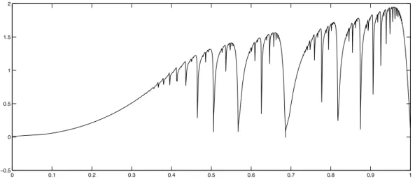
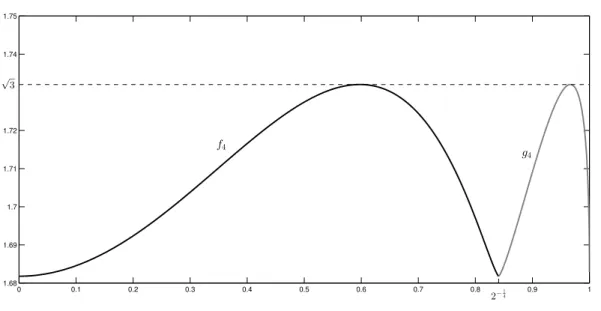
22 Chapter 1. The m-linear Bohnenblust–Hille and Hardy–Littlewood inequalities

i.e.,

Bmult

K,m,(λ0,s,...,s) (σK)

2m(m−1)

p 8Bmult R,m

9p−2m

p _{. (1.10)}

More precisely, (1.9) is valid with B_Kmult_{,m,(λ0,s,...,s)} as above.

Let λj = λ0p/(p−λ0j) for all j = 1, ...., m. Note that λm = s and that (p/λj)⇤ =

λj+1/λj for all j = 0, ..., m−1. Let us suppose that 1  k  m and that

0 @Pn

ji=1

n

P

b

ji=1

|T(ej1, ..., ejm)|

s

!1

sλk−11

A

1 λk−1

 Bmult

K,m,(λ0,s,...,s)kTk

is true for all continuous m-linear forms T : `n p ⇥

k−1 times · · · ⇥`n

p ⇥`n1 ⇥ · · · ⇥`n1 ! K and

for all i = 1, ..., m. Let us prove that

0 @Pn

ji=1

n

P

b

ji=1

|T(ej1, ..., ejm)|

s

!1 sλk1

A

1 λk

 B_Kmult_{,m,(λ0,s,...,s)k}T_k,

for all continuous m-linear forms T : `n<sub>p ⇥</sub> k<sub>· · · ⇥</sub>times `n_{p ⇥} `n<sub>1 ⇥ · · · ⇥</sub> `n_{1 !} K and for all

i= 1, ..., m.

The initial case (the case k = 0) is precisely (1.9) with Bmult

K,m,(λ0,s,...,s) as in (1.10).

Consider

T _{2 L}(`n<sub>p</sub>,k<sub>. . . , `</sub>times n

p, `n1, . . . , `n1;K)

and for each x ₂ B_`n

p define

T(x) _{: `}n p ⇥

k−1 times · · · ⇥`n

p ⇥`n1 ⇥ · · · ⇥`n1 ! K

(z(1), ..., z(m)) _7! T(z(1), ..., z(k−1), xz(k), z(k+1), ..., z(m)),

with xz(k) _{= (x}

jzj(k))nj=1. Observe that kTk ≥ sup{kT(x)k : x 2 B`n

p}. By applying the

induction hypothesis to T(x)_{, we obtain}

0 @Pn

ji=1

n

P

b

ji=1

|T (e_j1, ..., e_jm)_|s_|x_jk|s !1

sλk−11

A

1 λk−1

=

0 @Pn

ji=1

n

P

b

ji=1

&

&T 8e_j1, ..., e_jk−1, xe_jk, e_jk+1, ..., e_jm9&&s !1

sλk−11

A

1 λk−1

=

0 @Pn

ji=1

n

P

b

ji=1

&

&T(x)_(e

j1, ..., ejm)

& &s

!1

sλk−11

A

1 λk−1

 BKmult,m,(λ0,s,...,s)kT

(x)

k

 BKmult,m,(λ0,s,...,s)kTk, (1.11)

Chapter 1. Lower and upper bounds for the constants of the classical Hardy–Littlewood

inequality 23

We shall analyze two cases, namely, i= k and i ₆=k.

• i =k.

Since (p/λj−1)⇤ =λj/λj−1 for all j = 1, ..., m, we conclude that

0 @Pn

jk=1

n

P

b

jk=1

|T (ej1, ..., ejm)|

s

!1 sλk1

A 1 λk = 0 B @ n P

jk=1

n

P

b

jk=1

|T (e_j1, ..., e_jm)_|s

!1 sλk−1

✓

p λk−1

◆⇤1

C A

1 λk−1

1

✓

p λk−1

◆⇤ = -0 @ Pn

b

jk=1

|T(ej1, ..., ejm)|

s

!1

sλk−11

A

n

jk=1

-1 λk−1

✓

p λk−1

◆⇤

=

0 B @ sup

y2B_{`n p}

λk−1

n

P

jk=1 |yjk|

n

P

b

jk=1

|T (ej1, ..., ejm)|

s

!1 sλk−1

1 C A

1 λk−1

=

0 @ sup

x2B`n_p

n

P

jk=1

|x_jk|λk−1

n

P

b

jk=1

|T (e_j1, ..., e_jm)_|s

!1

sλk−11

A

1 λk−1

= sup

x2B`n_p

0 @Pn

jk=1

n

P

b

jk=1

|T (ej1, ..., ejm)|

s

|xjk|

s

!1

sλk−11

A

1 λk−1

 BKmult,m,(λ0,s,...,s)kTk

where the last inequality holds by (1.11).

• i ₆=k.

Let us first suppose that k _{2 {}1, ..., m₋1_}. It is important to note that in this case

λk−1 < λk < s for all k 2 {1, ..., m−1}. Denoting, for i = 1, ...., m,

Si = n

P

b

ji=1

|T(ej1, ..., ejm)|

s !1 s we get n P

ji=1

n

P

b

ji=1

|T(ej1, ..., ejm)|

s

!1 sλk

=

n

P

ji=1

Sλk

i = n

P

ji=1

Sλk−s

i Sis

= Pn

ji=1

n

P

b

ji=1

|T(ej₁,...,ejm)|s

S_is−λk = n

P

jk=1

n

P

b

jk=1

|T(ej₁,...,ejm)|s

24 Chapter 1. The m-linear Bohnenblust–Hille and Hardy–Littlewood inequalities

= Pn

jk=1

n

P

b

jk=1

|T(ej₁,...,ejm)| s(s−_λk) s−_λk−1

S_is−λk |T(ej1, ..., ejm)|

s(_λk−_λk−1)

s−_{λk−1 .}

Therefore, using H¨older’s inequality twice (first with the exponents (s ₋λk−1)/(s −λk)

and (s ₋ λk−1)/(λk −λk−1) and then next with λk(s −λk−1)/λk−1(s − λk) and λk(s −

λ_k−1)/s(λ_{k −}λ_k−1) we obtain

n

P

ji=1

n

P

b

ji=1

|T(e_j1, ..., e_jm)_|s

!1 sλk

 Pn

jk=1

2 6 4 n P b

jk=1

|T(ej₁,...,ejm)|s

S_is−λk−1

! s−_λk

s−_{λk−1 n}

P

b

jk=1

|T(e_j1, ..., e_jm)_|s

!λk−_λk−1

s−_λk−1

3 7 5



0 @Pn

jk=1

n

P

b

jk=1

|T(ej₁,...,ejm)|s

S_is−λk−1

! λk λk−1

1 A

λk−1 λk ·

s−_λk

s−_λk−1

⇥

0 @Pn

jk=1

n

P

b

jk=1

|T(e_j1, ..., e_jm)_|s

!1 sλk1

A

1 λk·

(_λk−_λk−1)s s−_λk−1

. (1.12)

We know from the case i= k that

0 @ Pn

jk=1

n

P

b

jk=1

|T(ej1, ..., ejm)|s

!1 sλk1

A

1 λk·

(_λk−_λk−1)s s−_λk−1

⇣Bmult

K,m,(λ0,s,...,s)kTk

⌘(_λk−_λk−1)s s−_λk−1

. (1.13)

Now we investigate the first factor of the right side in (1.12). From H¨older’s inequality (with the exponents s/(s₋λk−1) and s/λk−1) and (1.11) it follows that

0 @Pn

jk=1

n

P

b

jk=1

|T(ej₁,...,ejm)|s

S_is−λk−1

! λk λk−1

1 A

λk−1 λk = -P b jk

|T(ej₁,...,ejm)|s

S_is−λk−1

!n

jk=1

--✓ p λk−1

◆⇤

= sup

y2B_{`n p}

λk−1

n

P

jk=1

|y_jk| Pn

b

jk=1

|T(ej₁,...,ejm)|s

S_is−λk−1 = sup_x2B

`n_p

n

P

jk=1

n

P

b

jk=1

|T(ej₁,...,ejm)|s

S_is−λk−1 |xjk| λk−1

= sup

x2B`n_p

n

P

ji=1

n

P

b

ji=1

|T(ej₁,...,ejm)|s−λk−1

Ss_i−λk−1 |T(ej1, ..., ejm)| λk−1|x

jk|λk−1

 sup

x2B`n_p

n

P

ji=1

n

P

b

ji=1

|T(ej₁,...,ejm)|s

Ss i

!s−_λk−1

s _n

P

b

ji=1

|T(ej1, ..., ejm)|

s_|x jk|s

!1 sλk−1

= sup

x2B`np

n

P

ji=1

n

P

b

ji=1

|T(ej1, ..., ejm)|s|xjk|

s

!1 sλk−1

⇣Bmult

K,m,(λ0,s,...,s)kTk

⌘λk−1