MONO-TEMPORAL GIS UPDATE ASSISTANCE SYSTEM BASED ON UNSUPERVISED
COHERENCE ANALYSIS AND EVOLUTIONARY OPTIMISATION
Christian Becker, Joern Ostermann, Martin Pahl
Leibniz Universit¨at Hannover Institut f¨ur Informationsverarbeitung Appelstr. 9a, 30167 Hannover, Germany (becker, ostermann, pahl)@tnt.uni-hannover.de
http://www.tnt.uni-hannover.de
Commission IV/2
KEY WORDS:Land Cover, Updating, Change Detection, Semi-automation
ABSTRACT:
Data in Geo Information Systems (GIS) is used for map services and various applications. Thus, quality assessment on a regular basis is required to keep the data up-to-date. In this paper we focus on one key reasons for updates: incorrect object borders. State of the art systems semi-automatically analyse up-to-date satellite image data to narrow down areas that have to be considered forGIS updates. Often resources are limited and only data from one point in time is available that is compared to the data. Rule based systems are required to bridge the gap betweenGISspecifications and results from image analysis. We present a system that can find areas of change without any manual configuration. Our approach automatically learns about important aspects ofGISspecifications by analysing correctGISobjects. In potentially out-datedGISdata still a majority of objects is unchanged. Thus, we derive an model for normality (= correctness) by evaluating the coherence of relations betweenGISobjects and image analysis results. We synthesise changes atGIS object borders and analyse the impact on normality. In an evolutionary optimisation we determine areas of change that are rated with a significance value. We show that we can find 83% of all relevant update areas with a precision of 0.18, not considering the significance of changes. Including significance we can push the precision to 0.26 while still finding 77% of all relevant update areas.
1 INTRODUCTION
Up-to-date spatially referenced data is crucial for various appli-cations like urban planning, hazard management and agriculture (Lu et al., 2004). Such data usually is stored as data of a Geo Information System (GIS). Each data entry is stored as an geo referenced object, features of the entry are stored as attributes. A mandatory attribute is theGISfeatureto group object (eg. settle-ment or forest). Depending on the data, the shape may be spec-ified as lines, polygons or points. While gathering and updating spatial reference data can be a very complex task (eg. performing field surveys and in-depth studies), finding potentially out-dated areas can be simplified by evaluating land cover changes in re-mote sensing data like satellite images. Still, manual checks of satellite images is very time consuming. Hence, support through (semi-) automatic systems is requested. Approaches that use var-ious sensors and/or data for several have been developed (Lu et al., 2004). In many application only satellite images for a current point in time is available, though. In this mono-temporal setting images are analysed and results are compared to theGISdata to highlight potentially out-dated areas.
Existing systems can be divided into two groups: First, there are approaches that focus on image analysis methods for each con-sideredGISfeature. Afterwards the comparison with theGISdata is considered a trivial step (Lacroix et al., 2006),(Leignel et al., 2010). However, currently only for specialGISfeatures a reliable image analysis algorithm exists. Therefore, the correctness is of-ten considered a problem in a multi-feature environment. The lack of correctness inevitably leads to irrelevant areas for update. Hence, a second group of systems introduce an evaluation step to perform the comparison. Existing systems (Busch et al., 2004), (Buck et al., 2011) introduce for eachGISfeature manually con-figured rules in order to control the comparison. These systems can flexibly handle image analysis results, allowing to limit the
impact of only partial reliable results and to considerGISfeature specifications for determining update areas. On the other hand, rule sets can get too complex and unmanageable easily. More-over, to be able to compensate for complex image analysis results a rule designer needs to have knowledge of the characteristics of the result as well as ofGISspecifications (see Figure 1 for exam-ples ofGIS, image data and analysis results).
We show that important aspects ofGISspecifications can be au-tomatically and implicitly learnt from correctGISobjects. Since even it out-datedGISdata the vast majority of objects are still cor-rect, learning from correct objects is the same as learning from normal objects. A normality measure ofGIS objects is deter-mined by evaluating the coherence of relations between poten-tially out-datedGISdata and image analysis results. We already presented aGISobject based system in (Becker et al., 2012) . In this paper we concentrate on one of the main aspects of this scenario: incorrect object borders of existingGISobjects. This additional constraint allows us to enhance spatial resolutions of update areas to sub-object level. Using image analysis results we are able to sub-divideGISobjects into segments. By reassign-ing (or as we name it: switching) segments from oneGIS ob-ject to one of its neighbours we are able to synthesise expanded and shrunkenGISobjects. Evaluating the changes in normality caused by switches we are able to find update areas. In this pa-per we show that it is possible to use the squared Mahalanobis distance to implicitly express to what extent anGISobject com-plies toGISspecifications, using only the coherence of relations betweenGISobjects and image analysis results. We show that this can be used to replace rule based systems. Finally we show that using segments we are able to give update hints at sub-object level.
nor-Figure 1: Satellite image and image analysis result. Each colour represents a different kind of texture.GISobject borders describe theGISfeatures.
mality. This is required for Section 4 where we present how we model normality for the application to find incorrect object bor-ders. In Section 5 we describe the evolutionary algorithm that is used to find segments that describe areas of change. Results are presented and discussed in Section 6. Finally we summarise our contributions in Section 7.
2 TERMINOLOGY
By analysing georeferenced image data with existing computer vision algorithms, we obtain a pixel-wise classification. Each pixel is classified into one of several specificclasses. Intercon-nected pixels of the same class form georeferenced and classified
segments. They cover the same area in the scene as theGIS
ob-jects. Therefore, we say that everyGISobject iscomposed of (classified) segments and a segment isconnectedto aGISobject. To ensure that every segment is only connected to one specific GISobject, segments are split atGISobject borders. In our scene representation the location and extent of a (GIS) objectis only defined by the segments connected to the object. Since we are going to change the composition ofGISobjects we will name the state of compositions of all objects aconfigurationof the scene. When there is more than one scene, each scene is calledscene
version.
GISobject are composed of segments that are still represented as connections of pixels. While this representation is useful for vi-sualisation, an automatic system needs information to be present as numericalattributes. To describe the composition of aGIS ob-ject we developed suitable obob-ject attributes. To compare several objects they have to provide the same attributes. Segments don’t require any attributes (they still are classified, though).
3 MEASURING NORMALITY
In our system relations between aGISobject and image analysis results are described by a continuous multi-dimensional attribute vector, thus all objects form a continuous attribute space.
Segments for Update Relation Monitoring
Coherence Evaluation
Object Rating Up-To-Date Image Analysis Segments Out-Dated
GIS Objects
Recombination Selection
End of Iteration? Model
Scene Versions Scene
Evolutionary Optimisation
Coherence Analysis
Manual Postprocessing
Figure 2: Object Coherence Analysis and Update Detection by Evolutionary Optimisation.
The topic normality and abnormality in attribute space is known in the field ofdata mining(Tan et al., 2005). To estimate a nor-mality model, a large data set is required. We want to restrict the data basis for forming a statistical model of normality toGIS objects of the potentially out-dated input data set. Since the data may be partly incorrect the estimation of the model (some proba-bility distribution) needs to be robust.
Robustness can be enhanced by considering a priori knowledge. Since we don’t want to use configurations or rule sets, a-priority knowledge is rare, though. The only knowledge we assume is that GISobjects that belong to the sameGISfeature also look similar. Depending on theGISspecifications this might require consider-ing additionalGISattributes for sub-classification ofGISfeatures. Choosing an appropriate probabilistic distribution is also funda-mental to ensure robustness. We decided to use a multivariate Gaussian (normal) distribution to model the coherence of object attributes (= relations). The distribution’s parametersmeanand covariance matrix can be robustly estimated from large data sets. From our knowledge that aGISobject belongs to one of several GISfeatures, Gaussian distributions are estimated for each GIS feature independently. To determine distances in space with mul-tivariate Gaussian distributions we use the squared Mahalanobis distance:
d2mah(x, y) := (x−y)S
−1(x−y)T
(1)
whereSis the covariance matrix of the data. The Mahalanobis distance is a standard method for this application (Tan et al., 2005). The covariance matrixS in the formula is used to com-pensate pair-wise correlations between attributes. To interpret the squared Mahalanobis distance as normality measure, the distance of an object towards the Gaussian’s meanµmust be determined. Objects near the centre are more normal than more distant ob-jects. Thus, theabnormality valueof anGISobjectois calculated by
abnormality(o) :=d2mah(o, µ) (2)
0 ≤ abnormality <∞, using the mean and covariance matrix determined foro’sGISfeature. When we use in this paper the term highnormalitythis corresponds to a low abnormality value and vice versa. The absolute values of abnormality have no spe-cial meaning.
4 COHERENCE ANALYSIS
4.1 Relation Monitoring
To monitor relations between image segments andGISobjects we develop attributes. Since we want to determine normality ofGISobjects by using the squared Mahalanobis distance (see Section 3), we want the number of attributes to be small. A large number of attributes would require a very large number of samples to robustly approximate mean and covariances. The at-tributes should also be quite general so that all objects can be sensibly described by them. Finally, they should only reflect rel-evant information.
For our application we definedSegment Histogram Attributes. We will use the notation for sets as segments are connected pix-els. Operation|s|measures the size of a segmentsin pixels, the size of the an object is the sum of sizes of the segments connected to the object.
For eachGISobjectoand all segment classesi = 1,2, . . . , n attributesa1, a2, . . . , anare calculated so that
ai(o) := P
s∈Segmentsδi(s)|g∩s|
|o| (3)
with
δi(s) := (
1 ifshas segment classi
0 else (4)
Segment Histogram Attributesare invariant towards size so that
aGISobject will not be unusual due to its size only. If the size were a major factor, it could be checked in a pre-processing step easily, usingGISdata only.
4.2 Coherence Evaluation
The stepCoherence Analysisevaluates the attribute space spaned by theSegment Histogram Attributesof all objects. Therefore, for eachGISfeature the mean and covariance matrix are estimated. This allows determining the squared Mahalanobis distance (sec-tion 3) for eachGISobject with respect to its ownGISfeature. Means and covariance matrices are thenormality modelfor the algorithm. It will remain fixed for the rest of the algorithm.
5 EVOLUTIONARY OPTIMISATION
Now that we have gained an understanding of howGISobjects are supposed to be composed of segment classes it is possible to rate an object’s normality by calculating its squared Mahalanobis distance. However, an object rating neither provides update areas at sub-object level, nor does it specifically detect errors caused by incorrect object borders. Both can be achieved in our system by evaluating the effects when a segment is switched from oneGIS object to a neighbouring object. If the abnormality decreases, the switched segment is considered an update area. The difference of normality before and after the switch is called thesignificanceof the switch.
How many configurations have to be tested to check for all pos-sibilities so that all objects may have best normality? Given the application there is no reason to limit switches to just segments that initially touch a border of aGISobject. If major changes took place, an area described by a group of connected segments could have changed.
We formulate the following conditions that a segment must com-ply to in order to be considered as a candidate for a switch:
• Only segments that touch the border of aGISobject are able to switchGISobjects. OtherwiseGISobjects would not be growing from their borders.
• Every segment may only switch once in the whole optimisa-tion. This is done to ensure that aGISobject cannot “move” in the scene. Furthermore within several iteration steps aGIS object might interchange segments withGISobjects that are not immediate neighbours.
Every segment switch results in changes in object borders so that every switch the segments that fulfil the restrictions above change. This makes it very difficult to determine an order of op-timisation. Therefore we decided to implement an evolutionary algorithm.
Evolutionary algorithms (De Jong, 2002) are global optimisation algorithms. A evolutionary algorithm starts with an initial (not optimal) solution that is used to generate an initial set of possible solutions (called ageneration) by simple duplication. Each solu-tion in a generasolu-tion is then modified independently. The modifi-cations are evaluated to be able to select candidates that are going to be duplicated to form the next generation. Advantages are easy implementation and formulation of optimisation tasks especially for large data sets where brute force algorithms are too complex (like in our case). The downside of a evolutionary algorithms is that the quality of the result cannot be guaranteed. Depending on the application the selection process can be designed to limit this vulnerability to get stuck in an local optimum. Finally, like in all iterative algorithms some ending condition is required.
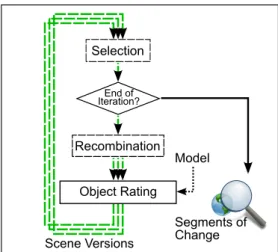
In the systems flow chart in Figure 2 our evolutionary algorithm is highlighted by a red border. An excerpt of the flow chart showing the evolutionary circle only is shown in Figure 3.
In our system a generation consists ofscene versions. We are working with a flexible generation size. While at the start of every iteration the number of scene versions is reduced to just a single scene version, within an iteration the number of scene version is increased dynamically.
5.1 Initialisation
The iterating process starts with an evaluation of the current state of the initial scene’s configuration. For each object theSegment
Histogram Attributes (Equation 3) are determined and its
nor-mality is evaluated by determining the abnornor-mality value (Equa-tion 2) using the appropriate model (sec(Equa-tion 4). In the first itera-tion theEnd of Iterationstep is skipped. Finally, the evolutionary circle is ready to start.
5.2 Selection
In this step it is decided which of the available scene versions will be used for further changes. The evaluation of a scene ver-sion’s configuration is done by summing up the abnormality value (Equation 2) of all of its objects. The scene version with the smallest sum of abnormalities is selected. The scene versions with a higher sum are discarded.
5.3 End of Iteration Check
Segments of Change Scene Versions
Object Rating Recombination
Selection
End of Iteration?
Model
Figure 3: Flow chart showing the system’s evolutionary part after initialisation.
5.4 Recombination
In the recombination step a segment is randomly chosen from the incoming scene version. First, the segment is checked against the conditions of candidates for a change (see Section 5). If the segment fails the check, another segment is chosen randomly.
To find the options for a change, all neighbouring segments are taken into account. Only neighbours with anotherGISfeature than the chosen segment are considered, though. (We want to de-tect changes in land usage, so there is no point in switching seg-ments between objects of the same features). This also includes segments connected to the sameGISobject. Now for each neigh-bouring segment left, the original scene is duplicated and a switch is performed: First, theGISobject connected to the neighbouring segment is determined. Afterwards the segment’s connection to its currentGISobject is removed, then a connection to the neigh-bour segment’s object is created.
The original scene version and all new versions are the new gen-eration of scene versions.
5.5 Object Rating
For each scene version, the changed object’sSegment Histogram
Attributes(equation 3) are updated and its normality is
evalu-ated (see Section 5.1). Additionally, for each switched segment, changes in normality are stored since we use it to rank the signif-icance of the switch.
5.6 System Output
The output of the systems are segments that have changed when compared to the initial scene version.
6 RESULTS AND DISCUSSION
In this section we present experimental results for our system. The test area is located in central Germany. IKONOSimagery with 1 m resolution on four channels (red,green,blueandnear
infrared) is available for image analysis to determine segments.
The image analysis is not part of this contribution. To highlight the performance of our new approach, we only use basic image analysis results calculated by aSupport Vector Machine(SVM), (Vapnik, 2000) withRBFkernel. Features aremean,covariance
andHaralick features(Haralick et al., 1973) in a25×25pixel
region. For performance reasons, every eighth pixel is classified,
only. Original resolution is gained though nearest neighbouring up scaling. We have trained theSVMwith samples industry halls, forest, small houses and grass/cropland. The test area is located in central Germany.GISdata is taken from the GermanGISdata set ATKIS(ATKIS, 2011). We selected the most prominentGIS fea-tures 2111 (settlement), 2112 (industry), 4101 (cropland), 4102 (grassland), 4107 (forest).
Reference Results Unfortunately, there are no benchmark sys-tems available for generalGISquality assessment systems. Thus we had to created a new reference data set to evaluate our system. We decided to label input segments as correct and incorrect by an independent person. Since the whole scene consists of roughly 25000 segments, 100GISobjects with 1008 segments have been randomly selected for a check. The reference found 42 relevant updates.
To evaluate the performance several error measures are deter-mined. First, we define following terms:
Update Segment Segment that is regarded as area where this GISobject needs to be updated.
True Update Segment Update segment according to the refer-ence.
Potential Update Segment Update segment that has been deter-mined as update segment by the system. In this section sev-eral aspects of the system are evaluated. It depends on the evaluation if an segment is regarded an update segment.
Basic measures show to which amount system and the indepen-dent reference agree:
True Positives (tp) Number of potential update segments that are true update segments.
False Positives (fp) Number of potential update segments that are not true update segments.
True Negatives (tn) Number of segments that are no potential update segment and to true update segment.
False Negatives (fn) Number of true update segments that are no potential update segments.
6.1 Evaluation ignoring Significance of Switches
Only considering switched segments as potential update segments we get following results:
❵ ❵
❵ ❵
❵ ❵
❵ ❵
❵ ❵❵
System
Reference Update Segments
No Update Segments
Update Segments tp: 35 fp: 162
No Update Segments fn: 7 tn: 804
The basic measures can be used to calculate measures that ex-press the trade off between tp, fp, tn, fn:
Precision= tp
tp+fp, 0≤Precision≤1 (5)
Recall= tp
On the one hand, high precision means that only relevant infor-mation has to be checked, in our case that many potential update segments are true update segments. It does not tell how many true update segments are not potential update segments. On the other hand, high recall indicates that nearly all true update segments are potential update segments. However, there is no indication about the number of potential update segments without being an true update segment.
Results are: Precision =0.18, Recall =0.83.
6.2 Evaluation of Significance of Switches
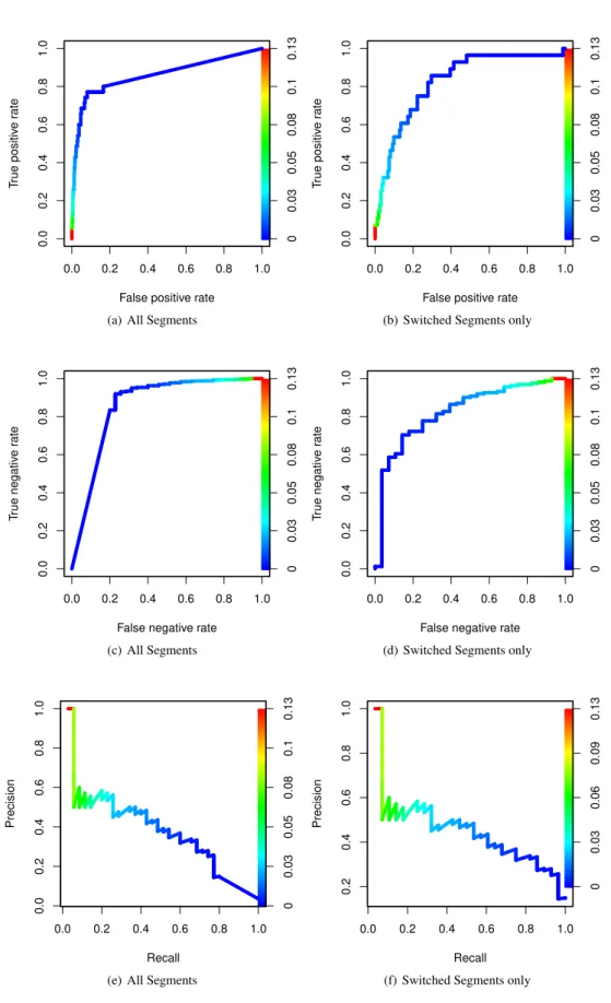
Switched segments are rated by their significance value (Sec-tion 5.5) that can be used to improve precision or recall. Measures of last section can still be determined but they depend on specific significance values so they are expressed as graphs. True/false positives are displayed in Figures 4 (a), (c) and (e). Since true and false positives/negatives are strongly connected, each pair is expressed in a common graph. Each point on the curve results from determining true and false positives/negatives for a specific significance threshold. The value of the threshold is colour coded, the legend can be seen as colour bar at the right axis. To include also segments that have been missed by the system, we assigned them a significance of−0.0001so they are all equal and lower in significance then any switched segment. For better visualisa-tion, we provide graphs only for switched segments in Figures 4 (b), (d) and (f). It can be easily seen that switched segments with the lowest significance are mostly non-true update segments. In other words: when ignoring segments with a slightly positive sig-nificance as potential updates, the number of false positives drops by roughly from 162 to 51 while only three additional true pos-itive objects haven been missed. This effect can also be seen in Figures 4 (e) and (f). Precession can be strongly increased with-out much loss in recall. A similar effect can be seen considering the true and false negative figures which is remarkable consider-ing that only 42 of 1008 segments are true update segments.
In a real application, of course, no graph is available to select an optimal significance value. In this case we propose to check potential update segments starting with the highest significance. As can be seen the frequency of finding true update segments is very high compared to the frequency with low significance.
7 CONCLUSIONS
UpdatingGISdata is of major interest for many applications, but is a very complex and time consuming task. This paper deals with one major source of changes: incorrectGISobject borders. Existing quality assessment systems follow rather uniform ap-proaches that introduce complex rule sets. We propose to change the procedure from rule based into an automatic evaluation. We demonstrate how a normality model for relations between image analysis results andGISobjects, based on squared Mahalanobis distances, is used to replace knowledge that in existing systems is introduced by rules.GISobjects are sub-divided into segments of specific image analysis classes. Relations betweenGISdata and segments are described by object wise determining distribu-tions of analysis classes. Finally, evolving the scene by switching segments betweenGISobjects and monitoring the changes in dis-tributions and normality we identify segments that are probable changes at sub-object level. In addition, proposed updated seg-ments are rated with a significance value.
This paper shows that rule based systems can be replaced by an automatically evaluation. Lowering requirements for human op-erators and providing areas for proposed updates at sub-object
level the scope of application exceeds the scope of existing sys-tems. We show that using only basic image analysis, 83 % of all update areas could be found with more than every sixth pro-posed update is a relevant update. Considering the significance value, only checking less than every fourth proposed segment still around 77 % of relevant segments could be found. Our system is not meant to be an alternative to cutting-edge image analysis, though. Without any question, results would further benefit from using more elaborate image analysis methods. However, this also applies in the opposite direction: using our system, image sis methods can be developed that focus on general image analy-sis tasks instead of dealing with specificGISfeature definitions.
REFERENCES
ATKIS, 2011. Amtliches Topographisch-Kartographisches Infor-mationssystem.
Becker, C., Pahl, M. and Ostermann, J., 2012. Automatic quality assessment of gis data based on object coherence. GEOBIA 2012.
Buck, O., Peter, B. and B¨uker, C., 2011. Zwei-skaliger ansatz zur aktualisierung landwirtschaftlicher referenzkulissen (lpis). Photogrammetrie - Fernerkundung - Geoinformation PFG, E. Schweizerbart’sche Verlagsbuchhandlung 5(5), pp. 339–348.
Busch, A., Gerke, M., Gr¨unreich, D., Heipke, C., Liedtke, C.-E. and M¨uller, S., 2004. Automated verification of a topographic reference dataset: System design and practical results. Interna-tional Archives of Photogrammetry and Remote Sensing XXXV, Part B2, pp. 735–740.
De Jong, K. A., 2002. Evolutionary Computation: A Unified Approach. 1st edn, The MIT Press.
Haralick, R. M., Shanmugam, K. and Dinstein, I., 1973. Textural features for image classification. Systems, Man and Cybernetics, IEEE Transactions on 3(6), pp. 610 –621.
Lacroix, V., Idrissa, M., Hincq, A., Bruynseels, H. and Swarten-broekx, O., 2006. Detecting urbanization changes using spot5. Pattern Recognition Letters 27(4), pp. 226 – 233. Pattern Recog-nition in Remote Sensing (PRRS 2004).
Leignel, C., Caelen, O., Deibeir, O., Hanson, E., Leloup, T., Sim-ler, C., Beumier, C., Bontempi, G., Warz´ee, N. and Wolff, E., 2010. Detecting man-made structure changes to assist geographic data producers in planning their update strategy. ISPRS Archive Vol. XXXVIII, Part 4-8-2-W9.
Lu, D., Mausel, P., Brond´ızio, E. and Moran, E., 2004. Change detection techniques. International Journal of Remote Sensing 25(12), pp. 2365–2401.
Tan, P.-N., Steinbach, M. and Kumar, V., 2005. Introduction to Data Mining, (First Edition). Addison-Wesley Longman Publish-ing Co., Inc., Boston, MA, USA.
False positive rate
T
rue positiv
e r
ate
0.0 0.2 0.4 0.6 0.8 1.0
0.0
0.2
0.4
0.6
0.8
1.0
0
0.03
0.05
0.08
0.1
0.13
(a) All Segments
False positive rate
T
rue positiv
e r
ate
0.0 0.2 0.4 0.6 0.8 1.0
0.0
0.2
0.4
0.6
0.8
1.0
0
0.03
0.05
0.08
0.1
0.13
(b) Switched Segments only
False negative rate
T
rue negativ
e r
ate
0.0 0.2 0.4 0.6 0.8 1.0
0.0
0.2
0.4
0.6
0.8
1.0
0
0.03
0.05
0.08
0.1
0.13
(c) All Segments
False negative rate
T
rue negativ
e r
ate
0.0 0.2 0.4 0.6 0.8 1.0
0.0
0.2
0.4
0.6
0.8
1.0
0
0.03
0.05
0.08
0.1
0.13
(d) Switched Segments only
Recall
Precision
0.0 0.2 0.4 0.6 0.8 1.0
0.0
0.2
0.4
0.6
0.8
1.0
0
0.03
0.05
0.08
0.1
0.13
(e) All Segments
Recall
Precision
0.0 0.2 0.4 0.6 0.8 1.0
0.2
0.4
0.6
0.8
1.0
0
0.03
0.06
0.09
0.13
(f) Switched Segments only