Research and Politics April-June 2016: 1 –13 © The Author(s) 2016 DOI: 10.1177/2053168016643345 rap.sagepub.com
Creative Commons CC-BY: This article is distributed under the terms of the Creative Commons Attribution 3.0 License (http://www.creativecommons.org/licenses/by/3.0/) which permits any use, reproduction and distribution of
the work without further permission provided the original work is attributed as specified on the SAGE and Open Access pages (https://us.sagepub.com/en-us/nam/open-access-at-sage).
In a recent issue of Political Analysis, Taylor Grant and Matthew Lebo author the lead and concluding articles of a symposium on time series analysis. These two articles argue forcefully against the use of the general error correc-tion model (GECM). In their lead article, Grant and Lebo declare: “we recommend the GECM in only one rare situa-tion: when all of the variables are strictly unit-root series, Y
t is unbounded, Yt and Xt are cointegrated, and the MacKinnon critical values are used… A careful look at the applied literature in political science will not find any examples that meet all those criteria” (p.27). They reiterate this point in their concluding article, stating: “we remain skeptical that the GECM is a reliable model except in the very rare case where one has unbounded unit-root variables that are cointegrated with each other” (p.80). Given the popularity of the GECM for time series analysis (e.g. Beck and Katz, 2011; Blaydes and Kayser, 2011; Jennings, 2013; Layman et al., 2010; Soroka et al., 2015), Grant and Lebo’s insistence that the GECM is inappropriate for political sci-ence applications would seem to hold major implications for time series practitioners.1
Grant and Lebo identify two primary concerns with the GECM. First, when time series are stationary, the GECM cannot be used as a test of cointegration. This is a useful and often under-appreciated point.2 However, if this were Grant and Lebo’s only concern, their analysis would not fundamentally alter the conclusions of past research and could be easily dealt with in future studies by not using the GECM to test for cointegration with stationary time series. Grant and Lebo’s second concern is much more troubling. They argue that across most (and perhaps all) political sci-ence time series, the GECM will produce “an alarming rate of Type I errors” (p.4). This threat of spurious findings is
Don’t jettison the general error correction
model just yet: A practical guide to
avoiding spurious regression with
the GECM
Peter K. Enns
1, Nathan J. Kelly
2, Takaaki Masaki
3and
Patrick C. Wohlfarth
4Abstract
In a recent issue of Political Analysis, Grant and Lebo authored two articles that forcefully argue against the use of the
general error correction model (GECM) in nearly all time series applications of political data. We reconsider Grant and Lebo’s simulation results based on five common time series data scenarios. We show that Grant and Lebo’s simulations (as well as our own additional simulations) suggest the GECM performs quite well across these five data scenarios common in political science. The evidence shows that the problems Grant and Lebo highlight are almost exclusively the result of either incorrect applications of the GECM or the incorrect interpretation of results. Based on the prevailing evidence, we contend the GECM will often be a suitable model choice if implemented properly, and we offer practical advice on its use in applied settings.
Keywords
time series, ecm, error correction model, spurious regression, methodology, Monte Carlo simulations
1Cornell University, USA 2University of Tennessee, USA 3College of William & Mary, USA 4University of Maryland, College Park, USA
Corresponding author:
Nathan J. Kelly, University of Tennessee, 1001 McClung Tower, Knoxville, TN 37996-0410, USA.
Email: [email protected]
the primary reason Grant and Lebo advocate abandoning the GECM.
If the GECM regularly produces spurious results, schol-ars would indeed be well-advised to abandon this approach. However, the problems Grant and Lebo highlight follow almost entirely from either incorrect applications of the GECM or incorrect interpretation of results. Indeed, a care-ful examination of Grant and Lebo’s results, as well as the other contributions to the Political Analysis symposium, shows the GECM performs quite well across a variety of common data scenarios in political science. In this article, we examine five of the scenarios that Grant and Lebo con-sider and we find that for four of the data scenarios, if applied correctly the GECM can be estimated without con-cern for spurious relationships. With the fifth data type (fractionally integrated series), the GECM sometimes offers a suitable approach.3 Our analysis pays particularly close attention to the cases of bounded unit roots and near-integrated time series. We devote extra attention to these types of time series because they are common in political science and because none of the other symposium articles reconsider Grant and Lebo’s claims about these types of data.4 We show that when applied correctly, there is no inherent problem when using the GECM with bounded unit roots or near-integrated data.
Although our conclusions differ greatly from Grant and Lebo’s recommendations, we do not expect our findings to be controversial. Most of our evidence comes directly from Grant and Lebo’s own simulations. We also support our claims with additional simulation results. Although our findings are straightforward, our conclusions about the GECM are important for multiple reasons. First, a correct understanding of the GECM holds implications for how we understand existing research. Grant and Lebo identified five prominent articles and in each case they critiqued the authors’ use of the GECM. Grant and Lebo also pointed out that none of the other symposium articles provide “a defense of any GECM results published by a political sci-entist” (p.70). Our findings show that Grant and Lebo were too quick to criticize these researchers’ use of the GECM. Indeed, we reconsider two of the articles that Grant and Lebo critiqued (Casillas et al., 2011; Kelly and Enns, 2010) and we demonstrate that a correct understanding of the GECM indicates that the methods and findings of these two articles are sound.
Understanding the GECM also holds implications for future research. For time series analysis, Grant and Lebo recommend fractional integration (FI) methods. Although FI methods are certainly an important statistical approach (e.g. Box-Steffensmeier et al., 1998; Box-Steffensmeier and Tomlinson, 2000; Clarke and Lebo, 2003), substantial disagreement exists regarding their utility for political sci-ence data (Box-Steffensmeier and Helgason, 2016).5 Given the debate about the utility of FI methods (especially with short time series), it is important for researchers to know
when the GECM avoids the errors that Grant and Lebo ascribe to it. Until alternate methods are shown to perform better, based on our findings we recommend that research-ers use the GECM for bounded unit roots (when statistical tests indicate the dependent variable contains a unit root and cointegration is present) and with near-integrated data (again, cointegration must be established when statistical tests suggest a unit root).6 We also remind readers that the GECM is appropriate with FI data in some contexts (Esarey, 2016; Helgason, 2016) and it is appropriate with stationary time series (although we point out that the mathematically equivalent autodistributed lag model (ADL) is less likely to produce errors of researcher interpretation with stationary data).
We conclude with a detailed summary of our recommen-dations for time series practitioners, highlighting where we agree with Grant and Lebo and where our recommenda-tions differ. The conclusion also discusses avenues for future research. These include studying the performance of the GECM with other types of time series. Wlezien (2000), for example, discusses “combined” time series (which con-tain both integrated and stationary processes) and he shows they can be modeled with a GECM. Future research also needs to continue to evaluate the performance of FI tech-niques. Of particular interest is resolving the debate between Lebo and Grant (2016) and Keele et al. (2016) regarding how long a time series must be to reliably esti-mate the FI parameter d and demonstrating whether Grant and Lebo’s proposed fractional error correction model (FECM) is able to identify true relationships in short time series.
Reconsidering five of Grant and Lebo’s
data scenarios
In this section, we revisit Grant and Lebo’s first five data scenarios. We find that across all five scenarios, the GECM typically avoids spurious relationships. We explain why our results differ from Grant and Lebo’s conclusions and highlight when we agree with their recommendations.
Case 1: The dependent variable contains a unit
root,
ɪ
(1)
Grant and Lebo begin with a very important, and often for-gotten, point. They show that if the dependent and inde-pendent variables contain a unit root, cointegration must be established prior to interpreting the results of a GECM (see also Enns et al., 2014).7 Grant and Lebo explain, “Without cointegration, however, the model is unbalanced and the practitioner should set aside the estimates and choose a different specification” (p.7).8 Grant and Lebo also correctly emphasize that when Yt contains a unit root and the GECM
values must be used (Ericsson and MacKinnon, 2002) to evaluate cointegration” (p.8). Specifically, the t -statistic associated with α1 (i.e. the error correction rate) in the GECM
∆Y Y ∆X X
t=α0+α1 t−1+β0 t+β1 t−1+εt, (1)
must be less than the corresponding critical value in Ericsson and MacKinnon (2002). Grant and Lebo’s Table 2 (second row) confirms that when an analyst uses the appro-priate critical values, this cointegration test performs well even when T = 60 and regardless of the number of predic-tors specified in the model. Since Grant and Lebo only find (incorrect) evidence of cointegration about 5 per cent of the time, if researchers follow Grant and Lebo’s recommenda-tion to set aside estimates when there is no evidence of cointegration, incorrect evidence of a long-run relationship (i.e. β1 in Equation (1)) could never exceed 5 per cent with integrated data (because 95% of potential analyses have been set aside).
At first glance, the bottom row of Grant and Lebo’s Table 2 might appear to contradict this statement, because these results show that Grant and Lebo incorrectly rejected the null hypothesis that β1= 0 after testing for cointegra-tion between 14 and 47 per cent of the time. However, these results are based on cointegration tests with incorrect criti-cal values.9 Thus, the bottom row of Grant and Lebo’s Table 2 should be read as evidence of the importance of using the correct MacKinnon critical values when testing for cointegration, not evidence of spurious relationships with the GECM. Their Table 2 also shows that although α1 provides accurate tests of cointegration (when researchers use the correct critical values), α1 (which typically ranges between 0 and −1.0) is biased downward (i.e. more nega-tive). Typically, this bias will not pose a problem for researchers. First, the bias does not affect the estimates of
β0 or β1 (because these estimated short- and long-run
effects do not depend on α1). Second, the magnitude of the bias is small.10 Third, the bias influences the estimate of the total effect of Xt on Yt (i.e. the long-run multiplier (LRM)) in a conservative direction. The conservative bias emerges because a smaller (more negative) α
1 will decrease the estimated LRM (because the LRM equals β
α 1
1
), leading
researchers to conclude a smaller total effect of Xt on Yt.
Because α1 indicates how quickly the total effect of Xt on Yt occurs through future time periods, researchers must also be aware that if α1 is biased downward, the true rate of error correction likely takes longer than α1 implies. When discussing the LRM or the rate of error correction, research-ers must acknowledge how the bias in α1 that Grant and Lebo identified could affect their estimates. However, as long as researchers acknowledge this bias in α1, we agree with Grant and Lebo that the GECM can be used with inte-grated data that are cointeinte-grated.
Case 2: The dependent variable is a bounded
unit root
Grant and Lebo’s second case considers bounded unit roots, which are time series that “can exhibit the perfect-memory of integrated data” but are bound between an upper and lower limit (p.10). Grant and Lebo cite the public’s policy mood as an example (Stimson, 1991). They find that policy mood contains a unit root, but because it is based on survey per-centages, it is clearly bound between 0 and 100. According to Grant and Lebo, bounded unit roots should not be ana-lyzed with a GECM. They write, “Even if we find series that are strictly unit-roots and we use MacKinnon CVs, mistakes are still rampant if our dependent variable is one of the vast majority of political times series that is bounded” (p.12).
A reconsideration of Grant and Lebo’s simulations dem-onstrates, however, that the GECM performs no worse with bounded unit roots than it does with the integrated time series discussed in Case 1 (where Grant and Lebo recommend the use of the GECM). First, consider Grant and Lebo’s finding that, “Boundedness does not seem to affect the estimation of β1 or β0” (pp.11–12). This is an important result because these parameters correspond with the long-run and immedi-ate relationships between Xt and Yt, which are typically
what researchers are most interested in testing. Grant and Lebo’s concern is that the GECM yields incorrect inferences about cointegration with bounded unit roots. Consistent with this claim, their Table 3 shows that the GECM incorrectly shows evidence of cointegration between unrelated series more than 5 per cent of the time. However, the inflated rate of Type I errors associated with the cointegration test results because of an incorrect application of the GECM.11
To understand why the results in Grant and Lebo’s Table 3 are problematic, recall that Grant and Lebo’s key point about bounded unit roots is that despite containing a unit root, bounded unit roots behave differently than pure I(1)
series. Specifically, “as the series nears its upper and lower thresholds it tends towards mean reversion” (Grant and Lebo, Supplementary Materials, p.13). This mean reversion at set bounds can produce a constant mean with a constant variance, which means the series would behave as if station-ary. If the series behaves as if it is stationary, even if the data generating process (DGP) contains a unit root, these sample properties must inform the statistical analysis. As Grant and Lebo write, “Analysts should deal with the properties of the data sample they have and not make arguments about asymp-totics” (p.72).12 Thus, even if we know the DGP to contain a unit root, if the bounded nature of the data produces a series that mimics a stationary time series, we must take this into account.
rather simple modeling strategy for bounded unit roots. When a bounded unit root behaves as if it is stationary, the GECM should not be used to test for cointegration. When a bounded unit root behaves as if it contains a unit root, the GECM should be appropriate. To test whether this strategy avoids Type I errors, we replicate Grant and Lebo’s bounded unit root simulations, adding a test for the time series prop-erties of Yt. Specifically, we use Grant and Lebo’s simulation
code to generate dependent series to be bounded unit roots. These series depend on three parameters: the range of the bounds, which is set to 1–100 and 49–71, the variance of the disturbance term, which is set to 1, 2, or 3, and the series length, where T equals 60, 100, or 150.13 Following Grant and Lebo, the predictors are integrated time series I(1).
After generating these series, we use an augmented Dickey Fuller (ADF) test to evaluate whether we reject the null hypothesis of a unit root in the dependent series. At first, our use of an ADF test may seem surprising. It is well known that ADF tests are underpowered against the alter-native hypothesis of stationarity (Blough, 1992; Cochrane, 1992). Thus, the ADF may incorrectly conclude that a series that behaves as if stationary follows a unit root pro-cess in the observed data. However, this means we are bias-ing our simulations against support for the GECM since we are more likely to incorrectly conclude the series contains a unit root and thus inappropriately utilize the GECM as a test of cointegration (thereby inflating the rate of Type I errors with those cointegration tests). If the ADF rejects the null of a unit root, we do not use the GECM to test for coin-tegration. Even though the true DGP in our simulations is a bounded unit root, if the series behave as if stationary (because the bounds and mean reversion generate a series with a constant variance and mean), the GECM should not be used to test for cointegration. Not only would the cointe-gration test be wrong if the dependent series behaves as if stationary, but we have no reason to expect a cointegrating relationship between an integrated predictor and an out-come variable that appears stationary (Keele et al., 2016).
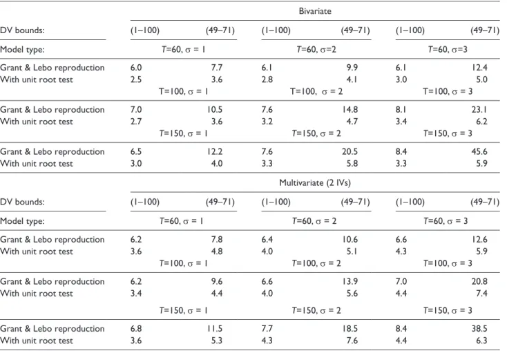
Table 1 reproduces Grant and Lebo’s original results (from their Table 3, p.11) and the results from our simula-tions. Recall that our simulations are identical to Grant and Lebo’s except we do not use the GECM to test for cointe-gration if an ADF test on Yt rejects the null of a unit root.
We add this step because a stationary time series cannot be cointegrated with an integrated time series (Keele et al., 2016), rendering it unnecessary to test for cointegration, and because tests for cointegration with a stationary time series will produce biased results (Grant and Lebo, 2016). First, note that Grant and Lebo’s results show that naively estimating a GECM will produce incorrect evidence of cointegration more than 5 per cent of the time, and these errors will increase as T increases, the variance increases, and with the more limited bounds of 49 to 71. These results are not surprising because as discussed above, each of these conditions (i.e. longer T, greater variance, and narrower bounds) would increase the mean reversion of the series.
Our primary interest is evaluating whether the GECM yields correct inferences if we first test the sample proper-ties of the bounded unit root. To test this expectation, the “With Unit Root Test” rows only use the GECM to test for cointegration if the ADF test does not reject the null hypoth-esis of a unit root in the dependent series. Across all param-eters, the Type I error rate is about 5 per cent. By first diagnosing the time series properties of the dependent series (which is standard practice in time series analysis), we avoid the Type I errors in the cointegration tests. These results show that there is no inherent problem with using the GECM with bounded unit roots.14 This is an important result. Grant and Lebo state, “Even if we find series that are strictly unit-roots and we use MacKinnon CVs, mistakes are still rampant if our dependent variable is one of the vast majority of political times series that is bounded” (p.12). Yet, the results in Table 1 show that if we follow these guidelines (i.e. find evidence of unit–roots and use MacKinnon critical values), the mistakes Grant and Lebo found essentially disappear.
In addition to offering guidance about the appropriate use of the GECM, these simulation results hold implications for Grant and Lebo’s analysis of Kelly and Enns (2010). Grant and Lebo use Kelly and Enns’ analysis of the relationship between income inequality and policy mood to illustrate the pitfalls of analyzing a bounded unit root with a GECM. Specifically, based on Kelly and Enns’ analysis, Grant and Lebo conclude that there is “No cointegration” and thus the “GECM model [is] inappropriate” (p.26). Yet, looking at Kelly and Enns’ most parsimonious analysis (Table 1, Column 2) we find clear evidence of cointegration.15 We select the most parsimonious specification because in Keele, Linn, and Webb’s first contribution to the symposium, they suggested that Kelly and Enns over-fit their model. By focusing on this parsimonious model (which Keele, Linn, and Webb did not consider) we mitigate concerns that the results are due to over-fitting the model. The evidence of cointegration in Kelly and Enns’ analysis combined with the simulation results above in Table 1 support the use of the GECM. Grant and Lebo also conclude that there is “No sup-port for short- or long-term effect of income inequality on public mood” (p.26). This conclusion is surprising because, as noted above, Grant and Lebo conclude that “Boundedness does not seem to affect estimation of β1 or β0” (pp.11–12) and β0 and β1 reflect Kelly and Enns’ estimates of the
short- and long-term relationships between income inequal-ity and public mood (see Grant and Lebo’s Equation (5)). Grant and Lebo’s conclusion that the estimates of β0 and β1 are not affected by boundedness further validates Kelly and Enns’ estimates of these parameters.
for variables that are surely unrelated to the public’s policy mood: beef consumption, coal emissions, tornado fatalities, and onion acreage (see Grant and Lebo’s Table E.13). Grant and Lebo write, “Based on our past replications and simula-tions we expect spurious regressions, and that is what we find” (Grant and Lebo, supplementary materials, p.43). This conclusion depends, however, on an incorrect applica-tion of the GECM. Across the eight nonsense regressions, none show evidence of cointegration.16 If Grant and Lebo followed their own advice to “set aside the estimates” with-out cointegration, they would never have reported these results from these nonsense regressions.17 The spurious results in their nonsense regressions result because they did not test for cointegration. We should also note that even if the GECM was implemented correctly, we do not recom-mend the use of atheoretical variables to demonstrate the possibility of spurious findings. Instead, we recommend the standard approach of simulating data and conducting Monte Carlo experiments.18
Grant and Lebo’s final critique of Kelly and Enns comes from their Tables E.16 and E.17, where they re–analyze Kelly and Enns’ data with a FECM and find no significant
relationships in the data. What Grant and Lebo fail to con-sider is the possibility that FECMs under-identify true rela-tionships in small samples. Since Grant and Lebo’s fractional differencing analyses failed to fully replicate four out of five influential articles, this is a critical consideration. In all of their simulations, Grant and Lebo never report how often fractional differencing methods identify true relationships. Helgason (2016) considered prediction error and found that the performance of the FECM depends heavily on whether short-term dynamics are present and the sample size, but he did not test how often FECMs correctly identify true rela-tionships. We also do not know how the FECM performs if applied to data that are not fractionally integrated. If the FECM is overly conservative, Grant and Lebo’s re-analysis and critiques of the other articles would also be highly prob-lematic. This is an important area for future research.
Case 3: The dependent variable and all
independent variables are stationary
As we noted earlier, Grant and Lebo make an important contribution by highlighting the fact that α1 in a GECM Table 1. The percentage of simulations that provide incorrect evidence of cointegration based on Grant and Lebo’s Table 3 and based on first testing for a unit root.
Bivariate
DV bounds: (1–100) (49–71) (1–100) (49–71) (1–100) (49–71)
Model type: T=60, σ = 1 T=60, σ=2 T=60, σ=3
Grant & Lebo reproduction 6.0 7.7 6.1 9.9 6.1 12.4
With unit root test 2.5 3.6 2.8 4.1 3.0 5.0
T=100, σ = 1 T=100, σ = 2 T=100, σ = 3
Grant & Lebo reproduction 7.0 10.5 7.6 14.8 8.1 23.1
With unit root test 2.7 3.6 3.2 4.7 3.4 6.2
T=150, σ = 1 T=150, σ = 2 T=150, σ = 3
Grant & Lebo reproduction 6.5 12.2 7.6 20.5 8.4 45.6
With unit root test 3.0 4.0 3.3 5.8 3.3 5.9
Multivariate (2 IVs)
DV bounds: (1–100) (49–71) (1–100) (49–71) (1–100) (49–71)
Model type: T=60, σ = 1 T=60, σ = 2 T=60, σ = 3
Grant & Lebo reproduction 6.2 7.8 6.4 10.6 6.6 12.6
With unit root test 3.6 4.8 4.0 5.1 4.3 5.9
T=100, σ = 1 T=100, σ = 2 T=100, σ = 3
Grant & Lebo reproduction 6.2 9.6 6.6 13.9 7.0 20.8
With unit root test 3.4 4.4 4.0 5.6 4.4 7.4
T=150, σ = 1 T=150, σ = 2 T=150, σ = 3
Grant & Lebo reproduction 6.8 11.5 7.7 18.5 8.4 38.5
With unit root test 3.6 5.3 4.3 7.6 4.4 6.3
cannot be used as a test of cointegration when the depend-ent variable is stationary. Grant and Lebo also claim that the GECM is inappropriate with a stationary dependent variable. In their concluding article, they emphasize, “the increased risk of Type I errors for X when using the GECM rather than the ADL” (p.70). In their response to Grant and Lebo, Keele, Linn, and Webb challenge this con-clusion by stating the equivalence of the ADL and GECM is “mathematical fact” (p.32).19 Indeed, from a mathemati-cal standpoint, since the ADL is appropriate with a station-ary dependent variable, the GECM must also be appropriate in this scenario.
Here we wish to clarify that the increased risk of Type I errors that Grant and Lebo refer to is due entirely to the potential for incorrect interpretation of GECM results. Although the GECM and ADL contain the exact same information, the two models present this information dif-ferently. When researchers fail to realize that the two mod-els present information differently, errors of interpretation can emerge. Thus, we agree with Grant and Lebo that when the dependent variable is stationary, the parameterization of the GECM is more likely than the ADL to lead to errors of interpretation. Specifically, when estimating a GECM with a stationary Yt, researchers must remember not to interpret
α1 as a test of cointegration and researchers cannot directly consider the estimate for β1. Instead, to obtain the esti-mated lagged effect of Xt−1 on Yt, β0 must be subtracted
from β1 (and the corresponding standard error must be cal-culated). Estimating an ADL avoids these considerations. Although the true Type I error rate for ADLs and GECMs is identical, we agree with Grant and Lebo that with a station-ary dependent variable the ADL is less likely to lead to errors of interpretation.
Case 4: The dependent variable is strongly
autoregressive/near-integrated
Grant and Lebo’s fourth case focuses on near-integrated data, which are time series with a root close to, but not quite, unity (Phillips, 1988). Grant and Lebo again draw a confus-ing distinction between the ADL and GECM. In their first article, they write: “Our findings for the ADL match those of De Boef and Granato (1997), who find that the model has acceptable spurious regression rates with near–integrated data. But we also find that this does not translate for the same data in the GECM” (p.15). They present additional simulation results in support of this claim in their conclud-ing article, statconclud-ing that when estimatconclud-ing a GECM, “With sixty observations there is a significant threat of Type I errors” (p.75). Because the ADL and GECM are the same model, as with the stationary dependent variable example above, the threat of errors stems entirely from potential researcher errors. Because the ADL and GECM are mathe-matically equivalent, and since Grant and Lebo found evi-dence that the ADL avoids spurious correlations (see their
Table 6), the same must be true for the GECM. There is no inherent problem with the GECM and near-integrated data. If the GECM is implemented correctly, no problems emerge.
Here we review Grant and Lebo’s simulation results to illustrate potential errors that researchers need to avoid. One potential error is evaluating β1 in the GECM without first testing for cointegration. This inflated Type I error rate is evident in Table 1 of Grant and Lebo’s concluding article, where they report false rejection rates as high as 24 per cent for the null hypothesis that the long run multiplier (i.e. β
α 1
1 )
equals zero for all simulations. Because the long-run multi-plier assumes a cointegrating relationship between Xt and
Yt, researchers should not evaluate whether the LRM is
sig-nificant unless first finding evidence of cointegration. As Grant and Lebo’s lead article explained, estimates should be “set aside” if there is no evidence of cointegration. It is the failure to first test for cointegration, not the GECM, that leads to the inflated false rejection rate in Table 1 of Grant and Lebo’s concluding article.20
A second error can result from using the incorrect criti-cal values when testing for cointegration with α1. For example, the “GECM Model” results that Grant and Lebo report in Table 6 (of their lead article) are based on a test of cointegration that uses standard (one–tailed) critical values instead of the appropriate MacKinnon critical values. To illustrate the consequences of this error, we consider the results in Grant and Lebo’s Tables G.1 through G.5 (in their supplementary materials). Although the results Grant and Lebo reported in the text of their article did not use the appropriate critical values, Tables G.1 through G.5 in their supplementary materials did include results based on the correct MacKinnon critical values. Thus, we can rely on these tables from their supplementary materials to evaluate the performance of the GECM when analyzed correctly. In Table 2 we reproduce a summary of the results from Grant and Lebo’s Tables G.1–G.5. To clarify their findings, we make two changes to how they reported their results. First, instead of reporting the number of false rejections, we report the per cent of false rejections. Second, we account for the fact that each additional parameter estimated increases the likelihood of falsely rejecting the true null hypothesis. This step is necessary because Grant and Lebo report how many times one or more significant relation-ships emerge. Since k predictors increases the likelihood
of finding a significant relationship k times, we divide the
number of false rejections reported by Grant and Lebo by k. Again, although we make these changes for ease of
interpretation, all values in our Table 2 are based directly on Grant and Lebo’s Tables G.1–G.5.
The left half of our Table 2 reports the false rejection rates for β0, which represents the immediate effect of Xt
on Yt. Across all scenarios, the false rejection rate is
relationship is estimated correctly. Of course, this must be the case. In the GECM β0 corresponds with the coefficient on Xt in the ADL, which is what Grant and Lebo report in
the top half of their Table 6. Since they did not observe evidence of spurious regression with their ADL estimates, we do not expect to observe spurious results for the identi-cal estimates based on the GECM.
As noted above, the bottom half of Grant and Lebo’s Table 6 found false rejection rates above 5 per cent because they did not use the appropriate MacKinnon critical values. The right half of Table 2 reports the same information (i.e. the false rejection rate for α1= 0 and β1= 0) when the correct critical values are used. These results are based entirely on Grant and Lebo’s Tables G.1–G.5. When we use the correct critical values (as Grant and Lebo did in their Tables G.1–G.5), the percentage of false rejections is always below 5 per cent.21
Grant and Lebo’s lead and concluding articles recom-mend that the GECM should not be estimated with near-integrated data and short time series. We agree that if scholars implement the GECM incorrectly with near-inte-grated data, incorrect results will emerge. However, Grant and Lebo’s simulation results (based on the ADL as well as the GECM) show that if the GECM is implemented and interpreted correctly (i.e. long-run relationships in the GECM are only considered if there is evidence of cointegra-tion), it is completely appropriate with near-integrated data.
Case 5: The dependent variable is fractionally
integrated, (0, d, 0) and 0 < d < 1
Grant and Lebo’s fifth case focuses on fractionally inte-grated time series. Often researchers assume a time series is stationary (d= 0) or integrated (d= 1). Fractional inte-gration, by contrast, allows d to take on values between 0
and 1. As Box-Steffensmeier et al. (2014: 175) explain, “When d takes on fractional values, it allows the data to be mean reverting, yet still maintain its long memory.” Although both fractionally integrated series and near-inte-grated series are often characterized as long memory pro-cesses, fractionally integrated processes are associated with hyperbolically decaying autocorrelations while near-inte-grated processes are associated with geometric or exponen-tial rates of decay (Baille, 1996: 5–6).22
Despite Grant and Lebo’s enthusiasm for FI methods, two other contributions to the Political Analysis sympo-sium demonstrate that even when data are fractionally inte-grated, the GECM is often appropriate. Esarey (2016) examined fractionally integrated time series where d equaled 0.1, 0.2, 0.3, 0.4, and 0.45. Based on his simula-tions, Esarey concludes, “I find evidence that the simple autodistributed lag model (ADL) or equivalent error cor-rection model (ECM) can, without first testing or correct-ing for fractional integration, provide a useful estimate of the immediate and long-run effects of weakly exogenous variables in fractionally integrated (but stationary) data” (p.42). Grant and Lebo, however, also conduct simulations with fractionally integrated series where d takes on these values. The results appear in Table 2 of their concluding article and they seem to challenge Esarey’s conclusions.23 Again we find, however, that the different conclusions can be resolved by following Grant and Lebo’s advice to test for cointegration with the correct critical values.
The top half of Grant and Lebo’s concluding Table 2 reports the rate of false rejections for LRMs. The results seem to contradict Esarey’s findings because in almost every case, the false rejection rate was greater than 5 per cent. However, Grant and Lebo did not first test for cointe-gration, which means the rate of Type I errors is greatly inflated. As Grant and Lebo explained in the context of Table 2. The percentage of spurious relationships for near-integrated series, results from Grant and Lebo Tables G.1–G.5 (T = 60).
ρy ρx
β0∆Xt β1Xt−1
Number of predictors Number of predictors
1 2 3 4 5 1 2 3 4 5
0.90 I(1) 5.92 6.07 5.69 5.75 5.69 5.19 3.66 2.67 2.17 1.72 0.95 I(1) 6.05 6.14 5.71 5.77 5.71 3.95 2.76 2.05 1.60 1.28 0.99 I(1) 6.07 6.06 5.87 5.75 5.80 3.30 2.26 1.69 1.26 1.04 0.90 0.90 5.85 5.97 5.79 5.75 5.64 3.63 2.63 1.96 1.45 1.13 0.95 0.95 6.19 6.07 6.07 5.84 5.77 3.13 2.18 1.66 1.28 1.06 0.99 0.99 6.11 6.21 5.92 5.80 5.78 3.07 2.06 1.54 1.16 1.00 0.90 I(0) 5.61 5.46 5.04 5.02 4.96 0.89 0.39 0.24 0.11 0.04 0.95 I(0) 5.61 5.53 5.00 4.98 4.96 0.52 0.20 0.11 0.05 0.03 0.99 I(0) 5.51 5.55 4.98 5.04 4.90 0.36 0.10 0.06 0.03 0.02
near-integrated data, “relying on the significance of the LRM rather than the joint hypothesis test of the α1* and β1* parameters does lead to an increased rate of Type I errors” (p.75). The bottom half of their Table 2 (which also shows false rejection rates above 5 per cent) does test for cointe-gration. However, the results reported in Table 2 do not rely on the correct critical values. Grant and Lebo’s replication code indicates that they used standard critical values based on a one-tailed test (1.645). Based on their lead article, we should not be surprised that this critical value produced inflated Type I error rates. We should also not view this incorrect application of the GECM as evidence that the GECM is inappropriate in this context. Indeed, as Esarey’s article shows, when applied appropriately, the GECM (and its equivalent ADL) provide appropriate estimates.
Helgason (2016) performs additional simulations with fractionally integrated time series and finds that the perfor-mance of the GECM and FECM depends on the length of the time series and whether or not short-run dynamics are present. When a cointegrating relationship exists between fractionally integrated variables, both models provide simi-lar results when T = 50, but the FECM provides more
accurate estimates as T increases. However, if short-run dynamics are present, the GECM performs better as T increases. Importantly, despite Grant and Lebo’s concerns, neither Esarey nor Helgason found evidence of increased Type I error rates when the GECM was applied to fraction-ally integrated series.
The fact that neither Esarey nor Helgason found evi-dence of increased Type I error rates when the GECM was applied to fractionally integrated series makes Grant and Lebo’s conclusions regarding Casillas et al. (2011) seem
surprising. Casillas, Enns, and Wohlfarth examined the relationship between the public’s policy mood and Supreme Court decisions. Grant and Lebo argue that the dependent variables analyzed by Casillas, Enns, and Wohlfarth were fractionally integrated and they should not have estimated a GECM. However, a closer look at the data and Grant and Lebo’s analysis suggests that the GECM was indeed appropriate.24
First, Grant and Lebo’s estimate of the FI parameter d is problematic. To illustrate our concerns, we focus on the per cent of Supreme Court decisions decided in a liberal direc-tion (among all cases that reversed the lower court’s ruling) and the per cent of liberal reversals among non-salient cases (two of Casillas, Enns, and Wohlfarth’s dependent varia-bles). Grant and Lebo report that these variables are frac-tionally integrated (d= 0.62 for both series).25 We focus on Grant and Lebo’s FI estimates for these series because in their concluding article they refer to this analysis as a “good demonstration” of the steps necessary to test for FI in a time series (p.79). However, Grant and Lebo failed to test whether the residuals from their autoregressive fractionally inte-grated moving average (ARFIMA) model were white noise. If researchers followed Grant and Lebo and ignored this step, they would reach the wrong conclusions about the time series properties of the variable of interest. Of course, researchers must remember that debate exists regarding how long a time series must be to yield accurate tests of FI (Keele et al., 2016; Lebo and Grant, 2016). However, if researchers are conducting FI tests, they need to be aware of the necessary steps. When we follow the appropriate steps, the evidence that Casillas et al.’s (2011) dependent variables are fractionally integrated disappears.
Table 3. Portmanteau (Q) test for autocorrelation in ARFIMA and ARIMA models of the per cent of liberal supreme court decisions that reversed the lower court.
All reversals Non-salient Reversals
1 2 3 4
Lags (0, d, 0) (2, 1, 0) (0, d, 0) (0, 1, 1)
10 0.0562 0.4310 0.1763 0.3978
11 0.0788 0.4772 0.2359 0.4858
12 0.0461 0.5354 0.1652 0.4333
13 0.0168 0.2841 0.1402 0.3533
14 0.0211 0.3400 0.1782 0.4196
15 0.0022 0.0796 0.0226 0.0930
16 0.0017 0.0987 0.0220 0.1001
17 0.0009 0.0950 0.0135 0.0905
18 0.0014 0.1192 0.0198 0.1182
19 0.0022 0.1528 0.0278 0.1441
20 0.0028 0.1887 0.0286 0.1622
Notes: Table entries report the results of Ljung and Box (1978) Portmanteau (Q) white noise tests across different lag lengths. The maximum lag length (20) is determined by n
2−2. Columns 1 and 3 represent Grant and Lebo’s ARFIMA model. Cell entries reflect p -values. Values less than
To understand the necessary steps when testing for FI, recall that if the ARFIMA model that estimates d is speci-fied correctly, the resulting series should be white noise. As Grant and Lebo explain, “no significant autocorrelations should remain” (p.79). Grant and Lebo’s ARFIMA analysis does not satisfy this requirement. Columns 1 and 3 in Table 3 present the Ljung and Box (1978) white noise (Portmanteau Q) test for autocorrelation among the residu-als following Grant and Lebo’s ARFIMA model. The bot-tom row, which corresponds with the maximum lag length (n
2−2) represents the standard value reported with this
test. In both Columns 1 and 3, we reject the null hypothesis of no autocorrelation (p= 0.003 and 0.03, respectively). Furthermore, we see that the evidence of significant auto-correlation is not sensitive to the choice of lag length. Across multiple lag lengths, we reject the null hypothesis of no autocorrelation. Given this result, we explored alternate dynamic processes and we found that autoregressive inte-grated moving average (ARIMA) models [(2,1, 0) and
(0,1,1)] fit the data better (i.e. minimized the Akaike infor-mation criterion).26 Given their better model fit, not surpris-ingly Columns 2 and 4 show that for these ARIMA models, none of the autocorrelations are significant, indicating that the residuals are white noise. Furthermore, because these ARIMA models are I(1), they provide evidence that these series contain a unit root.27
A second concern with Grant and Lebo’s approach is the model they use to estimate d. In their concluding arti-cle, Grant and Lebo rebuke Keele, Lynn, and Webb’s use of the time-domain exact maximum likelihood (EML) (p.77) (for a similar critique, see Grant, 2015). Given their criticism of using the EML estimator, it is surprising that this is the estimator Grant and Lebo used to diagnose the time series properties in Casillas et al.’s (2011) data.28 In Supplementary Appendix 5 we report estimates of d based on three semi-parametric estimators, the Geweke/ Porter–Hudak log periodogram estimator (Geweke and Porter-Hudak, 1983), the Phillips modified log perio-dogram estimator (Phillips, 1999a,b), and the Robinson log periodogram estimator. In all cases, the results are con-sistent with the ARIMA models above suggesting that the percentage of liberal Supreme Court decisions (among all reversals and non-salient reversals) contain a unit root. The results also demonstrate that, at least with small sam-ples, FI techniques are highly sensitive to the estimator used and to how the models are specified (i.e. whether autoregressive and moving average parameters are mod-eled with parametric approaches and the number of ordinates included with semi-parametric methods). This is an important consideration that Grant and Lebo did not discuss. When testing series for FI, researchers must remember to report the choices they make and whether the results are sensitive to these decisions.
It may be that with short time series, we cannot draw firm conclusions about the time series properties of vari-ables. Yet, the balance of evidence from the various tests suggest that these series contain a unit root. Of course, because these series are percentages, they are clearly bounded. We saw above that when we cannot reject the null of a unit root (as is the case here), as long as the MacKinnon critical values show evidence of cointegra-tion, researchers can model bounded unit roots with a GECM. In addition, the t-statistics associated with the coefficient and standard error for the lagged dependent variable in CEW’s Table 1 ( 0.83
0.15 = 5.53)
− −
and Table 2 ( 0.77
0.15 = 5.13)
−
− fall below the corresponding critical
value in Ericsson and MacKinnon (2002). Thus, the GECM was an appropriate modeling decision.
Why then did Grant and Lebo’s nonsense regressions, where they replaced the predictors in Casillas, Enns, and Wohlfarth’s analysis with the annual number of shark attacks, tornado fatalities, and beef consumption, show evidence of spurious relationships? We again emphasize that simulations, not nonsense regressions, are the most appropriate way to test for the rate of spurious regression. However, even if we take these nonsense regressions at face value, once again we find that Grant and Lebo’s con-clusions result because they interpreted the GECM results despite no evidence that shark attacks, tornado fatalities, and beef consumption are cointegrated with the dependent variables.29 If Grant and Lebo followed their own advice to “set aside the estimates” without cointegration, they would never have reported these results from their shark attack/ tornado/beef analysis. Instead, they conclude, “our non-sense IVs are significant far too often” (p.22). This is an erroneous conclusion that emerged because Grant and Lebo failed to follow their own recommendations regard-ing the GECM.
Conclusions and recommendations
We applaud Grant and Lebo for trying to clarify the time series literature. Their lead and concluding articles to the recent Political Analysis symposium on time series error correction methods make some important contributions. Accordingly, we agree with the following recommendations.
1. When analyzing integrated time series, researchers must establish cointegration with appropriate MacKinnon critical values prior to interpreting the results of a GECM.
3. Although the ADL and GECM produce the same information (in different formats), the ADL is less likely to yield errors of interpretation when Y is stationary.
However, we are not convinced that Grant and Lebo have presented sufficient evidence to raise fundamental questions about the applicability of the GECM to political time series. In this article we have re-examined many of Grant and Lebo’s own simulations and have supplemented these with our own new analyses. The results here point to the conclusion that, when executed properly, the GECM is an analytically appropriate model choice when a dependent variable is:
1. a bounded unit root (with cointegration); 2. near-integrated (with cointegration).
These scenarios are common in social science applications, meaning that Grant and Lebo’s skepticism toward the GECM is largely misplaced.
In addition to making the broad point that the GECM can be usefully applied to a variety of political time series, we also showed that Grant and Lebo’s critiques of Casillas et al. (2011) and Kelly and Enns (2010) were highly flawed. Taking Grant and Lebo’s critiques at face value, Keele, Linn, and Webb suggested that the problem with these anal-yses could be over-fitting. But in reality there was no prob-lem to solve.30 When analyzed appropriately, the core results of these earlier studies remain intact, and it is incor-rect to conclude that the GECM was inappropriately applied in these cases.
Some of our conclusions are echoed by other contribu-tors to the Political Analysis symposium. But none of the responses directly question Grant and Lebo’s core argu-ment about the highly constrained set of circumstances in which a GECM would be appropriate. We have attempted to highlight substantial problems with key conclusions in Grant and Lebo’s work. In sum, our results show that their methodological concerns about the inappropriateness of the GECM for political science time series are far too broad. Moreover, the critiques of at least two of the substantive analyses that Grant and Lebo replicate are not supported by their own evidence. We therefore believe that it would be a mistake for applied researchers to adopt Grant and Lebo’s recommendation to use “the GECM in only one rare situa-tion” (p.27). The evidence does not support this recommen-dation. The GECM should not be set aside. It should remain a technique that is regularly applied alongside other tech-niques in the tool kit of social science research.
Based on our reanalysis, there is still much to learn from Grant and Lebo’s work. Most particularly, they have done a great service by drawing additional attention to FI tech-niques. Our primary purpose here was not to explore models of FI, and the papers in the symposium leave sev-eral considerations about FI techniques unresolved. First,
debate exists regarding the ability of FI tests to accurately identify FI. Second, as we demonstrated by reviewing Grant and Lebo’s re-analysis of Casillas et al. (2011), researchers have multiple parametric and semi-parametric methods available to estimate factional integration, yet dif-ferent assumptions made in these tests (e.g. presence and identification of short-term dynamics) may lead to different conclusions about FI and the dynamic properties of a time series. Third, it is not yet evident that FI modeling approaches can reliably identify true relationships in the data, especially with short time series. Fourth, it is not clear how FI techniques perform if incorrectly applied to series that are not fractionally integrated. We look forward to see-ing new contributions in political methodology that help to sort out these and other remaining issues regarding FI. Another important avenue for future research is the consid-eration of “combined” time series. Wlezien (2000) has shown that “combined” time series (where a process com-bines both integrated and stationary components) are likely common in political science data and that these series can be modeled with a GECM. Combined time series are par-ticularly important to consider because, as Wlezien (2000) explains, they tend to look like FI series in finite samples, which further calls into question the ability of FI tests to correctly identify time series when T is small. We hope future research addresses these questions and remembers that, if applied correctly, the GECM is appropriate in a vari-ety of data scenarios common to political science research.
Acknowledgements
We would like to thank Bryce Corrigan, Mike Hanmer, Jeff Harden, two anonymous reviewers, the associate editor, and the editor at Research and Politics for helpful comments and sugges-tions. All information necessary to reproduce the simulations reported in this article is provided in the Supplementary Appendix as well as the Research and Politics Dataverse site.
Declaration of conflicting interest
The author(s) declared no potential conflicts of interest with respect to the research, authorship, and/or publication of this article.
Funding
The author(s) received no financial support for the research, authorship, and/or publication of this article.
Notes
1. Illustrating the popularity of the GECM, Enns et al. (2014) found that between 1993 and 2012, 63 articles in top political science journals estimated at least one GECM.
2. In fact, as we discuss in note 24, two of us have made this error in print.
not provide any simulation or empirical evidence regarding explosive processes.
4. Illustrating the prevalence of bounded series, Grant and Lebo write, “we chose our five paper replications based on their journal prominence but, as it happens, the papers use a total of 13 series as dependent variables and all thirteen are bounded” (p.12). For a discussion of the “relevance for political science” of near-integrated time series, see De Boef and Granato (1997).
5. In fact, based on their simulations, Keele et al. (2016) con-clude that FI methods require large samples (T ⩾ 250) and thus FI techniques “cannot be reliably used in any of” the empirical applications that Grant and Lebo considered (p.38).
6. Researchers must also remember that the GECM assumes weak exogeneity (e.g. Boswijk and Urbain, 1997; Engle et al., 1983). De Boef (2001: 91) finds that as long as Xt is (near-)integrated (i.e. the autoregressive parameter is > 0.90) and the covariance of the residuals in the data generating process of Yt and Xt are < 0.30, “long-run relationships can
be estimated reasonably well.”
7. A classic example of two integrated series that are also coin-tegrated is a drunk person walking a dog (Murray, 1994). The path of the drunk person and the dog each reflect an inte-grated time series, where the position at each time point is a function of the position at the previous time point plus the current stochastic step (integrated, I(1), time series are often referred to as “random walks” or as having a “unit root”). Now, suppose every time the drunk person calls for the dog, the dog moves a little closer to the drunk person and every time the dog barks, the drunk person aims in the direction of the dog. These movements represent the “error correction” and keep the two integrated series in a long-term equilibrium (i.e. the distance between the two paths is stationary). As a result, we have two integrated series that are cointegrated. 8. Banerjee et al. (1993: 164) explain that an “unbalanced
regression” is a regression equation, “in which the sand is not of the same order of integration as the regres-sors, or any linear combination of the regressors” (see also Maddala and Kim, 2004: 251).
9. Because the bottom two rows of Table 2 report the per cent of simulations with at least one significant predictor, the expected (or correct) rate of falsely rejecting the true null hypothesis increases by 5% for each column. For example, since the last column includes five predictors, each simula-tion has five chances to observe a significant coefficient for
∆Xt and five chances to observe a significant coefficient for
Xt–1. Thus, we would expect to falsely reject the null for at
least one of the coefficients in 25 per cent of the simulations. 10. Grant and Lebo’s results (see their Table 3, row 3) indicate that
when T =60 the bias in α1 ranges from about –0.12 to –0.24, depending on the number of predictors. Our simulations show that this bias further diminishes as the sample size increases. When T = 100, the bias ranges from –0.07 to –0.15 and when
T = 200 the range of bias drops to −0.04 and −0.07. See the online Supplementary Appendix 1 for the simulation code. 11. As with their analysis of integrated series (Case 1), Grant
and Lebo’s simulations of bounded unit roots show that α1 is
biased in a negative direction. Although unbiased estimates are clearly preferable, as discussed above, this bias is small,
it decreases as T increases, it only effects the LRM and the estimated error correction rate, and the bias is in a conserva-tive direction. Recall that a more negative α1 means a larger denominator in the estimate of the LRM and means the error correction rate is estimated to be stronger than it is.
12. Grant and Lebo place quotes around this sentence and they cite Durr (1992). However, they do not indicate a page num-ber and we were unable to find this quote in Durr’s article. The closest statement from Durr that we found is, “empirical diagnoses of time-series data are necessarily a function of a finite sample of a realization of the process in question” (Durr, 1992: 193).
13. Grant and Lebo’s results are based on simulations conducted in RATS. In their supplementary materials, they also report the same simulation code for Stata. For convenience, we uti-lize their Stata code in our simulations. This code appears in Supplementary Appendix 2.
14. If a researcher is analyzing a time series of 100 observa-tions or more, with narrow bounds, and a high variance, the GECM may incorrectly find evidence of cointegration about 7 per cent of the time (instead of the expected 5 per cent). Of course, if a series behaves like a stationary time series (i.e. statistical tests reject the null of a unit root), analysts should not use the GECM to test for cointegration.
15. As Grant and Lebo report, with T = 54 and two predictors, the appropriate MacKinnon critical value is −3.570 (Ericsson and MacKinnon, 2002). Based on Kelly and Enns’ replica-tion data (see https://dataverse.harvard.edu/dataset.xhtml? persistentId=hdl:1902.1/14281), the test statistic associated with the lagged dependent variable in their analysis was −3.85 (−0.252/0.065). Although we focus on their Table 1 results, Kelly and Enns’ results in their Table 2 also show evidence of cointegration.
16. The appropriate critical value is −4.040 (Ericsson and MacKinnon, 2002: Grant and Lebo, Table 1). Only one of the eight corresponding critical values from Grant and Lebo’s nonsense GECMs is even close to this value: −3.0, −2.83, −4.0, −2.15, −2.81, −2.78, −2.5, and −3.0 (see Grant and Lebo’s Tables E.13 and E.14).
17. Of course, substantive significance is also important (e.g. Achen, 1982; Berry et al., 2015; Gross, 2014). However, with long-memory time series, spurious relationships are likely to appear substantively important. Thus, attention to hypoth-esis tests is especially relevant in this context. Nevertheless, researchers must remember the potential pitfalls of focus-ing exclusively on p -values and tests of significance (e.g. Wasserstein and Lazar, 2016).
18. Grant and Lebo did conduct some simulations of Kelly and Enns’ data. When we examined those simulation results we encountered numerous additional concerns, casting further doubt on Grant and Lebo’s conclusions about Kelly and Enns (2010). Supplementary Appendix 3 details these concerns. That appendix also reports our own simulation results which further validate Kelly and Enns’ (2010) analytic decisions and reinforce a growing body of literature that finds that the mass public has not increased support for redistribution as inequal-ity has risen in the United States (e.g. Ashok et al., 2015). 19. Similarly, in his contribution to the Political Analysis
20. We do not mean to suggest that Grant and Lebo are not aware of the importance of first testing for cointegration. In fact, in their concluding article they acknowledge that failure to test for cointegration first will increase the Type I error rate. They write, “relying on the significance of the LRM rather than the joint hypothesis test of the α1* and β1* parameters does
lead to an increased rate of Type I errors” (p.75). (Grant and Lebo’s α1* and β1* correspond with α1 and β1 in Equation
(1).) Our point is simply to clarify that the concerns Grant and Lebo highlight with the GECM and near-integrated data depend on incorrectly applying the GECM.
21. Although Ericsson and MacKinnon (2002) generated critical values to test for cointegration with unit roots, there is good reason to expect these critical values to perform well with integrated data in short samples. In finite samples, near-integrated series and near-integrated series are almost indistinguish-able (e.g. Banerjee et al., 1993; De Boef and Granato, 1997; Phillips, 1988). De Boef and Granato (1997: 620), in fact, find that “statistical distinctions between integrated and near-inte-grated data occur only asymptotically when the sample size approaches infinity” and Hamilton (1994: 446) refers to the “identical observable implications” of these series. Given the observational equivalence of near-integrated and integrated series in finite samples, we expect the MacKinnon critical val-ues to perform well and Grant and Lebo’s simulation results (summarized in our Table 2) support this expectation. 22. Wlezien (2000) discusses “combined” processes, which are
also neither integrated nor stationary, but combine both pro-cesses. As Wlezien (2000) explains, many political theories imply combined processes, so although not our focus here, combined time series are particularly important.
23. Grant and Lebo’s Table 2 reports results based on d = 0.2, 0.3, 0.4, 0.5, and 0.6 for T = 100, 200, 300, 400, and 500. 24. We agree with Grant and Lebo that Casillas, Enns, and
Wohlfarth were wrong to interpret the t-statistic on the lagged value of salient reversals as evidence of cointegra-tion. This series is stationary (or weakly stationary, if we rely on Grant and Lebo’s estimate of d = 0.36), so cointegration and long-run relationships should not have been considered. However, none of Casillas, Enns, and Wohlfarth’s substan-tive conclusions about the lack of a significant relationship between public opinion and salient Supreme Court decisions are affected by this decision.
25. Non-salient cases refers to cases that were not mentioned on the front page of the New York Times (Epstein and Segal, 2000). 26. Testing alternate model specifications in this way to mini-mize an information criterion is standard practice in the lit-erature. See, for example, Box-Steffensmeier et al. (2014: 177–178) and Clarke and Lebo (2003: 291).
27. The evidence that all reversals contain two autoregressive parameters and that non-salient reversals contain a moving average parameter also hold implications for the estimation strategy. Helgason (2016) shows that these types of short-run dynamics can introduce problems from fractional error cor-rection methods.
28. Grant and Lebo report that they also used Robinson’s semi-parametric estimator in RATS to estimate d. But as we show in the online Supplementary Appendix, alternate estimators reinforce the results we report above.
29. Following Ericsson and MacKinnon (2002), Grant and Lebo report that the correct MacKinnon critical value is −3.838. The corresponding critical values from their analyses are −3.118 (all reversals) and −3.176 (non-salient reversals).
30. Although over-fitting is an important consideration in small samples, we also showed that Keele, Linn, and Webb’s con-cerns stemmed, at least in part, from failing to consider the most parsimonious models in the articles they examined.
Supplementary material
The online appendix is available at: http://rap.sagepub.com/ content/3/2
Carnegie Corporation of New York Grant
The open access article processing charge (APC) for this article was waived due to a grant awarded to Research & Politics from Carnegie Corporation of New York under its ‘Bridging the Gap’ initiative.
References
Achen C (1982) Interpreting and Using Regression. Newbury Park, CA: Sage Publications.
Ashok V, Kuziemko I and Washington E (2015) Support for redistribution in an age of rising inequality: New stylized facts and some tentative explanations. Brookings Papers on Economic Activity.
Baille RT (1996) Long memory processes and fractional integra-tion in econometrics. Journal of Econometrics 73: 5–59. Banerjee A, Dolado J, Galbraith JW and Hendry DF (1993)
Co-Integration, Error Correction, and the Econometric Analysis of Non-Stationary Data. Oxford: Oxford University Press.
Beck N and Katz JN (2011) Modeling dynamics in time-series— cross-section political economy data. Annual Review of Political Science 14: 331–352.
Berry WD, DeMeritt JH and Esarey J (2015) Bias and over-confidence in parametric models of interactive processes.
American Journal of Political Science, in press. DOI: 10.1111/ajps.12123.
Blaydes L and Kayser MA (2011) Counting calories: Democracy and distribution in the developing world. International Studies Quarterly 55: 897–908.
Blough SR (1992) The relationship between power and level for generic unit root tests in finite samples. Journal of Applied Econometrics 7: 295–308.
Boswijk HP and Urbain JP (1997) Lagrange-multiplier tests for weak exogeneity: A synthesis. Econometric Reviews 16: 21–38.
Box-Steffensmeier J and Helgason AF (2016) Introduction to symposium on time series error correction methods in politi-cal science. Political Analysis 24: 1–2.
Box-Steffensmeier J, Knight K and Sigelman L (1998) The inter-play of macroideology and macropartisanship: A time series analysis. Journal of Politics 60: 131–149.
Box-Steffensmeier JM and Tomlinson AR (2000) Fractional inte-gration methods in political science. Electoral Studies 19: 63–76.
Casillas CJ, Enns PK and Wohlfarth PC (2011) How public opin-ion constrains the U.S. Supreme Court. American Journal of Political Science 55: 74–88.
Clarke HD and Lebo M (2003) Fractional (co)integration and gov-erning party support in Britain. British Journal of Political Science 33(2): 283–301.
Cochrane JH (1992) A critique of the application of unit root tests.
Journal of Economic Dynamics and Control 15: 275–284. De Boef S (2001) Modeling equilibrium relationships: Error
cor-rection models with strongly autoregressive data. Political Analysis 9(1). Available at: http://www.med.upenn.edu/beat/ docs/DeBoef2001.pdf
De Boef S and Granato J (1997) Near-integrated data and the anal-ysis of political relationships. American Journal of Political Science 41: 619–640.
Durr RH (1992) An essay on cointegration and error correction models. Political Analysis 4: 185–228.
Engle RF, Hendry DF and Richard JF (1983) Exogeneity.
Econometrica 51: 277–304.
Enns PK, Masaki T and Kelly N (2014) Time series analysis and spurious regression: An error correction. Paper presented at the Annual Meeting of the Southern Political Science Association, New Orleans, LA.
Epstein L and Segal JA (2000) Measuring issue salience. American Journal of Political Science 44: 66–83.
Ericsson NR and MacKinnon JG (2002) Distributions of error correction tests for cointegration. Econometrics Journal 5: 285–318.
Esarey J (2016) Fractionally integrated data and the autodistrib-uted lag model: Results from a simulation study. Political Analysis 24: 42–49.
Geweke J and Porter-Hudak S (1983) The estimation and appli-cation of long memory time series. Journal of Time Series Analysis 4: 221–238.
Grant T (2015) Fractional integration in short samples: Parametric versus semiparametric methods. Unpublished Manuscript. Grant T and Lebo MJ (2016) Error correction methods with
politi-cal time series. Political Analysis 24: 3–30.
Gross JH (2014) Testing what matters (if you must test at all): A context-driven approach to substantive and statistical significance. American Journal of Political Science 59: 775–788.
Hamilton JD (1994) Time Series Analysis. Princeton, NJ: Princeton University Press.
Helgason AF (2016) Fractionally integration methods and short time series: Evidence from a simulation study. Political Analysis 24: 59–68.
Jennings W (2013) Error-correction as a concept and as a method: Time series analysis of policy-opinion responsiveness. In: Bruter M and Lodge M (eds.) Political Science Research Methods in Action. New York: Palgrave Macmillan, pp. 203–228.
Keele L, Linn S and Webb CM (2016) Treating time with all due seriousness. Political Analysis 24: 31–41.
Kelly NJ and Enns PK (2010) Inequality and the dynamics of pub-lic opinion: The self-reinforcing link between economic ine-quality and mass preferences. American Journal of Political Science 54: 855–870.
Layman GC, Carsey TM, Green JC, Herrera R and Cooperman R (2010) Activists and conflict extension in american politics.
American Political Science Review 102: 324–346.
Lebo MJ and Grant T (2016) Equation balance and dynamic polit-ical modeling. Political Analysis 24: 69–82.
Ljung G and Box G (1978) On a measure of lack of fit in time series models. Biometrika 65: 297–303.
Maddala G and Kim IM (2004) Unit Roots, Cointegration, and Structural Change. 6th edn. New York: Cambridge University Press.
Murray MP (1994) A drunk and her dog: An illustration of cointegra-tion and error correccointegra-tion. The American Statistician 48: 37–39. Phillips PC (1988) Regression theory for near-integrated time
series. Econometrica 56: 1021–1043.
Phillips PC (1999 a) Discrete Fourier transforms of fractional processes. Unpublished Working Paper No. 1243, Cowles Foundation for Research in Economics, Yale University. Available at: http://cowles.econ.yale.edu/P/cd/d12a/d1243.pdf . Phillips PC (1999 b) Unit root log periodogram regression.
Unpublished Working Paper No. 1244, Cowles Foundation for Research in Economics, Yale University. Available at: http://cowles.econ.yale.edu/P/cd/d12a/d1244.pdf .
Soroka SN, Stecula DA and Wlezien C (2015) It’s (change in) the (future) economy, stupid: Economic indicators, the media, and public opinion. American Journal of Political Science
59: 457–474.
Stimson JA (1991) Public Opinion in America: Moods, Cycles, and Swings. Boulder, CO: Westview Press.
Wasserstein RL and Lazar NA (2016) The ASA’s statement on p-values: context, process, and purpose. The American Statistician, in press. DOI: 10.1080/00031305.2016.1154108. Wlezien C (2000) An essay on ‘combnied’ time series processes.