*e-mail: [email protected]
Numerical Analysis of Phase Decomposition in A-B Binary Alloys
Using Cahn-Hilliard Equations
Susana Lezama-Alvareza, Erika O. Avila-Davilab, Victor M. Lopez-Hirataa*,
Jorge L. Gonzalez-Velazqueza
aInstituto Politécnico Nacional – IPN, Escuela Superior de Ingeniería Química e Industrias
Extractivas – ESIQIE, Apartado Postal 118-556, México, D.F. 07051
bInstituto Tecnológico de Pachuca – ITP, Pachuca de Soto Hgo. C.P. 42080, Mexico
Received: August 15, 2012; Revised: January 31, 2013
The analysis of phase decomposition was carried out using the nonlinear and linear Cahn-Hilliard equations in a hypothetical A-B alloy system with a miscibility gap. These equations were solved by the explicit finite difference method assuming a regular solution model. The supersaturated solid solution and decomposed phases were considered to have an fcc structure. Different aging temperatures and thermodynamic interaction parameters ΩA-B were used to simulate different alloy systems. The numerical simulation results showed that the growth kinetics of phase decomposition in the alloy with 30at.% A was slower than that of 50 at.% A. Additionally, the start time and modulation wavelength of phase decomposition are strongly affected by the thermodynamic interaction parameter ΩA-B value. The numerical simulation results showed that the growth kinetics of phase decomposition with the linear equation is slower than that with the nonlinear one.
Keywords: A-B binary alloys,phase decomposition, linear and nonlinearCahn-Hilliard equations, microstructural simulation
1. Introduction
The microstructure evolution during the heat treatments of industrial alloys plays an important role in the mechanical properties of final products. Nowadays, the use of numerical methods has become a good alternative for the modelation and simulation of microstructural evolution during the heating of alloys either as a part of the heat treatment or during the service-operation of industrial components. Since these methods have permitted to simulate different heat treating or operating conditions, which are sometimes difficult to obtain in a practical way for instance, very prolonged times1. Additionally, the use of numerical methods
can be used to understand in more detail the mechanism and growth kinetics of different phase transformations, which occur during the heating of alloys2,3.
Several numerical methods4 have been used to analyze
the phase transformations in alloys. One of these methods is the called phase-field method which usually is based on a solution of the nonlinear Cahn-Hilliard equation using mainly thermodynamic and atomic diffusion data5. The
phase-field method has been used to simulate phase transformations in different alloy systems2,3,6,7.
One of the typical applications of the phase-field method is the microstructural simulation of the phase decomposition in alloy systems with a miscibility gap8. This kind of alloy
systems is important for different industrial alloys such as, Cu-Ni, Al-Zn, Fe-Cr, Cu-Ni-Fe, Cu-Ni-Sn, Cu-Ni-Cr, Fe-Cr-Co, etc. Thus, it is necessary to study the effect of
the different parameters of Cahn-Hilliard equations on the growth kinetics and the microstructural evolution of this type of spinodally-decomposed alloys.
Additionally, it has been pointed out9,10 that the linear
Cahn-Hilliard equation is suitable to analyze the early stage of phase decomposition during aging of these alloy systems. It is also interesting to analyze the application of the linear equation to the microstructural simulation for this kind of phase transformation and for the comparison to the nonlinear equation. It is important to mention that there is no such comparison work reported in the literature. Furthermore, most of the simulation works11,12 reported in
the literature, using the phase field method based on the nonlinear Cahn-Hilliard equation for hypothetic binary A-B alloys, use mathematical functions to model the spinodal curve in a free energy vs. composition diagram, but these ones do not represent thermodynamic parameters which can be associated with a specific alloy system. Therefore, it is necessary to use free energy functions based on thermodynamic solution models in order to approach the microstructure simulation to that taking place in real alloy systems13.
2. Numerical Method
2.1.
Cahn-Hilliard equations
The linear Cahn-Hilliard equation9,10 is the basis for the
theory of the spinodal decomposition in alloys, developed by Cahn and Hilliard. This theory has been used to analyze the phase decomposition in numerous alloys8. The most
common mathematical expression is the following:
0 2
2 4
2 c 2
c f
M c K c
t c
∂ = ∂ ∇ − ∇
∂ ∂ (1)
where c is the concentration of either A or B elements as a function of a position vector and time t, Mis the atomic mobility, f the local free energy, and K the gradient energy coefficient.
In contrast, the nonlinear Cahn-Hilliard equation has been the base for numerical simulation of different metallurgical phenomena5 such as, solidification, recrystallization, phase
decomposition, etc. This equation is expressed as follows:
2 f c( ) 2 c
M K c
t c
∂
∂ = ∇ − ∇
∂ ∂ (2)
The same type of parameters of the linear equation is also involved in the nonlinear one. The linearization of equation, Equation 1, can be obtained from Equation 2, if c is assumed to be only slightly different from its average value9.
Both equations are partial differential equations and therefore, they can be solved using the finite difference method4.
2.2.
Thermodynamical parameters
As stated above, one of the important parameters of the nonlinear Cahn-Hilliard equation corresponds to the local free energy f which can be defined in a simple way using the strict regular solution model13 for a binary alloy
system as follows:
( )
A A B B A B A B A A B B
f=X f +X f + Ω − X X +RT X lnX +X lnX (3)
where R is the gas constant, T is the absolute temperature.
XA and XB are the mole fractions of A and B, respectively.
fAand fB are the molar free energy of pure element A and B, respectively, and ΩA-Bis the interaction parameter13
between the A and B atoms. ΩA-B >0 when A and B atoms are repulsive. On the contrary, ΩA-B <0 when A and B atoms are attractive. Figure 1 shows the plots of free energy f
versus composition c for the A-B binary system at different temperatures considering the value of ΩA-B as a multiple value of gas constant R, 1000 R, 1500R and 2000R. The values of fAand fB were assumed to be equal to R (T-TA) and R (T-TB), respectively. TA and TB correspond to the melting point of A and B, respectively, shown in Table 1.
The f vs. c curve at high temperatures is convex which indicates that the single phase is stable over all the entire composition range. At the lowest temperature, the f vs. c
curve shows two minima and one maximum. These points are defined where df/dc=0 and all the minima, corresponding to each temperature, represent the miscibility gap or binodal curve shown in Figure 2. The inflection points, where the f
vs. c curve changes from convex to concave downward, are defined by the second derivative df 2/dc2=0. All the inflection
points for each temperature form the spinodal curve, also shown in Figure 2. The spinodal curve is parabolic and it is inscribed in the binodal curve at its vertex (c=0.5). Therefore, the critical temperature13 of the two-phase
decomposition TC can be expressed by:
2
A B C
T R
− Ω
= (4)
2.3.
Diffusion parameters
The diffusion parameter of both Cahn-Hilliard equations is the atomic mobility M, which is usually defined10 as a function of the interdiffusion coefficient D
by the following expression:
Table 1. Values of parameters for simulation.
Parameter Value
Interaction parameter ΩA-B
[J mol–1] 8314, 12471, 16628
Gas constant R [J mol–1 K–1] 8.314
Diffusion coefficients DA, DB
[cm2 s–1]
DA=1. e-240000/RT
DB =1. e-240000/RT
Lattice parameter a [nm] 0.360 Melting point TA, TB [K] 1000, 1200 Figure 1. Plot of free energy f, vs. composition c.
2 2 D M
d f dc =
(5)
D can be defined8 for a binary alloy system as follows:
A B(1 )
D D c= +D −c (6)
where DA and DBare the diffusion coefficients of A and B, respectively, and they can be expressed by an Arrhenius equation as follows8:
( / ) 0
Q RT
D D e= − (7)
where D0 is the frequency factor and it depends on the crystalline structure and Q the activation energy for atomic diffusion and it is a function of the melting point8. These
parameters are also shown in Table 1.
2.4.
Other parameters
The gradient energy coefficient K can be defined as proposed by Hilliard9:
2 0
2 3
M
K= H r
(8)
where HM is the heat of mixing per volume unit and r 0 is
the nearest-neighbor distance. The heat of mixing HM was
determined according to the following equation10:
(1 )
M
A B
H =c − Ωc − (9)
The nearest-neighbor distance ro was estimated considering that the solution treated and decomposed phases had an fcc crystalline structure. The lattice parameter a is shown in Table 1.
Additionally, the elastic-strain energy due to the coherency between the decomposed phases was neglected since it was considered a similar lattice parameter of the decomposed phases in order to have a very low lattice misfit, which is related directly to the coherency elastic-stain energy10.
2.5.
Computer program
Both Can-Hilliard equations, Equations 1 and 2, were solved numerically in two dimensions using the explicit finite difference method with 101 × 101 points-square grit with a mesh size of 0.25 nm and a time-step size of 1 s. The computer program was coded in FORTRAN 95. Table 1 shows the numerical values of variables used for this simulation. The selected chemical compositions were 30 and 50 at. % of a hypothetic element A, which correspond to the asymmetrical and symmetrical positions in the miscibility gap of Figure 2. The aging temperatures and times were 400-900 K and 1000-100000000 s, respectively.
3. Results and Discussion
3.1.
Concentration profiles
Figures 3 and 4 show the concentration profiles, the plot of the concentration of A element versus distance, for the B-50 and 30at.%A alloys, respectively, aged at 650 K for
the case of ΩA-B= 16628 J/mol (2000 R). The increase in the amplitude of the initial fluctuation with the aging time can be observed in both alloys. This fact confirms the occurrence of the phase by the spinodal decomposition mechanism in the A-B alloy system9. The phase separation reaction took
place as follows:
Supersaturated solid solution → A-rich phase + B-rich phase (10)
The initial fluctuation has to get a minimum wavelength value in order to start the spinodal decomposition in both cases. This is in agreement with the theory of spinodal decomposition which states that there is a minimum wavelength in order to increase the modulation amplitude with time9. The evolution of the composition modulations
was faster in the case of the symmetric alloy, 50 %at. A, than that of the asymmetric alloy, 30 at.% A. According to the spinodal decomposition theory of Cahn and Hilliard9,
the amplitude of modulation, c-co, is given by
0 ( , ) i x
c−c =Aβt eβ (11)
in which co is the average composition and A(β,t) is the amplitude of the Fourier component of the wave number β (β=2π/λ) at time t expressed in terms of the initial amplitude at time t=0 as follows:
( ) ( , ) ( , 0) R t
Aβt =Aβ e β (12)
Where R(β) is the amplification factor given by
Figure 3. Concentration profile of the A-50at. % B alloy aged at 650 K for different times for ΩA-B= 16628 J/mol.
2 2
( ) f
R M
c ∂ = −
∂ 2
β β (13)
Inside the spinodal ∂2f/∂c2 <0 and R(β) >0 for all
values of β. Thus, any modulation will grow, according to Equation 12. In order to obtain higher and faster fluctuation amplitudes, the value of the driving force for spinodal decomposition, ∂2f/∂c2, must be also high, according to
Equations 11 and 13. The variation of the second derivative with composition is shown in Figure 5 for the case of
ΩA–B= 16628 J/mol at T= 650 K. This figure shows that the
symmetric alloy has a higher value of the driving force,
∂2f/∂c2, than that of the asymmetric one and thus the kinetic
behavior of phase decomposition kinetics is faster in the former alloy.
Figures 6 and 7 show the concentration profiles for the A-50at.%B alloy aged at 650 K for the case of
ΩA-B= 6628 J/mol using the nonlinear and linear Cahn-Hilliard equations, respectively. The increase in the amplitude of the initial fluctuation with aging time can be also observed in both cases. This increase confirms the occurrence of the phase separation by the spinodal decomposition mechanism in the A-B alloy system9.
It is interesting to notice that the composition modulation is more sinusoidal and periodic in the case of the linear equation. In contrast, the coarsening process of the composition fluctuations is more evident with the nonlinear equation than in the linear one.
The initial fluctuation has to get a minimum wavelength value in order to start the spinodal decomposition in both cases. The simulation with the nonlinear equation requires a smaller minimum value of wavelength than that with the linear one. Besides, the modulation amplitude reached with the nonlinear equation is higher than that corresponding to the linear one. According to the spinodal decomposition theory of Cahn and Hilliard9, the minimum wavelength λ
min
for spinodal decomposition is given by:
2 min 2
2
2k
f c − λ =
∂ ∂
(14)
In order to obtain a lower value of minimum wavelength and higher fluctuation amplitude, the value of driving force for spinodal decomposition, ∂2f/∂c2, must be also
high, according to Equation 14. This fact suggests that the nonlinear equation involves a higher driving force than that of the linear equation. That is, the driving force is represented by the first derivative of the free energy with respect to the composition, ∂f/∂c, in the nonlinear equation, Equation 2, and by the second derivative, ∂2f/∂c2 in the linear
equation, Equation 1. The variation of the first derivative and second derivative are shown in Figures 8 and 5, respectively, for the case of ΩA-B= 16628 J/mol at T= 650 K. In general, the change in the first derivative with composition is higher between the inflexion points, c= 0.2 and 0.8, than that of the second derivative. This fact means that the driving force for the nonlinear equation is higher than that in the linear one.
3.2.
Microstructural evolution
Figures 9 and 10 show the microstructural evolution predicted for the B-50 at.% A and 30at.%A alloys for the
Figure 5. Plot of second derivative of free energy f vs. composition
c for ΩA-B= 16628 J/mol at 650 K.
Figure 6. Concentration profile of the A-50at. % B alloy aged at 650 K for different times for ΩA-B= 16628 J/mol with nonlinear
equation.
Figure 7. Concentration profile of the A-50at.%B alloy aged at 650 K for different times for ΩA-B= 16628 J/mol with linear equation.
Figure 8. Plot of first derivative of free energy f vs. composition c
case of ΩA-B=16628 J/mol at 650 K. The black and gray zones correspond to the A-rich and B-rich phases, respectively. The microstructure was determined using the two-dimension concentration results. The morphology of decomposed phases is irregular an interconnected for both alloys. This type of morphology is a characteristic at the early stages of the spinodal decomposition9. The interconnected
microstructure is more clearly observed in the case of the alloy with 50 at.%A than at that corresponding to the other alloy composition. This fact can also be attributed to the higher driving force for the phase decomposition in the former alloy.
Additionally, the morphology of decomposed phases was irregular an interconnected for both equations in the case of ΩA-B=16628 J/mol at 650 K, as expected in the early stages of spinodal decomposition9. Nevertheless, the size of
decomposed phases predicted by the nonlinear equation is much smaller than that of the linear one.
3.3.
Decomposition kinetics
To determine the modulation wavelength of the composition fluctuations, the concentration profiles of the present work were analyzed using the autocorrelation analysis12. Figure 11 shows the growth kinetics of spinodal
decomposition, plot of modulation wavelength λ versus aging time t, for the B-30 and 50 at.% A alloys for
ΩA-B=16628 J/mol at 650 K.
In both cases, the modulation wavelength remains almost constant with time, which is also a characteristic of the spinodal decomposition process9. The start of phase
decomposition occurred first for the symmetric alloy than for the asymmetric one. This can also be attributed to the higher driving force decomposition of the former alloy.
According to the spinodal decomposition theory of Cahn and Hilliard9, the minimum wavelength λ
min for spinodal
decomposition is given by Equation 14. It is evident that the modulation wavelength λmin, is shorter if the alloy composition has either a higher driving force ∂2f/∂c2 or a
lower gradient energy coefficient K.
The modulation wavelengths λmin , shown in Figure 11, are very close for the symmetric and asymmetric alloy compositions. This can be associated with very close values of K and ∂2f/∂c2 for these compositions.
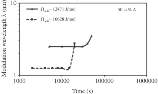
Figure 12 shows the plot of modulation wavelength
λ versus aging time t for B-50at.%A alloy aged at 650 K for ΩA-B values of 12471 and 16628 J/mol. The modulation wavelength λmin is shorter as ΩA-Bincreases. Besides, the start time is shorter for the phase decomposition with the highest value of ΩA-Bparameter, which can be attributed to a higher driving force. It is important to mention that the kinetic behavior of phase decomposition increases as the aging time increases in Figure 12. This fact can be related to the coarsening stage of the decomposed phases6.
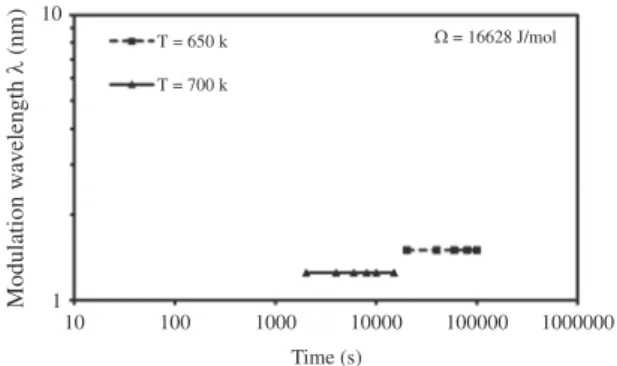
The effect of the aging temperature on the modulation growth kinetics is shown in Figure 13 for B-50at.%A alloy with a ΩA-Bvalue of 16628 J/mol. The increase in the aging temperature caused a lower driving force, see Figure 1; nevertheless, the increase in the atomic mobility, due to the higher atomic diffusion, promoted that the phase decomposition started first at a higher aging temperature.
Figure 10. Microstructural evolution for B-30at.%A alloy for
ΩA-B= 16628 J/mol at 650 K.
Figure 11. Plots of modulation wavelength λ vs. time t for B-30 and 50at.%A alloys for ΩA-B= 16628 J/mol at 650 K.
Figure 12. Plots of modulation wavelength λ vs. time t for B-50at.%A alloy at 650 K for ΩA-B values of 12471 and 16628 J/mol. The minimum modulation wavelength is very close for the two aging temperatures since they have the same interaction parameter.
Figure 14 shows the growth kinetics of spinodal decomposition for the A-50 at.% B alloy with ΩA-B values of 12471 J/mol (1500 R) and 16628 J/mol (2000 R) using both equations at 650 K. In both cases, the modulation wavelength remains almost constant with time, which is also a characteristic of the spinodal decomposition process9. It
is evident that the modulation wavelength λ, is shorter for
Figure 9. Microstructural evolution for B-50at.%A alloy for
the nonlinear equation than for the linear one. In the case of the nonlinear equation, a higher value of ΩA-Bcaused that the start of the phase decomposition growth kinetics was faster. This is attributed to the higher values of the first derivative as ΩA-B increases. A higher first derivative value, or driving force, can be adopted as the reason for the shorter minimum wavelength λmin for spinodal decomposition using the nonlinear equation. The higher values for minimum wavelength λmin in the linear equation seem to be associated with the lower driving force, lower values of second derivative, as explained in section 3.1. Therefore, a longer
aging time is needed to reach the longer wavelength λmin for the start of the spinodal decomposition.
3.4.
Comparison with actual alloy systems
The use of low interaction ΩA-Bparameters causes that the Tc temperature of the miscibility gap to be located at low temperatures, see Equation 4. This promotes a low atomic diffusion which makes the phase decomposition process be very slow. For instance, Cu-Ni alloys12
have a miscibility gap at low temperatures, lower than 573 K and its kinetic behavior of phase decomposition is very slow due to its low atomic diffusion at these temperatures. Furthermore, it has been reported that the phase decomposition takes longer aging times than several years. In contrast, the use of high ΩA-B values makes the Tc temperature be higher which promotes the atomic diffusion and thus the appearance of the phase decomposition. For instance, the phase decomposition in Fe-Cr alloys occurs at higher temperatures6 and the
phase decomposition process is much more rapid than that observed in Cu-Ni alloys. Table 2 shows a comparison of simulated results, the modulation wavelength and morphology of decomposed phases, for the present work using nonlinear equation with other simulated and experimental results for Cu-Ni and Fe-Cr alloys14-17. The
simulation results corresponding to ΩA-B values of 8314 and 12471 J/mol have the Tc temperature of the miscibility gap located at temperatures between 500 and 750 K. This temperature range is close to that of the miscibility gap in Cu-Ni alloys14-15. Furthermore, the minimum value of the
modulation wavelength for the present work is in good agreement with the experimental and calculated values reported in the literature for Cu-Ni alloys. In contrast, the ΩA-B and Tc values of 16628 J/mol are close to those in Fe-Cr alloys. The minimum value of modulation wavelength for the A-B alloy shows a good agreement with those reported in the literature for Fe-Cr alloys16,17.
Finally, the morphology prediction of the decomposed phases corresponds to that reported in the literature.
4. Conclusions
Both linear and nonlinear Cahn-Hilliard equations reproduced the basic characteristics of the morphology and growth kinetics of the spinodal decomposition in the early
Figure 13. Plots of modulation wavelength λ vs. time t for B-50at.%A alloy at 650 K and 700 K for ΩA-B= 16628 J/mol.
Figure 14. Plots of modulation wavelength λ vs. time t for linear and nonlinear equations for ΩA-B values of 12471 and 16628 J/mol.
Table 2. Comparison of present work simulated results with other works.
System Ω (J/mol) TC (K) Calculated
λmin(nm)
Experimental
λmin(nm)
Morphology (Simulation)
Morphology (Experimental)
Cu-Ni[12,15] 8366 573 2 1-2 Irregular and
interconected
Irregular and interconnected
Fe-Cr[16,17] 18600 1100 1-3 2 Irregular and
interconnected
Irregular and interconnected
A-B 8314 500 2-3 --- Irregular and
interconnected
---A-B 12471 750 2-2.5 --- Irregular and
interconnected
---A-B 16628 1000 1-1.5 --- Irregular and
---stages of aging for hypothetical A-B alloys. The increase in the thermodynamic interaction parameter ΩA-B caused a shorter start time for the phase decomposition. The higher aging temperature promoted the faster phase decomposition due to the higher atomic diffusion. The kinetic behavior for the phase decomposition calculated by the linear equation is slower than that of the nonlinear one which can be attributed to the difference in the driving force parameter of each
equation. The microstructure evolution and kinetics of phase decomposition of
Cu-Ni and Fe-Cr alloys showed a good agreement with the present work results.
Acknowledgements
The authors wish to acknowledge the financial support from SIP-IPN-CONACYT 100584.
References
1. Janssens KGF, Raabe D, Kozeschnik E, Miodownik MA and Nestler B. Computational Materials Engineering. 1st ed. Elsevier Academic Press; 2007.
2. Avila-Davila EO, Melo-Maximo DV, Lopez-Hirata VM, Soriano-Vargas O, Saucedo-Muñoz ML and Gonzalez-Velazquez JL. Microstructural simulation in spinodally-decomposed Cu-70at.%Ni and Cu-46at.%Ni-4at.%Fe alloys.
Materials Characterization. 2009; 60:560-567. http://dx.doi. org/10.1016/j.matchar.2009.01.003
3. Montaño-Zuñiga IM, Sepulveda-Cervantes G, Lopez-Hirata VM, Rivas-Lopez DI and Gonzalez-Velazquez JL. Numerical simulation of recrystallization In bcc metals.
Computational Materials Science. 2010; 49:512-517. http:// dx.doi.org/10.1016/j.commatsci.2010.05.042
4. Rapaz M, Bellete M and Deville M. Materials Modelling in Materials Science and Engineering. 1st ed. Berlin: Springer-Verlag; 2010.
5. Chen LQ. Phase Field Modeling of Materials Microstructure. In: Xiao Guo Z, editor. Multiscale materials modeling.
C R C P r e s s L L C ; 2 0 0 7 . p . 6 2 - 8 3 . h t t p : / / d x . d o i . org/10.1533/9781845693374.62
6. Honjo M and Saito Y. Numerical simulation of phase separation in Fe-Cr binary and Fe-Cr-Mo ternary alloys with use of the Cahn-Hilliard equation. ISIJ International. 2000; 40:914-919. http://dx.doi.org/10.2355/isijinternational.40.914
7. Kim SG and Kim WT. Phase field modeling of solidification. In: Yip S, editor. Handbook of Materials Modeling. Netherlands: Springer; 2005. p. 2106-2116.
8. Kostorz G. Phasetransformations in Materials. 2nd ed. Wiley-VCH; 2001. PMid:11505305. http://dx.doi. org/10.1002/352760264X
9. Hilliard JE. Spinodal Decomposition. In: Aaronson HI, editor. Phase transformations. Metals Park Ohio ASM; 1970. p. 497-560.
10. Cahn JW. Spinodal decomposition. Transactions of the Metallurgical Society of AIME. 1970; 242:89-103.
11. Avila-Davila EO, Lezama-Alvarez S, Saucedo-Muñoz ML, Lopez Hirata VM and Gonzalez-Velazquez JL. Numerical simulation of the spinodal decomposition in hypothetical A-B and A-B-C alloy systems. Revista de Metalurgia, 2012; 48:223-236. 12. Chen LQ. Computer Simulation of Spinodal Decomposition
in Ternary Systems. Acta Metal Mater. 1994; 42:3503-3513. http://dx.doi.org/10.1016/0956-7151(94)90482-0
13. Nishizawa T. Thermodynamics of Microstructure. 1st ed. ASM International; 2008.
14. Lopez-Hirata VM, Sakurai T and Hirano K. A study of phase separation in Cu-Ni alloys by AP-FIM. Scripta Metallurgica et Materialia. 1992; 26:99-103. http://dx.doi.org/10.1016/0956-716X(92)90377-Q
15. Avila-Davila EO, Lopez Hirata VM, Saucedo-Muñoz ML and Gonzalez-Velazquez JL. Microstructural simulation of phase decomposition in Cu-Ni alloys. Journal of Alloys and Compounds. 2008: 460:206-212. http://dx.doi.org/10.1016/j. jallcom.2007.05.070
16. Soriano-Vargas O Avila-Davila EO, Lopez Hirata VM, Saucedo-Muñoz ML, Cayetano-Castro N and Gonzalez-Velazquez JL. Effect of spinodal decomposition on The mechanical behavior of Fe-Cr alloys. Materials Science and Engineering: A. 2010; 527:2910-2914. http://dx.doi. org/10.1016/j.msea.2010.01.020
17. Lopez Hirata VM, Soriano-Vargas O, Dorantes-Rosales HJ and Saucedo-Muñoz ML. Phase decomposition in an Fe-40at.%Cr alloy after isothermal aging and its effect on hardening.