doi: 10.1590/0101-7438.2016.036.01.0023
ALTERNATIVE METHODS TO MULTIPLE CORRESPONDENCE ANALYSIS IN RECONSTRUCTING THE RELEVANT INFORMATION IN A BURT’S TABLE
Sergio Camiz
1and Gast˜ao Coelho Gomes
2*Received September 11, 2015 / Accepted February 20, 2016
ABSTRACT.In this work, the reconstruction of the Burt’s table, Greenacre (1988)’s Joint Correspondence Analysis (JCA), and Gower & Hand (1996)’s Extended Matching Coefficient (EMC) are compared to Mul-tiple Correspondence Analysis (MCA) in order to check the quality of the methods. In particular, for the whole table, the ability is considered separately the diagonal, and the off-diagonal tables, that is the abil-ity to describe either each character’s distribution or the interaction between pairs of characters, or both. The theoretical aspects are discussed first, and finally the results obtained in an application are shown and discussed.
Keywords: Correspondence Analysis, Multiple Correspondence Analysis, Joint Correspondence Analysis, Extended Matching Coefficient, Singular Value Decomposition.
1 INTRODUCTION
Both Multicriteria Analysis and Multicriteria Decision Models [4, 37] are tools largely adopted in operational research, in particular when dealing with Knowledge Discovering in Databases [14]. In present days it may be of high interest to deal with qualitative unstructured data, whose treatment may be more complex. Studies in this framework are found in recent operational re-search literature [16, 17, 30, 40]. In this context, data reduction through exploratory multidimen-sional scaling may contribute to clarify the data at hand, by revealing structures and factors. In particular, factors, together with the observed characters most associated to them, may lead to a consistent dimension reduction and at the same time to the ability to select the most appropriate characters to take into account for further, more focused investigation. Thus, the identification of the proper dimension of a data table may be a topic of investigationper se.
In exploratory multidimensional scaling the identification of the proper dimension of the solution is the basis to define a threshold between relevant information and residuals. The relevant infor-mation is also tied to the possibility of interpreting the factors according to the paradigms of the
*Corresponding author.
1Dipartimento di Matematica, Sapienza Universit`a di Roma, Italy. E-mail: [email protected]
methods at hand: in the linear case, the percentage of explained inertia is the most widely used. Thus, to take into account a large share of inertia is the most evident rough method that may be used and a higher-dimensional solution is normally preferred rather than a smaller one only if its corresponding inertia is significantly larger than a smaller-dimensional solution. Tied to this aspect, the reconstruction of the original data table according to a lower rank matrix is of rele-vance, since a good reconstruction of the data obtained this way is helpful to better understand to what extent the reduction in dimension, through the use of factors, is a reasonable approximation of the original data.
In this paper, we consider the special case of qualitative data, that are usually summarized by the so-called Burt’s matrix, the super-contingency table that cross-tabulates all characters taken into account. Multiple Correspondence Analysis (MCA) [7, 19] is the best known exploratory factor analysis method to deal with it, but alternative methods are proposed in literature, based on different rationale. Critics toMCAemphasize the misuse of the chi-square metrics [18], a metrics that for contingency tables finds its rationale in the partition of the chi-square in inde-pendent components [27, 35, 44], thus on the deviation from the expectation. Now, to compute distances between lines in both the indicator matrix and its square, the Burt’s table, such met-rics is tremendously biased by the obvious (squared) differences between levels belonging to the same character [20, 21]. In addition, rare levels raise their importance in the computation but en-hance aspects that reveal being useless, since the chi-square statistics may not be applied to these tables; hence, its use is hardly justifiable [18]. Eventually, it is known since long the problem of the underestimation of the inertia explained by the factors, that deserve being re-evaluated in some way [2, 8, 19]. Indeed, applying the chi-square metrics to such a table, the highest contribu-tions to the total inertia result from the block-diagonal tables crossing each character with itself, which is information without noticeable value, since this way the expected values provide the maximum deviation from expectation. Along with this, a problem results in the unpredictabil-ity of the partial data reconstruction of the Burt’s table, as already put in evidence by [10]. The problem may be relevant in qualitative discriminant analysis [39], which is based onMCA coor-dinates. Here, a bad reconstruction would prevent the reduction of the number of factors to take into account.
Correspondence Analysis to the simultaneous analysis of several 2-way contingency tables. The idea is analogous to the one of [42] to fit the off-diagonal elements of a correlation matrix and is obtained by numerical optimization. Therefore, this time different dimensional solutions are not encapsulated.
To compare the results, we consider the reconstruction quality only. At the end, these methods will be applied to a very small table, taken from studies in linguistics [32].
2 THEORETICAL FRAMEWORK 2.1 Singular Value Decomposition
We may ground our further discussion on the well-known Singular Value Decomposition (SVD, [1, 19]) theorem, which states
Theorem 1. Any real matrix X may be decomposed as X = U1/2V′, withthe diagonal matrix of the real non-negative eigenvalues of X X′, U the orthogonal matrix of the correspond-ing eigenvectors, and V the matrix of eigenvectors of X′X (with the same eigenvalues), with both constraints U′U =I and V′V =I .
This theorem corresponds to the reconstruction formula of anS-rank matrixX∈Rr×c
xi j = S
α=1
λα uiα vjα, ∀i ∈(1,r),j ∈(1,c) (1)
or, in vector notation
X =
S
α=1
λα uαv′α,
on which the Eckart & Young’s theorem [13] is based:
Theorem 2.(Eckart and Young) The s-rank reconstruction of any real matrix X , with s<S, the rank of X , once its singular values are sorted in decreasing order,
X≈
s
α=1
λα uα v′α=H
is the best one in the least-squares sense.
This means that, for everys < S, the matrixHssolves the problem to approximate a matrixX
by another matrixHof lower rank at the best in the least-squares sense, thus by minimizing
r
i=1
c
j=1
(xi j−hi j)2=trace
(X−H)(X−H)′ (2)
As it is trivial that trace(HsHs′)=
s
α=1λα,the minimum of (2) reached byHsequals
trace(X−Hs)(X −Hs)′
=
S
It is well-known that Principal Component Analysis (PCA,[26]) finds its rationale in this theo-rem, once the data table is standardized according tozi j = x√i jn− ¯σxj
j , withx¯j andσj the average
and the standard deviation of thej-th character; indeed, this wayZ′Z =cor(X)=C, the matrix of correlations between the columns ofX. Thus, given thePCAof the correlation matrixC, with andV as their diagonal matrix of eigenvalues and unit matrix of eigenvectors respectively, and givenU as the unit eigenvectors ofZ Z′, the reconstruction formula (1) becomes
xi j =
r
α=1
λα uiα vjα √nσj+ ¯xj, ∀i ∈(1,r),j ∈(1,c) (3)
For correspondence analysis, we shall adopt the Generalized Singular Values Decomposition (GSVD, [1, 19]), in which two other matrices are involved:
Theorem 3. Given two real positive definite matrices M and N , any real matrix X may be decomposed as X =U1/2V′, under constraintsU′MU=I andV′NV =I.
The solution is given by theSV Dof the matrixX =M1/2X N1/2= F1/2G′, withF′F= I,
G′G = I,U = M−1/2F, andV = N−1/2G. It results thatUU′ = M−1 andVV′ = N−1 respectively.
In this case the minimization problem (2) becomes
r
i=1
c
j=1
(x˜i j− ˜hi j)2=trace
(
X−H)( X−H)′
withH=sα=1√λα ˜fα g˜′α,withs≤S=rank(X).
Using the matrix
Hs =M−1/2 HN−1/2= s
α=1
λα (M−1/2f˜α) (N−1/2g˜α)′, (4)
as trace(HH′)=sα=1λα,the minimization problem is solved as:
r
l=1
c
k=1 ⎛ ⎝
r
i=1
c
j=1
m1/2li (xi j− ˆhi j)2n1/2j k
⎞ ⎠ 2
=traceM(X−Hs)N(X −Hs)′
=
S
α=s+1 λα. (5)
In the particular case in which bothM andNare diagonal, (5) simplifies to
r
i=1
c
j=1
mii nj j(xi j − ˆhi j)2=trace
M(X−Hs)N(X−Hs)′
=
S
α=s+1
λα. (6)
among them, that is to identify at least a tentative cutpoint of either the singular- or the eigen-values sequence, remains a crucial issue, that did not find a univocal solution so far (forPCA see, e.g., [11, 25, 36]). In Simple Correspondence Analysis (SCA, [7, 19]), it seems more eas-ily solved, since the special chi-square metrics adopted allows a useful solution and an easy interpretation of the results, and regardingMCAwe shall see that [5, 6] propose an interesting method.
2.2 Simple Correspondence Analysis
Let N an r ×ccontingency table, withn = n.. the table grand total, X = N/n the table of relative frequencies pi j = ni j/n, r = (p1., . . . ,pr.)′ the vector of row marginal profile, c=(p.1, . . . ,p.c)′the vector of column marginal profile, and Dr =diag(r),Dc =diag(c)the
corresponding diagonal matrices. LetE =rc′represents the table with equal marginal profiles ofXunder the independence hypothesis. TheSCAofNresults from the application ofGSVDto the matrixX with the real positive definite matrices represented by the diagonal matricesDr−1 and D−c1. In this particular case the decomposition results X = Dr−1/2X Dc−1/2 = F1/2G′
and both matrices XX′ and X′X have a trivial eigenvalueλ1 = 1 to which the eigenvectors ˜
f1 =(√ri)andg˜1 =(√cj)correspond respectively. It can also be shown that the other
non-trivial eigenvalues are always contained between 0 and 1. If we take off the summation the non-trivial eigenvalue, thes-rank reconstruction formula(s≤S=min(r,c))may be little transformed:
pi j≈ ˆhi j,s = ricj s
α=1
λα(ri1/2 f˜iα) (c1/2j g˜jα)
= ricj
1+
s
α=2
λα(ri−1/2 f˜iα) (c−j1/2g˜jα)
(7)
Incidentally, we observe that, in order to produce graphics with simultaneous symmetrical rep-resentation of both rows and columns, theSCAeigenvectors are usually rescaled by defining as coordinates the vectorsϕα andψα given byϕiα =λ
1/2 α r−
1/2
i f˜iα andψjα = λ 1/2 α c−
1/2
j g˜jα, respectively. In this case the reconstruction formula (7) becomes
pi j ≈ ˆhi j,s =ricj
1+
s
α=2 1 √
λα
ϕiαψjα .
Thus, depending on which coordinates one chooses, the reconstruction formula forNbecomes:
N =nr c′+n DrF1/2G′Dc=nr c′+n Dr−1/2 ′Dc. (8)
Returning to the optimization problem (6), we may explicitly write the residual as
traceDr−1(X −Hs)Dc−1(X−Hs)′
=
r
i=1
c
j=1
(xi j − ˆhi j,s)2
ri cj = S
α=s+1
Now, if we consider the 1-rank reconstruction, that is Hˆ1 = E = rc′, the residual takes the particular form
r
i=1
c
j=1
(xi j− ˆhi j,1)2 ri cj =
r
i=1
c
j=1
(xi j−ri cj)2
ri cj = S
α=2
λα. (10)
that is the sum of squared deviations of the observed values from the expected ones under inde-pendence divided by the expected ones. This is commonly called theinertiaof the tableX that is, up to the factorn, the chi-square ofN; indeed, multiplying (10) byn, we get
n
r
i=1
c
j=1
(pi j− ri cj)2
ri cj = r
i=1
c
j=1
(ni j −n ri cj)2
n ri cj =
χ2=n
S
α=2
λα. (11)
Hence, the decomposition of the inertia along the non-trivial eigenvectors ofSC Aleads to the decomposition of the chi-square along each corresponding dimension:
χ2=n(λ2+ · · · +λS)=χ22+ · · · +χS2
αequalsχα2=nλα.
Based on [44], this result led [35] to check for significance the partial chi-squares associated to each eigenvalue,χα2withd f =(r+c−2α−1)degrees of freedom, to detect if there are linear ordinations of both rows and column levels that explain the deviation from expectation. Indeed, [28] proved that the first eigenvalue is larger than the corresponding chi-square and [29] proved that the distribution of the eigenvalues is that of those of a Wishart matrix(W(m1−1)(m2− 1),Min(m1−1,m2−1),I). Nevertheless, [15] finds that the sum of the smallest eigenvalues may be used as a test for their nullity, that leads to the Malinvaud’s [31] stopping rule, to test the residuals of each reduced rank solution. Indeed, one may test for significance
Qs =
i j
ni j −nhˆi j,s
2
nricj =
χ2−
s
α=2 χα2=n
S
β=s+1 λβ,
asymptotically chi-square-distributed with(r−α−1)×(c−α−1)degrees of freedom.
2.3 Multiple Correspondence Analysis
Let us consider now a qualitative data tableX withnobservations, withQas nominal characters and J as the total number of levels, that is J = iQ=1li, whereli is the number of levels of
thei-th character. It is well-known thatMCAof such a matrix is nothing but a generalization of SCAand it is based onSCAof either the indicator matrixZ, whose rows are the units and the columns are all theJlevels of theQconsidered variables, or the so-called Burt’s tableB=Z′Z that gathers all contingency tables obtained by cross-tabulating all the variables inZ, including the diagonal tables obtained by crossing each variable with itself. The idea is to adopt for both matrices the same optimized decomposition ofSCA, namely theGSVDof eitherQ−1Z Dr−1or
Indeed, it is evident that the latter is the square of the previous, so that they share the eigenvectors, and the singular values in Burt’s case are the squares of those of the indicator matrix case:να= µ2α. The identity of the eigenvalues allows identical interpretation of the resulting factors. Thus, it makes no difference to performMCAon either matrix. On the other side, whereas the total inertia of Z is Iz = J−QQ, the one of B equalsνα = µ2α. In both cases, the chi-square metrics is adopted so that the interpretation of results ought to be done once again in terms of deviations from expectation. This point deserves some special attention, since the deviation refers to all contingency tables gathered in the Burt’s table, including the diagonal ones. The problem is that such diagonal matrices, that “theoretically” would indicate maximum deviation, in this case are just the expected ones, as they cross each character with itself.
AsSCA, given a Burt matrixB,MCAmay be defined as the weighted least-squares approxima-tion ofBby another matrixHof lower rank, minimizing
n−1Q−2traceDr−1(B−H)Dr−1(B−H)′. (13)
Notice how (13) derives from (10). In terms of the subtables, this may be rewritten as
n−1Q−2traceD−1(B−H)D−1(B−H)′=
=n−1
Q
i=1
Q
j=1
traceDi−1(Ni j−Hi j)D−j1(Ni j−Hi j)′
,
whereHis the supermatrix of theHi j. Introducing the norm notation
A−B2i j =trace
Di−1(A−B)D−j1(A−B)′
the minimization can be written as
n−1
Q
i=1
Q
j=1
Ni j−Hi j
2
i j. (14)
InMCAthe identification of the true dimension is particularly difficult, despite the MCAis a SCAof a particular table, because the chi-square test has no sense. Indeed, forB a chi-squared statistic may again be calculated as if it were a contingency table, and this simplifies as
χ2B =2
Q
i=1
i−1
j=1
χi j2 +n(J−Q),
whereχi j2 is the chi-squared statistic for the off-diagonal subtableNi j = Zi′Zj crossing thei-th
and the j-th characters, but without the possibility to make a test. Unfortunately neitherQαnor
The high number of eigenvalues of theMCA, and their corresponding low values, were criticized by the same Benz´ecri [8] that suggests to reevaluate those larger than their average. Indeed, applying bothSCAandMCAto the same two characters, by partitioning the Burt’s table Z′Z into submatrices it can be shown (ibid.) the relationµα = 1±
√
λα
2 that holds amongµα, the eigenvalues ofZ, andλα, those of theSCAof the contingency table crossing the two characters. In this case, it is evident that to the eigenvaluesλα =0 ofSCAcorrespond eigenvaluesµα = 12 of Z andνα = 14 of B, whereas to the other two correspond, one of which larger and the other smaller than 12and14respectively. To generalize this argument to several characters results in admitting to limit attention in MCAonly to the eigenvalues larger than their mean, that is µ≥µα= Q1.
The argument is discussed in detail by both Benz´ecri [8] and Greenacre [20, 21]. Both authors suggest, in order to get a measure of relative importance of each factor, to re-evaluate the eigen-values larger than the mean (equal to Q1) according to the formula
ρ (µα)=
Q
Q−1 2
(µα−µ)2, µα ≥µ= 1 Q.
Benz´ecri [8] suggests to consider as total inertia the sum of the re-evaluated eigenvalues and to take as percentage of explained inertia the ratio ρ(µα)
αρ(µα). This results in a dramatic re-evaluation of the relative importance of the first eigenvalues. On the opposite, Greenacre [20] bases his arguments on the unusefulness to take into account the diagonal block matrices and the utility to limit attention only to the total off-diagonal inertia of the table, that is the sum of squared (non-re-evaluated) eigenvalues minus the diagonal inertia; represented as:
Q
Q−1 ⎛
⎝
µα>1/Q
µ2α − J−Q Q2
⎞ ⎠.
Experiments show that the Greenacre’s reevaluation is always limited to a share of the total iner-tia of Burt’s table even by taking into consideration all the eigenvalues larger than the mean. This does not affect the interpretation of the factors, that essentially depends upon the eigenvectors – and thus to the contributions of both levels and characters to them –, but affects more the quality of representation of these elements on the factor subspaces, that varies according to the percent-age of inertia attributed to each one. Indeed, this is a point that would deserve some specific consideration, in particular in deciding which reevaluation may be better taken into account. In the following, we shall call adjusted MCAthe one with re-evaluated inertia, therefore with the coordinates recalculated accordingly.
The reduction in number of the dimension, thanks to both Benz´ecri’s and Greenacre’s reevalua-tions, does not solve the problem of the true dimension of the table. To this question, an answer comes from Ben Ammou & Saporta [5, 6]: they suggest to estimate the significance of the eigen-values ofMCAaccording to their distribution. If the characters are independent,
J−Q
β=1 µβ =
J−Q
Q and Sµ2 =
J−Q
β=1
µ2β = J−Q Q2 +
i=jφi j2
withn..φi j2 ≈χ(2li−1)(lj−1), thus,
E[n..φi j2] =E[χi j2] =(li −1)(lj −1)
so the expectation of the varianceS2µof the eigenvalues is
σ2=E[Sµ] =2 1 n..Q2(J−Q)
i=j
(li−1)(lj −1).
Roughly, one may assume that the intervalQ1 ±2σshould contain about 95% of the eigenvalues. Indeed, since the kurtosis of the set of eigenvalues is lower than for a normal distribution, the actual proportion is larger than 95%.
2.4 Joint Correspondence Analysis
Greenacre [20] criticizes theMCAapproach, stating that it is not a natural generalization ofSCA, and proposes as more natural hisJoint Correspondence Analysis(JCA). With it, he overcomes theMCA’s useless fitting of the diagonal subtables ofBwhich contribute with the termn(J−Q) to the total inertia. Hence, he takes as more natural measure of total inertia the sum q=sχqs2 of the inertias of the off-diagonal tables. This suggests an alternative generalization of correspon-dence analysis which fits only the off-diagonal tables, analogous to factor analysis where values on the diagonal of the covariance or correlation matrix are of no direct interest.
Indeed, the proposed redefinition of the total inertia, by removing the diagonal block-matrices, would fix an important bias due to the application to the Burt’s table of the chi-square metrics, since the diagonal structure of the diagonal block-matrices represents a very high fictitious devi-ation from the expected values, thatMCAanalyzes as if it were a true deviation. On this basis, opposite to the current use, this kind of analysis is not really suitable.
Greenacre [20] proposes hisJoint Correspondence Analysis(JCA) as a weighed least-squares approximation aiming at minimizing
n−1
Q
i=1
i−1
j=1
Ni j−Hi j
2
i j, (15)
instead of (14) with the correspondingχ2J = iQ=1ij−=11χi j2, sum of the chi-squares of all off-diagonal tables, that unfortunately may not be checked for significance.
In order to get the solution, he proposes an alternating least-squares algorithm, based on the reformulation of (15) as follows:
n−1
Q
i=1
i−1
j=1
Ni j−Hi j
2
i j =n−
1
Q
i=1
i−1
j=1
Ni j−nrirj′−Li j
2
i j (16)
withri the diagonal of thei-th block-diagonal matrix. CallingH andLthe supermatrices
satisfies the normal equations in the minimization of the second term of (16) with the rank-(K+1)matrixH =r r′+Lwhich satisfies minimizing (15), withrthe supervector gathering theQvectorsri.
The matrix approximationLof rankKis of the formL =n D X DβX′D, where theJ×Kmatrix X is normalized as X′D X = Q I, with D = diag(r). The matrix X of parameters has rows corresponding to the categories of the variables and columns corresponding to the dimensions of the solution, that must be chosen in advance. The diagonal matrixDβcontains a scale parameter for each dimension. This form of L and the normalization conditions are chosen to generalize the bivariate case (8). The parameter matrixX is partitioned row-wise according to the variables as X1, . . . ,XQ, where Xqis Jq×K, so that the submatrices ofL areLqs=n DqXqDβXs′Ds.
There are also inherent centering constraints onX of the formX′r=0 due to the orthogonality with the dimension defined by the trivial solution. It is evident that the dimension of the solution must be chosen in advance.
Thus [20] proposes the approximate reconstruction of the whole matrixB−nr r′, namely
B−nr r′≈n D X DβX′D+C,
whereCis a block diagonal matrix with submatricesCqq, q = 1, . . . ,Qdown the diagonal
and zeros elsewhere. Here, eachCqqis composed by dummy parameters which effectively allow
perfect fitting of the submatrices on the diagonal ofB−nr r′, thereby eliminating their influence on the model of interest. The minimization of
B−nr r′=2n−1
Q
i=1
i−1
j=1
Ni j−nri rj ′−Li j
2
i j
+ n−1
Q
k=1
Nkk−nrkrk′−Lkk −Ckk
2
k.
(17)
is equivalent to minimizing (16) because the latter set of terms in (17) can always be made zero by settingCii =Nii −nri ri ′−Lii.
The algorithm proposed by [20] to minimize (17) can be performed iteratively by alternating between the variables inCand those inXandDβ as follows:
1. fix the dimensionK of the solution.
2. initiate the algorithm with an analysis of the full Burt matrixB, that is
B−nr r′≈n D X DβX′D. (18)
3. limiting attention to the firstK dimensions, say the firstK columns ofX x(1), . . . ,x(K), (18) can be rewritten as
B−nr r′≈
K
k=1
so that, if all quantities except theβk(k = 1, . . . ,K)are regarded as fixed, the problem
reduces to a simple weighted least-squares regression (see [20], for further details).
4. KeepingX andDβ fixed, set
Cii =Nii −nri ri ′−n DiXiDβXi′Di (i=1, . . . ,Q).
5. KeepingC fixed, minimize with respect to X andDβ: this is achieved by performing a correspondence analysis on the tableB∗ =B−C, that is the Burt’s matrix with modified submatrices on its diagonal, settingXequal to the firstKvectors of optimal row or column parameters and the diagonal ofDβequal to the square roots of the firstKprincipal inertias respectively.
6. Iterate the last two steps until convergence.
In the special caseQ=2, the problem reduces to fitting the single off-diagonal submatrixN12. It is relevant to mention that the initial solution described above is optimal and provides the simple correspondence analysis of N = N12 exactly. It is also noteworthy to quote [22, pag. 148]’s alternative proposal to reevaluate the inertias along the axes by estimating them through a weighted least-squares regression. Indeed, it means to estimate only once theβks in (19), where
thexks are the eigenvectors issued byMCA, once the dimension of the solution K is decided.
We are not convinced by this solution, since the objections that concern the use of the chi-square metrics remain unaltered.
2.5 The Extended Matching Coefficient
JCAwas introduced by [20] as a way to drop the excessive attention given to the diagonal of the Burt’s matrix byMCA, that indeed does not deserve any interest, but with a different optimization aim, that is to reconstruct at the best the off-diagonal subtables. In this case, the chi-square metrics is justified, whereas we have already stated that in classicalMCAit has no theoretical justification. For this reason, we are not convinced that some inertia reevaluation ofMCA, as the quoted ones, may be a solution. On the opposite, we find interesting to explore Gower & Hand’s [18] proposal to drop the chi-square metrics in favor of a more simple one: theExtended Matching Coefficient. Indeed, for two units, they define it as the number of common levels across all characters. Therefore, given the indicator matrixZ,Z Z′would give us a similarity matrix to deal with; indeed, given its size, the Burt’s tableBas suchisits corresponding in the dual space, so that it is sufficient to perform theSVDof the centered Burt’s matrix, that is
Q−2B=Q−2Z′Z (20)
3 AN APPLICATION TO THE KIND OF WORDS
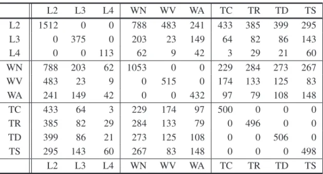
To show in detail the different behavior of the different analyses in practice, we refer first to a data set taken from [32], consisting in 2000 words taken from four different kind of periodic reviews (Childish (TC), Review (TR), Dissemination (TD),andScientific Summary (TS)), classi-fied according to their grammatical kind (Verb (WV), Noun (WN),andAdjective (WA)) and the number of internal layers (Two- (L2), Three- (L3),andFour and more layers (L4)), as a measure of the word complexity. In Table 1 the Burt’s table that results by crossing the three characters is reported.
Table 1–Burt’s table of the words’ type example.
L2 L3 L4 WN WV WA TC TR TD TS
L2 1512 0 0 788 483 241 433 385 399 295
L3 0 375 0 203 23 149 64 82 86 143
L4 0 0 113 62 9 42 3 29 21 60
WN 788 203 62 1053 0 0 229 284 273 267
WV 483 23 9 0 515 0 174 133 125 83
WA 241 149 42 0 0 432 97 79 108 148
TC 433 64 3 229 174 97 500 0 0 0
TR 385 82 29 284 133 79 0 496 0 0
TD 399 86 21 273 125 108 0 0 506 0
TS 295 143 60 267 83 148 0 0 0 498
L2 L3 L4 WN WV WA TC TR TD TS
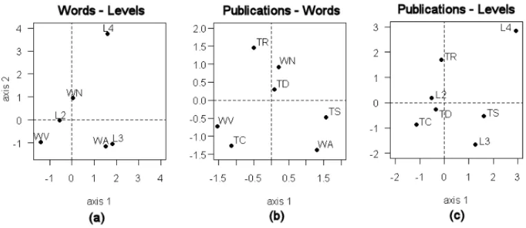
In Table 2 are reported the eigenvalues of the three SCAs of the contingency data tables that cross the three characters two by two: the eigenvalues, the percentage of corresponding inertia, and the p-value associated to the chi-square calculated for the corresponding one-dimensional reconstruction, that, in this case, is identical to the Malinvaud’s test, since each solution is 2-dimensional.
Table 2–SCAof the three contingency data tables of the three characters two by two. In the columns, the eigenvalues, the percentage of inertia, and thep-value of the chi-square associated to the factors.
Words - Levels Publications - Words Publications - Levels
N. Eigen % p-value Eigen % p-value Eigen % p-value
1 .0925 99.98 .0000 .0253 80.53 .0000 .0619 98.82 .0000
2 .0000 0.02 .8625 .0061 19.47 .0022 .0007 1.18 .4771
In Figure 1 the results of the threeSCAs are represented too: it must be pointed out that the vertical position of the items is significant only for the second graphic. Indeed, the inspection of this factor plane shows an arch pattern due to a Guttman effect [9, 24]; the same, the interpre-tation is straightforward: for the first table, both verbs and nouns seem to have in general less syllables than the adjectives; for the second, the variation in use of the words according to the higher complexity of the publication: verbs for the childish, nouns for reviews and dissemina-tions, adjectives for scientific summaries; for the third, the more complicated words (3 and more syllables) in scientific summaries than in all others. It is noteworthy in the second table the oppo-site pattern of verbs and adjectives, the first reducing while the publication is of higher level and the second raising; this explains clearly the observed Guttman effect. The position of long words very elongated on the second axis of both the first and the third analyses, in the latter case also with review is explained by the shortness of the verbs and its scarce presence in childish publi-cations, but it is not significant. We may ground our comparisons on this interpretation of the data. RunningMCA, the pattern of eigenvalues is represented in Table 3, in which are reported the singular values ofZ, their percentage to their total (that equals J−QQ =2.33), the cumulate percentage, the eigenvalues of the Burt’s matrix, corresponding to the explained inertia, and the cumulate inertia.
Figure 1–Words’ type example: The pair of characters levels on the three two-waySCAs: (a) Words vs. Levels; (b) Publications vs. Words; (c) Publications vs. Levels.
Table 3–MCAsingular values, percentage to the total and cumulate percentage, eigenvalues, and cumulate inertia of the Burt’s table of words’ type example. Then re-evaluated inertia and
percent-ages according to both [8] and [20].
N Sing. % Cumul. Eigen. Cum. Re-ev. Benz´ecri’s Greenacre’s
value Inertia % inertia Inertia % Cum.% % Cum.%
1 0.4896 20.98 20.98 0.2397 0.2397 0.0549 95.91 95.91 88.36 88.36 2 0.3640 15.60 36.58 0.1325 0.3722 0.0021 3.69 99.60 3.40 91.76 3 0.3434 14.72 51.30 0.1179 0.4901 0.0002 0.40 100.00 0.37 92.13 4 0.3300 14.14 65.44 0.1089 0.5990 0.0572 100.00 92.13 5 0.3084 13.22 78.66 0.0951 0.6941
6 0.2728 11.69 90.35 0.0744 0.7685 7 0.2252 9.65 100.00 0.0507 0.8192
In Figure 2athe distribution of all character levels on the plane spanned by the first two factors of MCAis represented. Indeed, the patterns of all the characters’ levels repeat fairy well the same in the three two-way tables: thus it may be taken as a sign of coherence between the individual SCAs andMCA.
Figure 2–Words’ type example: representation of the three-character levels on the plane spanned by the
first two factors: (a)MCA; (b)JCA.
Let us now discuss the results of theJCAcarried out on the same example. In the 2-dimensional solution1the axes inertias are 0.2488 and 0.0272, with a proportion of 90.15% and 9.85%, re-spectively: considering only the first axis as significant, we may observe in Figure 2ba pattern of levels nearly identical to the one ofMCA. Some differences appear on the second axis, in which are noticeable the very different positions of verbs and childish publications on the negative side and of long words and summaries on the positive one, but, once again, this may not be considered significant.
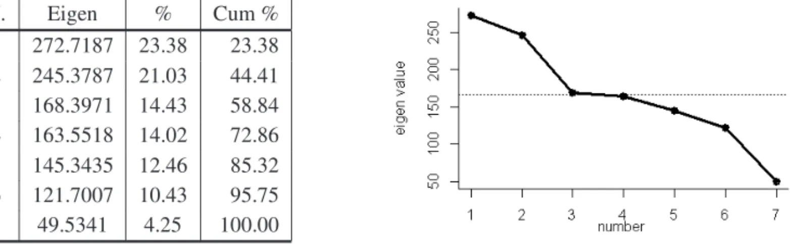
Table 4–Eigenvalues, percentages of explained and cumulate inertia of the analysis ofEMCon Words’ type example. On the right, the pattern of the eigenvalues. The dotted line represents their average (166.66).
N. Eigen % Cum %
1 272.7187 23.38 23.38 2 245.3787 21.03 44.41 3 168.3971 14.43 58.84 4 163.5518 14.02 72.86 5 145.3435 12.46 85.32 6 121.7007 10.43 95.75 7 49.5341 4.25 100.00
Eventually, we got the results ofEMC. The seven(J−Q)non-zero eigenvalues and the cor-responding percentages of explained and cumulate inertia are reported on Table 4. They are reported also in the figure nearby, where the average (166.66) corresponds to the dotted line. Thus, one may identify two major eigenvalues that summarize 44% of the total inertia, three others around the mean and two minor ones. Here, the Cattel test would suggest two factors, whereas the brokenstick considers random even the first one, since the threshold to consider it non-random would be 37.04%. These contradictory results lead us to compare them with the previous ones, therefore considering the first dimension as the “true” one, but also taking into account the second, at least for the graphical representation. In Figure 3 all levels are plotted on the plane spanned by the first two factors: indeed, the pattern of levels along the first axis is somehow similar to the ones resulting from bothMCAandJCAbut not so much: bothL4andL3 and even moreWAandWNare exchanged, slightly modifying the interpretation of the results. On the opposite, the pattern along the second factor is so different that no agreement seems to be possible. In both cases, differences may result from the fact that here rare levels are found close to the centroid and the frequent ones are far away, whereas in the chi-square-based methods the opposite occurs. Indeed, this is the case of bothL2andWNthat have the highest marginal values, whereasL4, with the lowest ones, is set toward the center.
Let us look now at the one-dimensional reconstruction, as resulting by theSCAs of the three individual tables, by theMCA, and by Greenacre’sJCAas reported in Table 5. The comparison of the SCAone-dimensional solutions with the original tables shows that the amount of the
Figure 3– Words’ type example: representation of the three-character levels on the plane spanned by
the first two factors of the centeredPCAon the Burt’s table, corresponding to the Extended Matching Coefficient.
cumulate absolute residuals is in good agreement with the quality of the solution, as represented by the corresponding chi-square. For this reason, the low quality of the reconstruction of the table crossing kind of words with the type of publications depends on the significance of the second dimension of theSCAof this table, that here is not taken into account. At first glance, it is evident the high difference in the cumulate absolute residuals ofMCAin respect to the other solutions, that is an important sign of the limits ofMCAin respect toJCA.
Table 5–Original two-way contingency tables of words’ type example and their
reconstruc-tion according to the first dimension ofSCAs,MCA, adjustedMCA,JCA, andEMCwith the corresponding cumulate absolute residuals.
Original Contingency Tables
WN WV WA TC TR TD TS TC TR TD TS
L2 788 483 241 L2 433 385 399 295 WN 229 284 273 267
L3 203 23 149 L3 64 82 86 143 WV 174 133 125 83
L4 62 9 42 L4 3 29 21 60 WA 97 79 108 148
SCAFirst Layer
WN WV WA TC TR TD TS TC TR TD TS
L2 788 483 241 L2 435 382 400 296 WN 253 257 267 276
L3 204 23 149 L3 60 89 85 141 WV 165 144 127 79
L4 61 9 42 L4 5 25 22 61 WA 82 96 112 142
SCAcumulate absolute residuals
2 29 134
MCAFirst Layer
WN WV WA TC TR TD TS TC TR TD TS
L2 770 559 183 L2 492 409 401 211 WN 249 257 264 283
L3 216 -24 183 L3 13 69 82 211 WV 219 155 145 -3
L4 67 -20 66 L4 -5 18 23 76 WA 32 84 97 219
MCAcumulate absolute residuals
304 342 397
AdjustedMCAFirst Layer
WN WV WA TC TR TD TS TC TR TD TS
L2 783 471 258 L2 433 385 399 295 WN 229 284 273 267
L3 206 39 130 L3 64 82 86 143 WV 174 133 125 83
L4 63 6 44 L4 3 29 21 60 WA 97 79 108 148
AdjustedMCAcumulate absolute residuals
78 67 166
JCAFirst Layer
WN WV WA TC TR TD TS TC TR TD TS
L2 783 484 245 L2 435 391 393 293 WN 259 260 266 269
L3 207 29 139 L3 53 82 87 153 WV 160 136 136 82
L4 63 2 48 L4 12 24 25 52 WA 81 100 104 147
JCAcumulate absolute residuals
44 64 134
EMCFirst Layer
WN WV WA TC TR TD TS TC TR TD TS
L2 630 595 287 L2 477 381 391 262 WN 178 256 259 360
L3 334 -72 114 L3 12 88 88 187 WV 234 134 139 7
L4 89 -8 32 L4 10 27 27 49 WA 88 106 108 131
EMCcumulate absolute residuals
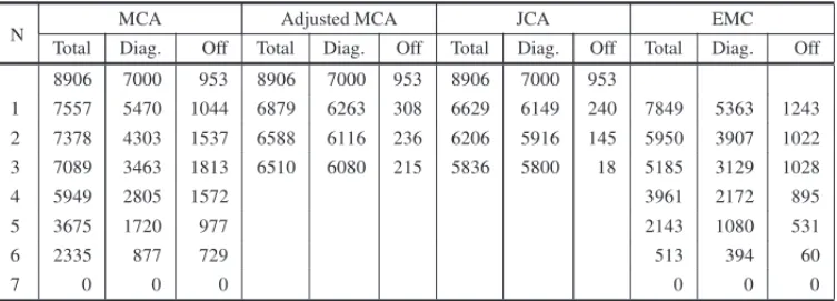
Table 6–Absolute residuals of the reduced dimensional reconstructions of both the Burt’s table
and the two-way off-diagonal ones according toMCA, adjustedMCAandJCArespectively: to 0 correspond the deviations from independence.
MCA Adjusted MCA JCA EMC
N
Total Diag. Off Total Diag. Off Total Diag. Off Total Diag. Off 8906 7000 953 8906 7000 953 8906 7000 953
1 7557 5470 1044 6879 6263 308 6629 6149 240 7849 5363 1243 2 7378 4303 1537 6588 6116 236 6206 5916 145 5950 3907 1022
3 7089 3463 1813 6510 6080 215 5836 5800 18 5185 3129 1028
4 5949 2805 1572 3961 2172 895
5 3675 1720 977 2143 1080 531
6 2335 877 729 513 394 60
7 0 0 0 0 0 0
In Table 6 are reported the cumulate absolute residuals of reconstructions ofMCAs, both normal and adjusted,JCA, andEMC: they are both total and partitioned according to the diagonal ma-trices and the off-diagonal ones. In this latter case, the residuals are divided by two, that is the sum of the residuals of the individual 2×2 contingency tables, that form either triangular off-diagonal sub-matrix. The residuals for 0-dimension are the deviations from independence and the following are reported for all the allowed dimensions: 7= J−Qfor bothMCAandEMC and 3 for both adjustedMCAandJCA, that corresponds to the number of singular values of the Burt’s table larger than the average.
The first row reports the deviations in respect to the independence, that forEMCdoes not make any sense. For each method, the first column represents the inertia of the whole Burt’s table reconstruction: it is always descendant, as it should be expected, although with different slope: in this respect, EMCperforms best by far. Indeed, the same occurs for what concerns the re-construction of the diagonal tables: once again theEMC’s performance is the best, albeit not as for the total table. BothMCAandEMCeventually rebuild totally the Burt’s table, as expected. The surprises arise looking at the off-diagonal tables reconstruction: here, theMCA reconstruc-tion is dramatically bad and problematic: indeed, all partial reconstrucreconstruc-tions are worst than the independence, that is the estimated frequencies are further from the observed than those due the independence, but the last one. That is, the first 5 dimensions, instead of improving the estima-tion, get it even worse! In this respect,EMCperforms much better, as it is constantly decreasing.
4 CONCLUSION
This study started with the aim to understand to what extent theJCA[20] could be of help in identifying the true dimension of an analysis concerning a set of qualitative data. In this sense, the confidence interval proposed by Ben Ammou & Saporta [5, 6] seems a better answer to this problem, that in the proposed example resulted in agreement with the most one-dimensional solution of theSCAs applied to the two-way tables.
During the study, the problem of the data reconstruction not only showed that MCAis bad in reconstructing the whole data table, in respect toEMC, even in what concerns the diago-nal submatrices, but mostly concerning the off-diagodiago-nal ones, that are even more biased: the reconstruction of the two-way off-diagonal tables is for the most reduced-dimensional solu-tions worst than the independence table. Indeed, only redefining the inertia according to the adjustedMCA, a suitable reconstruction may be performed, albeit far from optimality, that is much better approached byJCA. It is interesting to note that, concerning the off-diagonal tables the adjustedMCAseems to perform better than EMC, a result that should be further studied. Eventually, the performance ofJCA, as expected, is by no means the most suitable to deal with the off-diagonal tables, that is on the study of the relations between pairs of characters. As for the interpretation of the factors, JCA is not very different fromMCA, whereas the method’s differences of EMCimpose a different interpretation that may be further studied. Thus, JCA seems the most promising development ofMCAand its properties deserve some further deep-ening, including the three available programs [21, 41, 43]: indeed, a direct comparison of these results with those obtained through Greenacre’s [22] inertia evaluation through regression, may provide further insights on both methods, albeit our critics on the use of chi-square metrics for the whole Burt’s table remain.
Indeed, no direct comparison of the results is strictly correct, since the methods considered in this work use different metrics, either chi-square orEMC, and/or optimize different criteria, as described. In addition,JCA solutions are not nested. These aspects deserve being taken into account while interpreting the results obtained by the different methods. Eventually, address the study in a different framework such as maximum-likelihood estimation, may be a fruitful alternative.
ACKNOWLEDGEMENTS
REFERENCES
[1] ABDI H. 2007. Singular Value Decomposition (SV D) and Generalized Singular Value Decomposition (G SV D). In: SALKINDN (Ed.),Encyclopedia of Measurement and Statis-tics. Thousand Oaks, CA: Sage: pp. 940–945.
[2] ABDIH & VALENTIND. 2007. Multiple Correspondence Analysis. In: SALKINDN (Ed.), Encyclopedia of Measurement and Statistics. Thousand Oaks, CA: Sage: pp. 651–657.
[3] BARTON DE & DAVIDFN. 1956. Some Notes on Ordered Random Intervals.Journal of the Royal Statistical Society, Series B,18(1): 79–94.
[4] BELTON V & STEWART T. 2002.Multiple Criteria Decision Analysis. Boston, Kluwer Academic Publishers.
[5] BENAMMOUS & SAPORTA G. 1998. Sur la normalit´e asymptotique des valeurs propres en ACM sous l’hypoth`ese d’ind´ependance des variables.Revue de Statistique Appliqu´ee, 46(3): 21–35.
[6] BENAMMOUS & SAPORTAG. 2003. On the connection between the distribution of eigen-values in multiple correspondence analysis and log-linear models. REVSTAT-Statistical Journal,1(0): 42–79.
[7] BENZECRI´ JPET AL. 1973-82.L’Analyse des donn´ees, Tome 2. Paris: Dunod.
[8] BENZECRI´ JP. 1979. Sur les calcul des taux d’inertie dans l’analyse d’un questionnaire. Les Cahiers de l’Analyse des Donn´ees,4(3): 377–379.
[9] CAMIZ S. 2005. The Guttman Effect: its Interpretation and a New Redressing Method.
Τετραδ´ια Αναλυσης Δεδομ´ ενων´ (Data Analysis Bulletin),5: 7–34.
[10] CAMIZ S & GOMES GC. 2013. Joint Correspondence Analysis Versus Multiple Corre-spondence Analysis: A Solution to an Undetected Problem. In: GIUSTI A et al. (eds.), Classification and Data Mining, Studies in Classification, Data Analysis, and Knowledge Organization, Berlin, Springer: pp. 11–18.
[11] CAMIZS & PILLARVD. (In press). Identifying the True Dimension in Principal Compo-nent Analysis. Submitted toCommunity Ecology.
[12] CATTELL RB. 1966. The scree test for the number of factors. Multivariate Behavioural Research,1: 245–276.
[13] ECKARTC & YOUNGG. 1936. The approximation of one matrix by another of lower rank. Psychometrika,1: 211–218.
[14] FRAWLEYWJ, PIATETSKY-SHAPIROG & MATHEUSCJ. 1992. Knowledge Discovery in Databases: An Overview,Artificial Intelligence Magazine,13(3): 57–70.
[16] G ´OESART, STEINERMTA & PENICHERA. 2015. Classification of Power Quality Con-sidering Voltage Sags in Distribution Systems Using KDD Process.Pesquisa Operacional, 35(2): 329–352.
[17] GOMESLFAM &DEANDRADERM. 2012. Performance evaluation in assets management with the AHP.Pesquisa Operacional,32(1): 31–53.
[18] GOWERJC & HANDDJ. 1006.Biplots. London, Chapman and Hall.
[19] GREENACRE MJ. 1983.Theory and Application of Correspondence Analysis. London: Academic Press.
[20] GREENACRE MJ. 1988. Correspondence analysis of mutlivariate categorical data by weighted least squares.Biometrika,75: 457–467.
[21] GREENACRE MJ. 2006. From Simple to Multiple Correspondence Analysis. In: GREEN -ACRE& BLASIUS(Eds.), pp. 41–76.
[22] GREENACREMJ. 2007.Correspondence Analysis in Practice, 2nd Ed., London, Chapman and Hall.
[23] GREENACRE MJ & BLASIUSJ. (Eds.) 2006.Multiple Correspondence Analysis and Re-lated Methods. Dordrecht (The Netherlands): Chapman and Hall (Kluwer).
[24] GUTTMANL. 1941. The Quantification of a Class of Attributes: a Theory and Method of Scale Construction. In: HORSTP (Ed.)The Prediction of Personal Adjustment. New York, Social Science Research Council.
[25] JACKSON DA. 1993. Stopping rules in principal component analysis: a comparison of heuristical and statistical approaches.Ecology,74: 2204–2214.
[26] JOLLIFFEIT. 2002. Principal Components Analysis. Berlin, Springer.
[27] LANCASTERHO. 1949. The derivation and partition ofχ2in certain discrete distributions. Biometrika,36: 117–129.
[28] LANCASTERHO. 1963. Canonical Correlations and Partitions ofχ2.Quarterly Journal of Mathematics,14(1): 220–224.
[29] LEBART L. 1976. The significance of Eigenvalues issued from Correspondence Analysis. COMPSTAT, Vienna, Physica Verlag: pp. 38–45.
[30] LOPESYG &DEALMEIDAAT. 2013. A multicriteria decision model for selecting a port-folio of oil and gas exploration projects.Pesquisa Operacional,33(3): 417–441.
[31] MALINVAUD E. 1987. Data analysis in applied socio-economic statistics with special consideration of correspondence analysis. Marketing Science Conference, Joy en Josas: HEC-ISA.
[33] NENADICO & GREENACREM. 2006.Computation of multiple correspondence analysis, with code in R. In: GREENACRE ANDBLASIUS(Eds), (2006), pp. 523–551.
[34] NENADICO & GREENACREM. 2007. Correspondence analysis in R, with two- and three-dimensional graphics: thecapackage.Journal of Statistical Software,20(3): 1–13. [35] ORLOCI´ L. 1978.Multivariate Analysis in Vegetation Research, 2nd ed.. Den Haag: Junk.
[36] PERES-NETO PR, JACKSON DA & SOMERS KM. 2005. How Many Principal Compo-nents? Stopping Rules for Determining the Number of Non-trivial Axes Revisited. Compu-tational Statistics and Data Analysis,49: 974–997.
[37] ROYB & BOUYSSOU D. 1985.Aide `a la d´ecision: m´ethodes et cas. Paris, Economica.
[38] R-PROJECT. 2009. http://www.r-project.org/
[39] SAPORTA G. 1975.Liaison entre plusieurs ensembles de variables et codage de donn´ees qualitatives. Th`ese de troisi`eme cycle, Paris VI, Universit´e Pierre et Marie Curie.
[40] SASSI RJ. 2012. An Hybrid Architecture for Clusters Analysis: Rough Sets Theory and Self-Organizing Map Artificial Neural Network.Pesquisa Operacional,32(1): 139–163. [41] TATENENI K & BROWNEMW. 2000. A Noniterative Method of Joint Correspondence
Analysis.Psychometrika,65(2): 157–165.
[42] THOMSONGH. 1934. Hotelling’s method modified to give Spearman’s g.Journal of Edu-cational Psychology,25: 366–374.
[43] VERMUNTJK & ANDERSONC. 2005. Joint Correspondence Analysis (JCA) by Maximum Likelihood,European Journal of Research Methods for the Behavioral and Social Sciences, 1(1): 18–26.