doi: 10.1590/0101-7438.2015.035.01.0123
ON HYPOTHESIS TESTS FOR COVARIANCE MATRICES UNDER MULTIVARIATE NORMALITY
Let´ıcia Pereira Pinto
1and Sueli Aparecida Mingoti
2*Received June 11, 2012 / Accepted April 06, 2014
ABSTRACT.In this paper we proposed a new statistical test for testing the covariance matrix in one population under multivariate normal assumption. In general, the proposed and the likelihood-ratio tests resulted in larger values of estimated powers than VMAX for bivariate and trivariate cases. VMAX was not sensitive to general changes in the covariance (correlation) structure. The advantage of the new test is that it is based on the comparison of all elements of the postulated covariance matrix under the null hypothesis with their respective maximum likelihood sample estimates and therefore, it does not restrict the information of the covariance matrix into a scalar number such as the determinant or trace, for example. Due to the fact that it is based on the maximum likelihood estimates and the Fisher information matrix, it can be used for data coming from distribution other than the multivariate normal.
Keywords: covariance matrix, hypothesis testing, Fisher information matrix.
1 INTRODUCTION
Statistical tests for covariance matrix has been the issue of many papers particularly in qual-ity control for monitoring processes using several qualqual-ity characteristics simultaneously, or in calibrations studies (Li & Tsung, 2011). They are also used to verify the assumption of equal co-variance matrices when performing statistical tests to compare the vector means of independent populations, such as in marketing research in the comparison of consumers profiles of different segments, among many other applications (Montgomery, 2008).
A well-known statistical test used to verify if the covariance matrix of a population (or process) has a certain specified structure is the generalized variance,|S|, which is based on the determinant of the sample covariance matrix (see Alt, 1985; Djauhari, 2005). Tests based on transformations of|S|are also found in the literature (Garc´ıa-Diaz, 2007). Although the idea of summarizing the information of the covariance matrix into a scalar number is appealing, the fact that different
*Corresponding author.
matrices can have equal or similar determinants makes the generalized variance to fail in detect-ing some types of changes in the covariance matrix when they take place. The assumption of a normal distribution as an approximated distribution for|S|, may also restrict its use in certain areas since it just holds for large sample sizes (Djauhari, 2009). In quality control, for example, it is common to use samples of sizes n = 4 or 5, cases for which the normal approximation would not be valid. The exact distribution of|S|for the bivariate case is known and it is related to a chi-square distribution. However, for p >2 variables the exact distribution of|S|does not belong to any class of known probability distributions (Anderson, 1958; Aparisi et al., 1999).
The likelihood-ratio test was presented by Anderson (1958), in a general context for multivariate normal populations and by Alt (1985), as a tool to monitor the covariance matrix in quality control. However, the test was based on the chi-square distribution for the test statistic which is valid asymptotically, only. Costa & Machado (2009; 2008), proposed the VMAX based on the maximum of the p standardized sample variances, p being the number of variables or quality characteristics. VMAX was more efficient than the generalized variance to monitor processes presenting better capability at detecting variances shifts. The critical region of the test (or control chart) was obtained by numerical integration which involves non-central chi-square distributions. More recently, Quinino et al. (2012), proposed the VMIX as a tool to monitor the variability structure of two quality characteristics under the assumption of bivariate normal distribution. In their paper it was shown that VMIX was more efficient than the generalized variance control chart and better than VMAX, for some cases.
A more general method was proposed by Sullivan et al. (2007), considering the vector of parameters θ which includes the elements of the mean vector and the covariance matrix. The estimated vector ofθ is compared with the vectorθ specified in the null hypothesis by means of a test statistic which has an approximated chi-square distribution under the null hypothesis. What is interesting in Sullivan et al. (2007) test is that there is no restriction on the structure of the covariance matrix postulated on the alternative hypothesis and it can be used for normal and non-normal distributions being capable of testing the whole vector of parameters as well as parts of it. As an illustration for the bivariate case, one could be interested in testing the vectorθ containing all 5 parameters (two means, two variances and one covariance); the parameter vector θ containing the two means or two variances only, or containing just the variances and the co-variances, among other possibilities. Other statistical tests for covariance matrices can be found in the literature (see Yeh et al., 2006; 2012, among others).
2 STATISTICAL TESTS FOR COVARIANCE MATRICES
For all tests presented it this section, it is assumed that X1,X2, . . . ,Xn, where Xk = (Xk1,Xk2, . . . ,Xkp)′,k = 1,2, . . . ,n, is a random sample of sizen from a p-variate normal distribution with the mean vector µ = (µ1, µ2, . . . , µp)′ and covariance matrix, a p× p
positive definite matrix, where pis the number of random variables.
2.1 The likelihood-ratio test
The likelihood-ratio is a well-known method of hypothesis testing (Alt, 1985; Casella & Berger, 2002), and it can be used to construct a test for the covariance matrix as follows. Under the
p-variate normal distribution assumption, the likelihood function is given as
L(x1,x2, . . . ,xn)=
1 (2π )np/2||n/2
n
k=1
exp
−1
2(xk−µ) ′−1(x
k−µ)
(1)
where xk = (xk1,xk2, . . . ,xkp)′ is the observed vector for the kth sample element, k = 1,2, . . . ,n, and |.|denotes the determinant of the matrix. Let the null and the alternative hy-pothesis be defined as H0: =0, H1: =0,µunknown. Under the null hypothesis the
maximum (Lo) of the likelihood function (1) is achieved when the vector µ is taken as the sample mean vector x¯ and=0. Under the whole parametric space the maximum (L1) is
achieved when the vectorµis taken as the sample mean vectorx¯ and the covariance matrix is estimated as, whereˆ
¯ x= 1
n n
k=1
xk; ˆp×p=
(n−1)
n Sp×p (2)
Sp×p=(n−1)−1n
k=1(xk− ¯x)(xk− ¯x)′is the sample covariance matrix. The likelihood-ratio test statistic is then given by
W = −2 ln(L0/L1)= −pn+pnln(n)−nln
A
−1 0
+tr
0−1A (3)
where A = (n −1)S andtr(.) is the trace operator. The distribution ofW under the null hy-pothesis is asymptotically chi-square andH0is rejected for values ofW larger than the constant
L SC =χα,2p(p+1)/2, which is a value taken from a chi-square distribution withp(p+1)/2 de-grees of freedom, whose area above is equal to the significance level of the test,α,0< α <1. In the quality control terminologyαis the false alarms rate. When the vector meanµis known under the null hypothesis, the test statistic in (3) reduces to
W = −2 ln(L0/L1)= −pn−nln0−1ˆ
+ntr
−01ˆ
(4)
whereˆ =(n)−1n
k=1(xk −µ)(xk−µ)′.
2.2 The VMAX test
(X1,X2)′ be the random vector of interest andH0: =0, H1: =1, be the null and the
alternative hypothesis, where
0=
σ12 σ12 σ21 σ22
and 1=
a2σ12 abσ12
abσ21 b2σ22
a >0,b >0 are constants,σ12,σ22andσ12 =σ21 are the variances and the covariances ofX1
andX2, respectively, under the null hypothesis;a2σ12,b2σ22andabσ12, are the variances and the
covariances of X1and X2, respectively, under the alternative hypothesis. Under this structure,
changes in the variances and covariances values of X1 andX2 are allowed but the correlation
structure is not affected by the changes.
The VMAX test statistic is defined as
V M AX =max{S12,S22} (5)
where
S12=
n
k=1(xk1−µ1)2
nσ12 ; S
2 2=
n
k=1(xk2−µ2)2
nσ22 ,
(xk1,xk2),k =1,2, . . . ,n, are the sample values of the random vectorX = (X1,X2)′. For a
given significance levelα, 0 < α < 1, the critical region of the test is obtained by solving the equation (6) forCL, consideringa=b=1. The null hypothesis is then rejected for any value of (5) larger than the critical constantCL. In the quality control field the constantCLis the control limit.
α=1−
nC L/a2
0
Pr
χ2
n,(tρ2/1−ρ2)<
nC L b2(1−ρ2)
e−t/2
2n/2Ŵn 2
t
(n/2)−1dt (6)
where χ2
n,(tρ2/1−ρ2) represents a chi-square distribution with n degrees of freedom and non-centrality parameter given bytρ2/(1−ρ2), Ŵ(.) is the Gamma function,ρ is the correlation coefficient betweenX1andX2and Pr[.]denotes the probability of the considered event. Under
the alternative hypothesis the expression in (5) is used to compute the power of VMAX test. When the means(µ1, µ2)are unknown, they can be replaced by the respective sample means.
Details about the equation (6) can be found in the Appendix of Costa & Machado’s (2008; 2009) papers. Basically, it was derived taking into consideration the fact that under the bivariate normal distribution assumption,n S12a2has a chi-square distribution withndegrees of freedom (χn2). It can also be shown that conditioned onxk=(xk1,xk2, . . . ,xkp)′, the random variable defined as
n S22
b2(1−ρ2)
has a non-central chi-square distribution withndegrees of freedom and non-centrality parameter given as(ρ21−ρ2)χn2. The equation (6) follows taking into account that
pw =1−Pr(S12≤C L)∩(S22≤C L)
where pw = αwhena =b = 1 (under the null hypothesis), and pw is the power of the test
Costa & Machado (2008), also considered the case where the covariance matrix1was defined
as
1=
a2σ12 σ12 σ21 b2σ22
.
In this case, under the alternative hypothesis the correlation coefficient betweenX1andX2would
change toρ=σi j/abσ1σ2, whereσ1, σ2, are the standard deviations of the variablesX1andX2,
respectively.
VMAX test was extended by Costa & Machado (2009), for the multivariate case (p > 2) by using a similar approach as taken to the bivariate normal population. Numerical integration was used to obtain the critical constantCLof the test.
2.3 Sullivan et al. (2007) statistical test
Sullivan et al. (2007), proposed a statistical test that can be applied for two groups of consecutive independent homogeneous observations with the purpose of comparing the parameters of the distributions of both groups. This test is of importance in quality control since it can be used to compare the process parameters before and after some identified change point in the structure of the sample observations. In a more general context Sullivan et al. (2007) test could be applied in the comparison of the vector means and/or the covariance matrices of two independent groups.
Let’s suppose that the parameters of the distributions before (A) and after (B) the change point, are described by the parameter vectorθ which consists of the elements of the vector meanµ and the covariance matrix. As an illustration, for the bivariate normal distribution the vector θcan be defined asθ =(µ1, µ2, σ12, σ12, σ22)′orθ =(µ1, µ2, σ1, ρ12, σ2)′, whereσ12andρ12
are the covariance and correlation between the two variables andσi is the standard deviation of the variableXi,i =1,2. LetθAandθB be the parameter vectors of the groups of observations AandB respectively, andθˆA andθˆB be their respective maximum likelihood estimators. Let the (k0 ×1) vector δˆ = (θˆA− ˆθB), be the maximum likelihood estimator of the difference vectorδ=(θA−θB), wherek0is the number of parameters being compared. As well known,
under general regularity conditions, the maximum likelihood estimators have asymptotically a multivariate normal distribution (Casella & Berger, 2002). Therefore, under the null hypothesis, asymptotically, the quadratic form
χA2,B = ˆδ′ˆ−δˆ1δˆ
has a chi-square distribution withk0 degrees of freedom, whereδ andδˆ are the theoretical and the estimated covariance matrices ofδ, respectively. The null hypothesis corresponds to theˆ non-changing in the vector of parameters, i.e.,δ=0. The covariance matrixδˆis approximated by the Fisher information matrix (Casella & Berger, 2002), and it is estimated by using an al-gebraic expression for the expected value of the Hessian matrix, which is then evaluated at the maximum likelihood estimates of the parameters.
2.4 An Adaptation of Sullivan et al. (2007) to test the covariance matrix
In this section we will describe an adaptation of the Sullivan et al. (2007) test for the situation in which only the covariance matrix of the population is concerned. From all over this paper we will call this test as an adapted Sullivan et al.
Let p = 2, µ1 andµ2 pre-specified and θ = (σ1, ρ12, σ2)′ be the parameter vector from a
bivariate normal distribution. Letθˆbe the vector containing the maximum likelihood estimates of the parameters inθ. LetH0:θ=θ0andH1:θ =θ1, be the null and the alternative hypothesis
which are equivalent to H0: δ=0 and H0: δ=0, whereδ=θ−θ0. Let the test statistic be
defined as
χs2=δˆ′−ˆ1 δ
ˆ
δ (7)
whereδˆ= ˆθ−θ0. UnderH0, asymptotically, the test statistic in (7) has a chi-square distribution
withk0=3 degrees of freedom being the null hypothesis rejected for large values of (7),
accord-ing to the significance level of the test. Under the bivariate normality assumption the covariance matrixδˆis obtained through the Fisher information matrix (see Beyer, 1978; Sullivan et al., 2007), which is given by
δˆ=
⎡
⎢ ⎣
d −e f
−e h −g
f −g i
⎤
⎥
⎦ (8)
where
d =σ
2 1
2n, e=
ρ12(ρ122 −1)σ1
2n , f =
ρ122σ1σ2
2n ,
g=ρ12(ρ
2 12−1)σ2
2n , h=
(ρ212−1)
n and i =
σ22
2n,
being the values ofσ1,σ2,ρ12,σ12,σ22,σ12 as specified inH0, whereσ12, σ22are the variances
ofX1andX2variables, respectively.
The adapted Sullivan et al. test for the covariance matrix can also be extended for p > 2 variables. Let X be a(p×1)random vector with multivariate normal distribution, with mean vector µ(θ )and covariance matrix (θ ), where µ(θ ) = (µ1(θ ), µ2(θ ), . . . , µp(θ ))′. In this case the typical (i,j) element of the Fisher information matrix is given by
Ii,j = ∂µ ∂θi
−1∂µ′ ∂θj
+1 2tr
−1∂ ∂θi
−1∂ ∂θj where ∂µ ∂θi = ∂µ1 ∂θi , ∂µ2 ∂θi , ...,
∂µp ∂θi ; ∂ ∂θi = ⎡ ⎢ ⎢ ⎢ ⎢ ⎢ ⎢ ⎢ ⎢ ⎢ ⎢ ⎣
∂1,1 ∂θi
∂1,2 ∂θi . . .
∂1,p ∂θi
∂2,1
∂θi
∂2,2
∂θi . . .
∂2,p
∂θi ..
. ... ... ...
∂p,1 ∂θi
∂p,2 ∂θi
· · · ∂p,p
tr(.)is the trace operator andi,j is the (i,j) element of the covariance matrix.
A possible advantage of the adapted Sullivan et al. test regarding to the VMAX and the like-lihood-ratio tests comes from the fact that all the parameters of the covariance matrix postulated in the null hypothesis are compared in its test statistic, one by one, with their respective max-imum likelihood estimates, so that there is no reduction of the covariance matrix information into a single measure such as the determinant, or others. It also allows the correlation coeffi-cients under the null and the alternative hypothesis to be completely different being therefore, a more general test. The test can also be used for non-normal multivariate data since it is based on the maximum likelihood estimates and the Fisher information matrix. It also can be used to test shifts in the variances of the variables only.
3 COMPARISON OF THE STATISTICAL TESTS
The power of the adapted Sullivan et al., the VMAX and the likelihood-ratio tests were esti-mated by using Monte Carlo simulation under the multivariate normal distribution assumption. The null hypothesis isH0: =0, where0is pre-specified. For the adapted Sullivan et al. test as well as for the likelihood-ratio, the exact and the asymptotic chi-square distributions of the test statistics were also consider to determine the respective rejection regions ofH0.
In this paper, in the implementation of the VMAX test for the bivariate normal distribution, the Gauss-Legendre and the Pegasus method were used to sort out the numeric integration and to determine the zeros of the function given in (6) in Section 2.2 (see Davis & Rabinowitz, 1984, for details). Due to the fact that the values ofCLforp=2 obtained by using numeric integration were similar to those obtained by using simulation, the value ofCLfor p =3 was obtained by simulation only.
In order to determine the critical region of the tests by the exact distribution (except for VMAX, p=2), M =50.000 random samples of fixed sizesn =5, 10, 25, 50 and 100 were generated from ap-variate normal distribution with mean vectorµand covariance matrix0as stipulated in the null hypothesis. For each sample the respective test statistic was calculated and the empir-ical distribution was built based on theMobtained sample values. By using this distribution the critical region of the test was determined according to the pre-specified significance levelα= 0.05 for the tests. After the determination of the critical region, the respective type I error and power of the tests were estimated as follows. First, 10.000 random samples were generated from a multivariate normal distribution under the null hypothesis considering=0. For each sam-ple and each test, the null hypothesis was tested and the proportion of rejection was calculated given an estimate of type I error of the test. Afterwards, 10.000 samples were generated from a multivariate normal distribution under the alternative hypothesis, H1: =1, considering
all 50 repetitions for each test, respectively. Without loss of generality this study was performed considering one particular structure for the matrix0forp =2,3 and assumingµ=0under H0andH1.
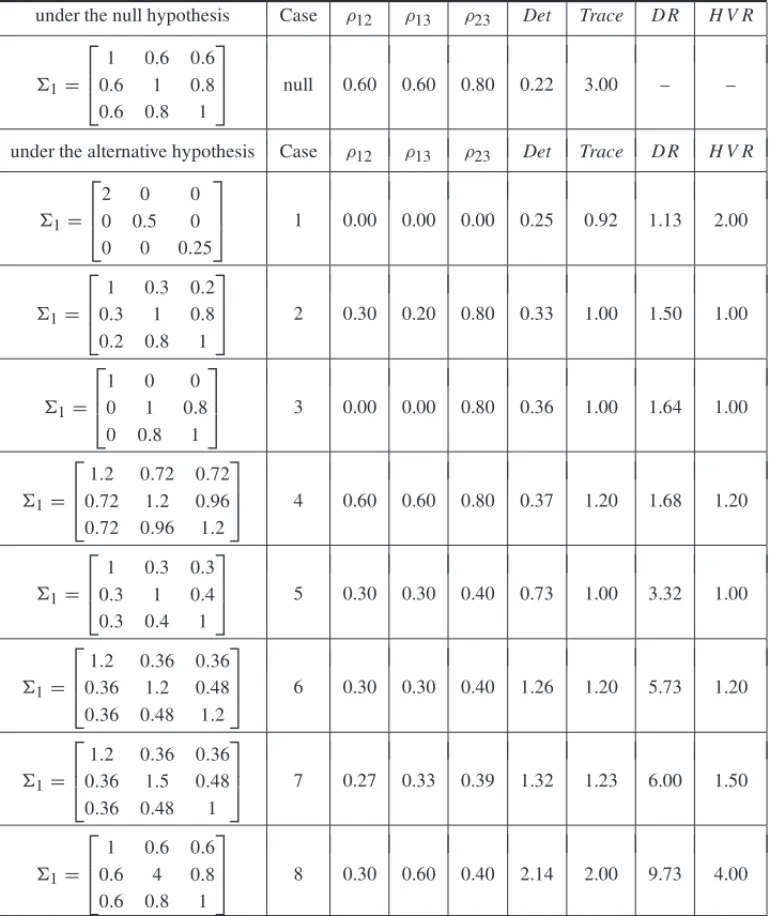
The simulated models under the alternative hypothesis (see Tables 1 and 2), were chosen to make it possible to evaluate whether the traditional likelihood-ratio, the adapted Sullivan et al. and the VMAX tests were able to detect small and large differences from0. In models 1-6 forp =2, and models 1, 6, 7 for p = 3, changes in the variances and in the correlation structure were allowed. Models 7-10 for p=2, 4 and 8 forp=3, were more restrict since the variances were allowed to change but the correlation (in model 4) and the covariance (in model 10) structures remained the same as under the null hypothesis. On the contrary, the models 2, 3 and 5 forp=3, have the same variances asH0but different correlation and covariance structures.
Tables 1 and 2 also present the ratio of the covariance matrices traces and determinants under H0andH1as well as the ratio of the maximum of the variances under the alternative and null
simulated models. The ratio of the determinants for the bivariate models ranged from 1 (cases 2 and 3) to 2.67 (case 5), which corresponds to an increase of 0 to 166,67% in the determinant underH1compared to the determinant underH0. For the trivariate models the ratio ranged from
1.13 to 9.73 (case 8).
3.1 Comparison by using the exact distribution of the tests statistics
The average proportions of rejection of H0for each test discussed in this paper are shown in
Tables 3 and 4, for p=2, under the null and the alternative hypothesis models. When the exact distribution was used to build the critical region of the tests, the estimates of the type I error were 0.05 as expected. Considering only the exact distributions of the test statistics, the adapted Sullivan et al. test (SE) performed better than the likelihood-ratio (LRE) for all sample sizes except in cases 2, 4 and 5, forn =50 and 100, cases which both tests were similar. Compared to VMAX the SE test presented larger power values in cases 1-6 for all sample sizes. Both tests had similar performance for cases 7-10 with some advantage to VMAX for smaller sample sizes.
Table 1– Simulated models−p=2 variables.
under the null hypothesis Case ρ12 σ1 σ2 Trace Det H V R
0=
1 0.5 0.5 1
null 0.50 1.00 1.00 2.00 0.75 –
under the alternative hypothesis Case ρ12 σ1 σ2 T R D R H V R
0=
1 0 0 1
1 0.00 1.00 1.00 1.00 1.33 1.00
0=
1 −0.50
−0.50 1
2 –0.50 1.00 1.00 1.00 1.00 1.00
0=
1 0 0 1.13
3 0.00 1.00 1.06 1.07 1.51 1.13
0=
1 0 0 1.25
4 0.00 1.00 1.12 1.13 1.67 1.25
0=
1 0 0 2
5 0.00 1.00 1.41 1.50 2.67 2.00
0=
2.32 0 0 0.63
6 0.00 1.52 0.79 1.48 1.95 2.32
0=
1 0.53 0.53 1.13
7 0.50 1.00 1.06 1.07 1.13 1.13
0=
1 0.56 0.56 1.25
8 0.50 1.00 1.12 1.13 1.25 1.25
0=
1 0.71 0.71 2
9 0.50 1.00 1.41 1.50 1.99 2.00
0=
2.32 0.61 0.61 0.63
10 0.50 2.32 1.52 1.48 1.45 2.32
(*)Det: determinant;T RandD R: ratios between the traces and the determinants of the covariance
matrices underH1andH0, respectively;H V R: ratio between the maximum of the variances underH1
andH0.ρ12is the correlation between both variables.σiis the standard deviation of variableX1,i=1,2.
of sizen=5 (power=0.29) reaching a power equal 0.74 forn =25 (for this particular value of n, the power values of SE and LRE were 0.96 and 0.93, respectively). That is not very surprising since the test statistic of VMAX is based only upon the maximum ratio between the sample and the population variances postulated in the null hypothesis.
Table 2– Simulated models−p=3 variables.
under the null hypothesis Case ρ12 ρ13 ρ23 Det Trace D R H V R
1= ⎡
⎢ ⎣
1 0.6 0.6 0.6 1 0.8 0.6 0.8 1
⎤
⎥
⎦ null 0.60 0.60 0.80 0.22 3.00 – –
under the alternative hypothesis Case ρ12 ρ13 ρ23 Det Trace D R H V R
1= ⎡
⎢ ⎣
2 0 0
0 0.5 0 0 0 0.25
⎤
⎥
⎦ 1 0.00 0.00 0.00 0.25 0.92 1.13 2.00
1= ⎡
⎢ ⎣
1 0.3 0.2 0.3 1 0.8 0.2 0.8 1
⎤
⎥
⎦ 2 0.30 0.20 0.80 0.33 1.00 1.50 1.00
1= ⎡
⎢ ⎣
1 0 0
0 1 0.8 0 0.8 1
⎤
⎥
⎦ 3 0.00 0.00 0.80 0.36 1.00 1.64 1.00
1= ⎡
⎢ ⎣
1.2 0.72 0.72 0.72 1.2 0.96 0.72 0.96 1.2
⎤
⎥
⎦ 4 0.60 0.60 0.80 0.37 1.20 1.68 1.20
1= ⎡
⎢ ⎣
1 0.3 0.3 0.3 1 0.4 0.3 0.4 1
⎤
⎥
⎦ 5 0.30 0.30 0.40 0.73 1.00 3.32 1.00
1= ⎡
⎢ ⎣
1.2 0.36 0.36 0.36 1.2 0.48 0.36 0.48 1.2
⎤
⎥
⎦ 6 0.30 0.30 0.40 1.26 1.20 5.73 1.20
1= ⎡
⎢ ⎣
1.2 0.36 0.36 0.36 1.5 0.48 0.36 0.48 1
⎤
⎥
⎦ 7 0.27 0.33 0.39 1.32 1.23 6.00 1.50
1= ⎡
⎢ ⎣
1 0.6 0.6 0.6 4 0.8 0.6 0.8 1
⎤
⎥
⎦ 8 0.30 0.60 0.40 2.14 2.00 9.73 4.00
(*)Det: determinant;T RandD R: ratios between the traces and the determinants of the covariance matrices
underH1andH0, respectively;H V R: ratio between the maximum of the variances underH1andH0.ρi j is the correlation between variables.XiandXj,i=j.
Table 3– Type I error and power estimates of the tests−p=2,n=5, 10 and 25. Average proportion of rejection of the null hypothesis
n=5 n=10 n=25
Case LRE SE VMAX LRE SE VMAX LR LRE SC SE VMAX
null 0.05 0.05 0.05 0.05 0.05 0.05 0.07 0.05 0.06 0.05 0.05 1 0.10 0.25 0.05 0.23 0.43 0.05 0.67 0.63 0.79 0.77 0.05 2 0.29 0.58 0.05 0.72 0.89 0.05 1.00 1.00 1.00 1.00 0.05 3 0.11 0.27 0.07 0.26 0.46 0.08 0.71 0.67 0.81 0.79 0.10 4 0.11 0.29 0.09 0.28 0.49 0.12 0.75 0.72 0.84 0.82 0.17 5 0.20 0.41 0.29 0.50 0.68 0.44 0.94 0.93 0.96 0.96 0.74 6 0.26 0.45 0.36 0.62 0.75 0.55 0.98 0.98 0.99 0.98 0.87 7 0.05 0.06 0.08 0.05 0.07 0.08 0.08 0.06 0.09 0.07 0.10 8 0.05 0.07 0.10 0.06 0.08 0.12 0.11 0.09 0.14 0.12 0.17 9 0.09 0.18 0.29 0.21 0.33 0.46 0.61 0.57 0.68 0.65 0.74 10 0.16 0.26 0.37 0.43 0.52 0.56 0.91 0.89 0.92 0.92 0.87
(*) LR and LRE: are the likelihood-ratio using chi-square approximation and the exact distributions; SC and
SE are the adapted Sullivan et al. using chi-square approximation and the exact distributions; VMAX test
using the exact distribution.
Table 4– Type I error and power estimates of the tests−p=2,n=50 and 100. Average proportion of rejection of the null hypothesis
n=50 n=100
Case LR LRE SC SE VMAX LR LRE SC SE VMAX
null 0.06 0.05 0.06 0.05 0.05 0.05 0.05 0.05 0.05 0.05 1 0.93 0.93 0.96 0.96 0.05 1.00 0.93 1.00 1.00 0.05 2 1.00 1.00 1.00 1.00 0.05 1.00 1.00 1.00 1.00 0.05 3 0.95 0.95 0.97 0.97 0.13 1.00 0.95 1.00 1.00 0.18 4 0.96 0.96 0.98 0.98 0.25 1.00 0.96 1.00 1.00 0.41 5 1.00 1.00 1.00 1.00 0.94 1.00 1.00 1.00 1.00 1.00 6 1.00 1.00 1.00 1.00 0.99 1.00 1.00 1.00 1.00 1.00 7 0.08 0.07 0.10 0.09 0.13 0.11 0.11 0.13 0.13 0.18 8 0.16 0.14 0.19 0.18 0.26 0.28 0.27 0.31 0.31 0.40 9 0.89 0.88 0.92 0.91 0.94 0.99 0.99 0.99 0.99 0.99 10 0.99 0.99 0.99 0.99 0.99 1.00 1.00 1.00 1.00 1.00
(*) LR and LRE are the likelihood-ratio tests using chi-square and the exact distributions. SC and
SE are the adapted Sullivan et al. test using chi-square and the exact distributions. VMAX is the
values (around 1). On the other hand, the performance of VMAX increased but the SE was still very competitive.
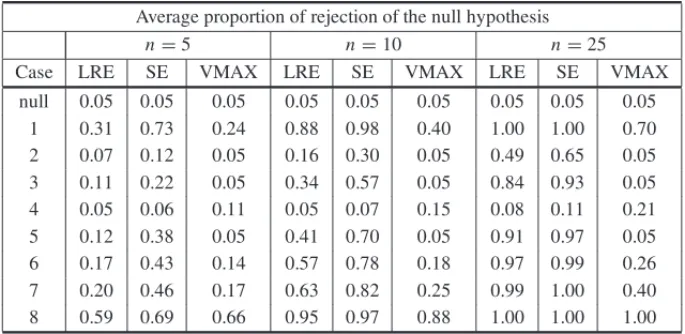
Tables 5 and 6 present the estimates of type I error and power for p=3. Considering only the exact distributions to compare the tests (they all reach 0.05 type I error under the null hypothesis), it can be seen that the VMAX did not perform well for cases 2, 3 and 5 (estimated power 0.05 for all sample sizes). These results are expected since the test statistic of VMAX just takes into account changes in variances of the variables. For these models the adapted Sullivan et al. was more efficient than the maximum likelihood ratio test (SE: power≥0.30; LRE power≥0.16, for n ≥10), particularly for case 5 (power=0.38 forn =5 and≥0.70 forn≥10). That was due to the fact that1and0have equal diagonal values although completely different covariance structures.
Table 5– Type I error and power estimates of the tests−p=3,n=5, 10 and 25. Average proportion of rejection of the null hypothesis
n=5 n=10 n=25
Case LRE SE VMAX LRE SE VMAX LRE SE VMAX null 0.05 0.05 0.05 0.05 0.05 0.05 0.05 0.05 0.05
1 0.31 0.73 0.24 0.88 0.98 0.40 1.00 1.00 0.70 2 0.07 0.12 0.05 0.16 0.30 0.05 0.49 0.65 0.05 3 0.11 0.22 0.05 0.34 0.57 0.05 0.84 0.93 0.05 4 0.05 0.06 0.11 0.05 0.07 0.15 0.08 0.11 0.21 5 0.12 0.38 0.05 0.41 0.70 0.05 0.91 0.97 0.05 6 0.17 0.43 0.14 0.57 0.78 0.18 0.97 0.99 0.26 7 0.20 0.46 0.17 0.63 0.82 0.25 0.99 1.00 0.40 8 0.59 0.69 0.66 0.95 0.97 0.88 1.00 1.00 1.00
(*) LR and LRE are the likelihood-ratio tests using chi-squared and the exact distributions.
SC and SE are the adapted Sullivan et al. test using chi-squared and the exact distributions.
VMAX is the test using the exact distribution.
Table 6– Type I error and power estimates of the tests−p=3,n=50 and 100. Average proportion of rejection of the null hypothesis
n=50 n=100
Case LR LRE SC SE VMAX LR LRE SC SE VMAX
null 0.06 0.05 0.07 0.05 0.05 0.06 0.05 0.05 0.05 0.05 1 1.00 1.00 1.00 1.00 0.93 1.00 1.00 1.00 1.00 1.00 2 0.86 0.84 0.93 0.92 0.05 1.00 1.00 1.00 1.00 0.05 3 0.99 0.99 1.00 1.00 0.05 1.00 1.00 1.00 1.00 0.05 4 0.17 0.14 0.24 0.20 0.30 0.33 0.31 0.40 0.37 0.46 5 1.00 1.00 1.00 1.00 0.06 1.00 1.00 1.00 1.00 0.06 6 1.00 1.00 1.00 1.00 0.37 1.00 1.00 1.00 1.00 0.55 7 1.00 1.00 1.00 1.00 0.61 1.00 1.00 1.00 1.00 0.86 8 1.00 1.00 1.00 1.00 1.00 1.00 1.00 1.00 1.00 1.00
(*) LR and LRE are the likelihood-ratio tests using chi-squared and the exact distributions.
SC and SE are the adapted Sullivan et al. test using chi-squared and the exact distributions.
VMAX is the test using the exact distribution.
equal 1.0 forn ≥ 25. The best values for VMAX occurred forn =50 (power=0.61) and for n=100 (power=0.86).
Althoughn = 5 is a small sample size to test hypothesis about the covariance matrix when p =3, the adapted Sullivan et al. performed well for the cases 1, 6 and 7, (power: 0.73, 0.43 and 0.46, respectively), being the estimated power about 3 times larger than VMAX and 2.5 larger than LRE values.
The efficiency of VMAX in detecting the shifts of the covariance matrix improved a lot for case 8 (power:≥ 0.66;=1.0 forn ≥ 25), case which the covariance structure remains the same as H0but the variance of the second variable (see1) is 4 times larger than the value giving in0.
For this particular case, VMAX power estimates were closer to the SE and LRE values.
Comparing the results of cases 4 and 6 (both haveH V R =1.2, see Table 2), it is possible to see that the different correlation structure affected the SE and LRE efficiencies since the tests were more powerful to detect the shits in case 6 than in the case 4. This result is due to the fact that the values of SE and LRE test statistics take into account all the variances and covariances values from the0and1matrices, and the matrix1of case 4 is more similar to0than the covariance matrix of case 6. Both SE and LRE did not perform well in case 4 and VMAX had power estimates larger than these two tests (maximum power estimates: VMAX=0.46; SE= 0.37; LRE=0.31). It is important to point out that cases 4 and 8 belong to the framework which VMAX was proposed by Costa & Machado (2008; 2009) since only increases of variances were allowed being the correlation, or the covariance, structures the same as inH0. Therefore, the
re-sults suggest that under this framework the performance of VMAX is similar to the performance of the adapted Sullivan et al. test.
Considering all the results observed for p = 2 and 3, we can conclude that for the evaluated cases, when the exact distribution was used to build the critical region of the tests, the adapted Sullivan et al. was more efficient than the maximum likelihood-ratio, both were more efficient than VMAX with few exceptions. The exceptions were related to the cases whose variances changed but the correlation (or the covariance) structure under the alternative hypothesis was kept the same as inH0, situations that fit well in the framework of VMAX test. One of the main
goals in quality control is to detect variances increases and in this context the results showed that VMAX performed well.
3.2 Discussion of the results from the asymptotic distribution of the test statistic
As far as the chi-square approximation is concerned, for the bivariate cases and small samples sizes (n = 5 and 10) the maximum likelihood-ratio (LR) and the adapted Sullivan et al. (SC) tests resulted in estimates of type I error larger than the pre-specified nominal significance level of 5% (estimates were 19 and 10% respectively, for LR; 12 and 8% for SC). Therefore, their power estimates could not be compared with the results from the exact distributions of the tests and were not presented in Table 3. For samples of sizesn =25 and 50 the estimates were more reasonable (around 6 to 7%) and equal 5% forn =100. This is perfectly explained by the fact that the chi-square approximation is valid only for larger sample sizes. Forn ≥ 25 the average power estimates from the chi-square distribution are shown in Tables 3 and 4. The results were similar to the estimates obtained by the exact distributions.
Similar pattern was found for p =3. For small samples (n =5,10), the estimates of the type I error based on the chi-square distribution were also much larger than the pre-specified 5% significance level. For the maximum likelihood ratio test (LR), the estimates were equal 37% forn =5, 14% forn =10, 8% forn =25, being the approximation to 5% achieved only for samples of sizes 50 and 100 (estimates around 5 to 6%). For the adapted Sullivan et al. test (SC), the estimates were 22, 14 and 9% forn = 5, 10 and 25, respectively, achieving 5% only for larger samples (estimates around 7 to 5% forn =50 and 100). Forn ≥50 the average power estimates from the chi-square distribution are shown in Tables 5 and 6 for the LR an SC tests and the results were similar to the estimates obtained by the exact distribution.
Therefore, by the results presented for p = 2,3, it is clear that the chi-square approximation did not work well for small sample sizes being not recommended in these situations. The exact distribution of the test statistics obtained by Monte Carlo simulation should be used for small sample sizes.
4 EXAMPLES OF APPLICATION
Example 1. The transpiration data of 20 healthy females was given on Table 5.1 from Johnson & Wichern (2002). The variables of interest were: rate of sweat (X1), quantity of sodium (X2)
and quantity of potassium (X3). Suppose the researcher wants to test the null hypothesisH0 :
=0againstH1:=0, where
0=
⎡
⎢ ⎣
3 11 2
11 200 6
2 6 3.74
⎤
⎥ ⎦
By the data from Johnson & Wichern (2002), one can find the maximum likelihood estimate of the population covariance matrix as
ˆ
=
⎡
⎢ ⎣
2.735 9.509 −1.718 9.509 189.798 −5.937 −1.718 −5.937 3.447
⎤
⎥ ⎦
The parameter vector under the null hypothesis, the respective maximum likelihood vector esti-mate and the difference between these two vectors are given by
θ0=(σ1, ρ12, σ2, ρ13, ρ23, σ3)′=(1.732, 0.449, 14.142, 0.597, 0.219, 1.933)′
ˆ
θ=(1.654, 0.417, 13.776, −0.559, −0.232, 1.856)′
ˆ
δ = ˆθ−θ0=(−0.078, −0.032, −0.366, −1.156, −0.451, −0.076)′.
The results of the three tests discussed in this paper are shown in Table 7. All tests except VMAX, rejected the null hypothesis. From the structure of0andˆ matrices, it is easy to notice that VMAX was not sensitive to the covariances deviations from these two matrices. Since the ratios between the variances of0andˆ are close to 1, the result of VMAX is consistent with its theoretical formulation.
Table 7– Test statistic values and critical limits – Example 1. Test Test statistic Critical limits –α=0.05
LR 38.69 12.59
LRE 38.69 14.23
SC 85.88 12.59
SE 85.86 14.16
VMAX 0.95 1.77
Example 2. In Aparisi et al. (1999) an example was given where three quality characteristics were measure in a part (see Fig. 1): the distance between centers,X1(cm), and the diametersX2
(cm) andX3(cm). According to the authors the vector mean and the covariance matrix when the
process was under control were known and given by
µ0=(20, 7, 4)′; 0=
⎡
⎢ ⎣
0.04 0.02 0.01 0.02 0.02 0.011 0.01 0.011 0.01
⎤
Figure 1– Part of the example 2.Source:See [Aparisi et. al, 1999].
To illustrate the statistical tests discussed in this paper we perform the following: (i) initially 5 samples of size n =5, 10, 25, were simulated from a multivariate normal distribution with parameters µ0, 0; (2) the remaining 5 samples were generated from a multivariate normal distribution with mean vectorµ0but different covariance matrices as follows: samples 6 and 7 from matrix1, samples 8 and 9 from2, sample 10 from3, where
1=
⎡
⎢ ⎣
0.0168 −0.0053 0.0001 −0.0053 0.0092 0.0002 0.0001 0.0002 0.0009
⎤
⎥ ⎦2=
⎡
⎢ ⎣
0.0682 −0.0053 0.0001 −0.0053 0.0092 0.0002 0.0001 0.0002 0.0009
⎤
⎥ ⎦
3=
⎡
⎢ ⎣
0.1288 −0.0053 0.0001 −0.0053 0.0092 0.0002 0.0001 0.0002 0.0009
⎤
⎥ ⎦.
The highest ratio between the variances under the alternative and the null hypothesis were 1.7 for 2and 3.2 for3. The variances in1are smaller than the variances in0. For each sample the null hypothesisH0:=0, was tested againstH1:=0, by using the maximum
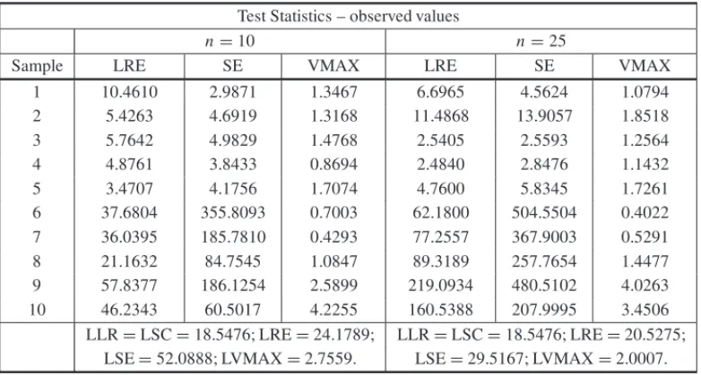
likelihood-ratio, the adapted Sullivan et al. and VMAX tests atα=0.005 significance level. The results are given in Tables 8 and 9 with the critical limits of each test considering the exact distribution as well as the asymptotic chi-square for the maximum likelihood-ratio and the adapted Sullivan et al. tests. For sample sizes ofn=5, the sample covariance matrices are also shown. By the exact distribution it can be seen that for the first 5 samples the null hypothesis was not rejected by any of the statistical tests and alln. For samples 6, 7, 8 and 9,H0was rejected by the adapted Sullivan
et al. (SE) test for all sample sizes; by the maximum likelihood-ratio (LRE) it was rejected for n = 10 and 25, except for sample 8 whose rejection occurred forn =25, only. On the other hand, VMAX rejected the null hypothesis only for sample 9 whenn =25 and did not rejected for samples 6, 7 and 8 for any sample size.
The null hypothesis was rejected for sample 10 by all statistical tests as expected considering the fact that this sample came from a multivariate normal distribution whose variance of X1is 3.2
Table 8– Results of the Example 2 – samples sizesn=10 andn=25 –α=0.005. Test Statistics – observed values
n=10 n=25
Sample LRE SE VMAX LRE SE VMAX
1 10.4610 2.9871 1.3467 6.6965 4.5624 1.0794 2 5.4263 4.6919 1.3168 11.4868 13.9057 1.8518 3 5.7642 4.9829 1.4768 2.5405 2.5593 1.2564 4 4.8761 3.8433 0.8694 2.4840 2.8476 1.1432 5 3.4707 4.1756 1.7074 4.7600 5.8345 1.7261 6 37.6804 355.8093 0.7003 62.1800 504.5504 0.4022 7 36.0395 185.7810 0.4293 77.2557 367.9003 0.5291 8 21.1632 84.7545 1.0847 89.3189 257.7654 1.4477 9 57.8377 186.1254 2.5899 219.0934 480.5102 4.0263 10 46.2343 60.5017 4.2255 160.5388 207.9995 3.4506
LLR=LSC=18.5476; LRE=24.1789; LLR=LSC=18.5476; LRE=20.5275; LSE=52.0888; LVMAX=2.7559. LSE=29.5167; LVMAX=2.0007.
(*) LLR and LSC: likelihood-ratio and the adapted Sullivan et. al tests critical limits using chi-square
distribution. LRE and LSE: likelihood-ratio and the adapted Sullivan et. al tests critical limits using exact
distribution. LVMAX: critical limit for VMAX test.
Considering the asymptotic chi-square distribution the null hypothesis was rejected for samples 6-10 by likelihood-ratio (LR) as well as by the adapted Sullivan et al. (SC) for all sample sizes. However, it is important to remind that as shown in Section 3.2, for p =3 andn =5, 10, 25, the type I error of these two tests for small samples is inflated being larger than the pre-specified significance level, particularly forn=5, 10.
It is interesting to point out that the same parametersµ0and0were used by Costa & Machado (2009), in the illustrative example given on Section 5 of their paper. The matrix1, which was used in our example, is the covariance matrix of the sample number 4 presented in Costa & Machado’s example (2009), and it was considered similar to the matrix0by the VMAX test in their paper.
5 FINAL REMARKS
Considering the exact distribution of the tests statistics, in the majority of the simulated cases, the adapted Sullivan et al. and the likelihood-ratio tests resulted in larger values of estimated power than VMAX for bivariate and trivariate normal distributions. VMAX was not sensitive to general changes in the covariance (or correlation) structure. Its estimated powers increased when the variances were larger under the alternative than the null hypothesis and the covariance (or correlation) structure remained similar underH0andH1. This result is no very surprising since
Table 9– Results of the Example 2 – sample sizen=5.
Sample covariance matrix Test statistic – Observed values
LRE SE VMAX
1 S1= ⎡
⎢ ⎣
0.0970 0.0419 0.0203 0.0419 0.0245 0.0123 0.0203 0.0123 0.0073
⎤
⎥
⎦ 5.8330 5.2599 1.9393
2 S2= ⎡
⎢ ⎣
0.0189 0.0012 0.0044 0.0012 0.0077 0.0069 0.0044 0.0069 0.0119
⎤
⎥
⎦ 5.4071 12.8939 1.0760
3 S3= ⎡
⎢ ⎣
0.0265 0.0176 0.0144 0.0176 0.0363 0.0158 0.0144 0.0158 0.0102
⎤
⎥
⎦ 11.4558 10.3729 1.5729
4 S4= ⎡
⎢ ⎣
0.0238 0.0007 0.0010 0.0007 0.0079 0.0069 0.0010 0.0069 0.0096
⎤
⎥
⎦ 4.5389 10.4866 0.7665
5 S5= ⎡
⎢ ⎣
0.0183 0.0128 0.0050 0.0128 0.0128 0.0049 0.0050 0.0049 0.0024
⎤
⎥
⎦ 12.0149 8.5493 0.7537
6 S6= ⎡
⎢ ⎣
0.0131 −0.0055 0.0019
−0.0055 0.0067 −0.0004 0.0019 −0.0004 0.0006
⎤
⎥
⎦ 23.6423 201.5283 0.2886
7 S7= ⎡
⎢ ⎣
0.0184 −0.0086 0.0015
−0.0086 0.0092 −0.0001 0.0015 −0.0001 0.0010
⎤
⎥
⎦ 19.4767 155.7951 0.4992
8 S8= ⎡
⎢ ⎣
0.0322 −0.0126 0.0027
−0.0126 0.0117 0.0000 0.0027 0.0000 0.0016
⎤
⎥
⎦ 20.3896 158.6873 1.2901
9 S9= ⎡
⎢ ⎣
0.0850 0.0039 0.0047 0.0039 0.0223 −0.0032 0.0047 −0.0032 0.0010
⎤
⎥
⎦ 33.6708 215.0552 3.0146
10 S10= ⎡
⎢ ⎣
0.3802 −0.0113 −0.0047
−0.0113 0.0175 0.0008
−0.0047 0.0008 0.0006
⎤
⎥
⎦ 79.7073 131.9005 7.6054
LLR=LSC=18.5476; LRE=36.4839; LSE=111.3334; LVMAX=3.8140 –α=0.005.
(*) LLR and LSC: likelihood-ratio and the adapted Sullivan et al. tests critical limits using chi-square
distribution. LRE and LSE: likelihood-ratio and the adapted Sullivan et. al tests critical limits using exact
distribution. LVMAX: critical limit for VMAX test.
The results presented in this paper had indicated that the adapted Sullivan et al. is a good al-ternative for testing hypothesis about the structure of the covariance matrix. It is a very flexible test and it can be applied in more general situations to detect differences in the variances as well as in other parameters of the covariance matrix. Also the fact that the adapted Sullivan et al. test depends upon the calculation of Fisher Information matrix, makes it possible to be used for multivariate normal and non-normal populations.
For small samples sizes the chi-square approximation did not performed well being not recom-mended since the estimates of type I error were larger than the pre-specified significance level for the adapted Sullivan et al. and for the likelihood-ratio tests. However, this fact does not make the use of the adapted Sullivan et al. or the likelihood-ratio tests restrictive since the exact dis-tribution of the respective test statistics under the null hypothesis are easily obtained by Monte Carlo simulation. The same is true for the VMAX test forp>2 since in these situations the use of numerical integration to find the critical region of the test is more complex and Monte Carlo simulation can be very helpful.
ACKNOWLEDGMENTS
This work was partially supported by the Brazilian Institutions CNPq and CAPES (PROCAD-Project). The authors wish to thank the anonymous referees for the suggestions that led to the improvement of the paper.
REFERENCES
[1] ALTF. 1985. Multivariate quality control. In:Encyclopedia of Statistical Sciences[edited by S. Kotz, & N.L. Johnson], vol. 6, John Wiley, 110–122.
[2] ANDERSONTW. 1958. An Introduction to Multivariate Statistical Analysis. New York: John Wiley & Sons, Inc.
[3] APARISIF, JABAIOYESJ & CARRIONA. 1999. Statistical properties of the|s|multivariate control chart.Communications in Statistics-Theory and Methods,28(11): 2671–2686.
[4] BEYERWH. 1978. Standard Mathematical Tables. West Palm Beach: CRC.
[5] CASELLAG & BERGERRL. 2002. Statistical Inference. California: Duxbury Thomson Learning.
[6] COSTA AFB & MACHADOMAG. 2009. A new chart based on sample variances for monitoring the covariance matrix of multivariate processes.International Journal of Advanced Manufacturing Technology,41(7-8): 770–779.
[7] COSTAAFB & MACHADOMAG. 2008. A new multivariate chart for monitoring the covariance ma-trix of bivariate processes.Communications in Statistics. Simulation and Computation,37(7): 1453– 1465.
[8] DAVISPJ & RABINOWITZP. 1984. Methods of Numerical Integration. Orlando: Academic Press.
[10] DJAUHARIMA. 2005. Improved monitoring of multivariate process variability.Journal of Quality Technology,37(1): 32–39.
[11] GARC´IA-DIAZJC. 2007. The effective variance control chart for monitoring the dispersion process with missing data.European Journal of Industrial Engineering,1(1): 40–55.
[12] JOHNSONRA & WICHERNWD. 2002. Applied Multivariate Statistical Analysis. New Jersey: Pren-tice Hall.
[13] LIY & TSUNGF. 2011. Detecting and diagnosing covariance matrix changes in multistage processes.
IIE Transactions,43(4): 259–274.x
[14] QUININOR, COSTAA & HOLL. 2012. A single statistic for monitoring the covariance matrix of bivariate processes.Quality Engineering,24(3): 423–430.
[15] MONTGOMERYDC. 2008. Introduction to Statistical Quality Control. New York: John Wiley.
[16] SULLIVANJH, STOUMBOSZG, MASONRL & YOUNGJC. 2007. Step-down analysis for change in the covariance matrix and other parameters.Journal of Quality Technology,39(1): 66–84. [17] YEHAB, LIB & WANGK. 2012. Monitoring multivariate process variability with individual
ob-servations via penalised likelihood estimation.International Journal of Production Research,50(22): 6624–6638.


![Figure 1 – Part of the example 2. Source: See [Aparisi et. al, 1999].](https://thumb-eu.123doks.com/thumbv2/123dok_br/18871283.420160/16.1063.290.708.152.461/figure-example-source-aparisi-et-al.webp)