DOI: http://dx.doi.org/10.1590/2446-4740.02617 Volume 33, Number 4, p. 331-343, 2017
Introduction
In spite of their simplicity, phenomenological models of spiking neurons have proved particularly useful in elucidating the dynamics of single neurons, as well as their role within large-scale neural networks. For instance, it was found that integrate-and-ire models with adaptation could predict the response of cortical neurons to somatically injected currents with high accuracy in spike timing (Brette and Gerstner, 2005; Jolivet et al., 2004; Kobayashi et al., 2009). An innovative alternative known as Neuroid (Prada et al., 2012) was introduced at the 34th International Annual Conference of the IEEE Engineering in Medicine and Biology Society
(EMBC’12). Since then, this neuron-model has been utilized to aid in understanding how functionally different neural populations (e.g., low-threshold vs. high-threshold afferent ibers; normally silent vs. tonically active neurons) interact each other and how those differences affect the way that visual (Prada et al., 2013) and tactile (Prada and Bustillos, 2013; Prada et al., 2015) information is processed.
The Neuroid is, indeed, one of the simplest neuron-models that have ever been conceived. It was built under the assumption that some neurons, under certain conditions, ire at regular rates when stimulation amplitude is held constant. The similarities between the action potential generation process and pulse frequency modulation (PFM) that have been pointed out by several authors (Bayly, 1968; Horch and Dhillon, 2004; Rieke et al., 1997) were also considered in building this neuron-model. It relies on a pair of heuristics that make possible to generate a spike train whose frequency is modulated by the amplitude of the stimulus (even though is widely known that the neuron iring rate may be affected by other factors, like the sub-threshold dynamics) and to demodulate the spike train in order to recover the modulating signal. But the real novelty of the Neuroid lies on what kind of experimental data is used to model different neural
The Neuroid revisited: A heuristic approach to model neural spike trains
Erick Javier Argüello Prada
1*, Ignacio Antonio Buscema Arteaga
2, Antonio José D’Alessandro Martínez
31 Department of Information Technology and Communications, Faculty of Engineering, Santiago de Cali University, Valle del Cauca, Colombia.
2 Departament of Technological, Biological and Biochemical Processes, Simón Bolívar University, Caracas, Venezuela. 3 Myocardial Contractility Laboratory, Institut of Experimental Medicine, Faculty of Medicine, Central University of Venezuela,
Caracas, Venezuela.
Abstract Introduction: Since it was introduced in 2012, the Neuroid has been used to aid in understanding how functionally different neural populations contribute to sensory information processing. However, insights about whether this neuron-model could perform better than others or about when its utilization should be considered have not been provided yet. Methods: In an attempt to address this issue, a comparison between the Neuroid and the leaky-integrate-and-ire (LIF) model in terms of accuracy and computational cost was performed. Both models were tested for different stimulation amplitudes and stimulation periods, with time step sizes ranging from 10-4 to 1 ms.
Results: It was found that, although the Neuroid was able to produce more accurate results than its original version, its accuracy was lower than the achieved with the LIF model solved by the forward Euler method. On the other hand, the Neuroid performed its calculations in an amount of time signiicantly lower (Mulfactorial ANOVA test, p < 0.05) than that required by the LIF model when it was solved by using the forward Euler method. Moreover, it was possible to use Neuroid-based networks to replicate biologically relevant iring patterns produced by low-scale networks composed of more detailed neuron-models. Conclusion: Results suggest that the Neuroid could be an interesting choice when computational resources are limited, although its use might be restricted to a narrow band of applications.
Keywords Neuroid, Spiking neuron-model, Frequency-intensity curve, Accuracy, Computational cost, Heuristic.
This is an Open Access article distributed under the terms of the Creative Commons Attribution License, which permits unrestricted use, distribution, and reproduction in any medium, provided the original work is properly cited.
How to cite this article: Prada EJA, Arteaga IAB, Martínez AJD. The Neuroid revisited: a heuristic approach to model neural spike trains. Res Biomed Eng. 2017; 33(4):331-343. DOI: 10.1590/2446-4740.02617. *Corresponding author: Departamento de Tecnologías de la Información y las Comunicaciones, Universidad Santiago de Cali, Calle 5 # 62-00 Barrio Pampalinda, Santiago de Cali, Valle del Cauca, Colombia. E-mail: [email protected]
populations. Instead of ionic conductances, equilibrium potentials and/or electrical membrane properties, the iring rate as a function of the stimulus intensity is the only requirement to build a Neuroid-based replica of the neuron under study. Essentially, the goal is to adjust the Neuroid’s parameters such that its frequency-intensity (F-I) curve resembles as much as possible the one that was built from experimental data. This novel approach, although simple in concept and application, may be little confusing for those who have already dealt with the
issues involved in using conductance-based neuron-models. Likewise, insights about whether this neuron-model could perform better than others or about when its utilization should be considered have not been provided so far.
Coordinated rhythmicity of neural populations may arise from the interaction of three aspects: the intrinsic properties of the cells composing the network, the synaptic properties of connections between neurons, and the topology of the network (Ermentrout and Terman, 2010). Speciically, the rhythm with which vertebrates and invertebrates walk, ly or swim, as well as communication based in stereotypically repeated visual or sound signals (e.g., the cricket song), is mostly driven by oscillatory patterns produced by neural networks of the central nervous system (Delcomyn, 1980). In order to study the mechanisms underlying this oscillatory activity, several authors (Friesen and Stent, 1977; Kling and Székely, 1968; Koch and Brunner, 1988) have used artiicial neurons, also known as “neuromimes”, built from elementary electronic components and able to provide a biologically plausible description of the neuron’s membrane. Nevertheless, it is unclear whether that activity is due to one of the above aspects, or to their combined action. Moreover, it is unknown whether oscillatory patterns produced by low-scale networks composed of highly detailed neuron-models can be replicated by Neuroid-based replicas of those networks.
In this sense, the present study aims: 1) to study how different sizes of time step affect the accuracy of the Neuroid, 2) to compare its performance to the exhibited by the leaky-integrate-and-ire (LIF) model in terms of accuracy and computational cost, and 3) to assess the feasibility in using Neuroid-based networks to replicate biologically relevant iring patterns produced by low-scale networks composed of much more detailed neuron-models.
Methods
Theoretical background
It is widely accepted that stimulus information (e.g., the intensity) is encoded not in the magnitude of a single spike but in the number of spikes ired per unit time
(iring rate). With that in mind, we think it would be appropriate to provide a mathematical representation of neural spike trains rather than investing time and effort in describing the action potential as an isolated event, as brilliantly done by Hodgkin and Huxley (Hodgkin and Huxley, 1952). Let us consider the triggering event s(t) given by:
( ) ( )
1
,
=
= ∑M j j j
s t w x t (1)
where x1, x2, …, xM are M normalized input signals and w1, w2, …, wM are their respective synaptic weights. Then, based on the fact that, under speciic conditions, some neurons can ire at a regular rate when the stimulus amplitude remains constant, the signal travelling along the neuron’s axon y(t) can be modeled as:
( ) 0 ( ) ( )
, 0
∞
=
∑δ − β >ϑ
= − ϑ
n
n T
t if s t
y t s t
otherwise
(2)
where δ(∙) represents a single spike, T denotes a constant with time units (necessary for dimensional consistency), ϑ is the relative threshold intensity and β is a proportionality constant that controls the slope of the Neuroid’s (F-I) curve. The Neuroid is also able to yield an amplitude-discrete version of s(t), named nt_out(t), by adjusting two additional parameters: Kr, a dimensionless constant which controls the output’s amplitude, and maxcount, a temporal parameter which allows to extend the output signal by several milliseconds after the last spike (Prada et al., 2012).
Even though it is not evident from the present study, each parameter of the Neuroid is inspired by a biological property of real neurons. For instance, the term ϑ represents the minimum stimulus intensity at which the neuron ires, at least, one action potential, and it has been deined in this way in order to be consistent with different stimulus types (thermal, mechanical, etc). The parameter β is associated to the potassium current lowing through the membrane, so the greater its value, the lower the slope of the F-I curve (Alberts et al., 2002; Koch and Brunner, 1988). The term maxcount denotes the time during which the neurotransmitter concentration is such that it has a synaptic effect in the cleft (Scimemi and Beato, 2009). Finally, although the parameter Kr does not have an obvious biological counterpart, its value depends on the iring frequency at the maximum amplitude of stimulation, which is calculated from the experimental F-I curve.
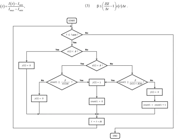
potential exceeds threshold, but also when the former reaches the latter (Matzner and Devor, 1992). To address this issue, the heuristic able to produce the signal y(t) (the Pulse Frequency Modulator in (Prada et al., 2012) was modiied such that the case in which the membrane potential reaches threshold was considered. Figure 1 shows a lowchart describing the new heuristic.
The accuracy of a neuron-model describes how reliable is the model in representing the behavior of biological neurons, in terms of the temporal resolution with which neural spikes can be produced (from miliseconds to fractions of miliseconds). Since simulating spiking neuron-models involves repeatedly solving the associated system of differential equations using analytical or numerical integration methods, the accuracy provided by such models may depends on, amongst other factors, the numerical method used to solve the system and the size of the time step Δt, an aspect that has not been explicitly mentioned and whose inluence has not been studied in previous implementations of our neuron-model.
Modeling approach
For each I ∈ [Imin, Imax], where Imin and Imax denote, respectively, the minimum and the maximum amplitudes of stimulation, there is an x ∈ [0, 1] given by:
( ) ( )= − ,
− min
max min
I t I x t
I I (3)
which represents one of the multiple inputs that may contribute to create the triggering event s(t), as expressed in Equation 1. As can be seen from Figure 1, if s(t) > ϑ, a spike is ired whenever the variable count1 reaches the smallest integer greater than or equal to the quantity
( )
(
s t β+ ϑ ∆)
t. Thus, the interspike interval (ISI) of the
spike train yielded by the Neuroid for a given s(t), can be calculated by using Equation 4:
( )
/ 1 ,
= β ∆ + ∆
ISI s t t t (4)
where the operator ⋅ denotes the ceiling function, which is deined as follows:
{ }
Z | 1 ,
= ∈ − < ≤
r min p p r p (5)
where r is a real number.
From Equation 5, it is clear that for all real number r we have:
. ≥
r r (6)
Therefore, from Equations 4 and 6, the value of the parameter β can be expressed as:
( )
1 .
β ≤ − ∆ ∆
ISI
s t t
t (7)
Figure 1. A novel heuristic, which, unlike the one originally proposed by Prada et al. (2012), considers the case in which membrane potential
Typically, the iring rate (f) of a single neuron is calculated by using Equation 8:
, = − spikes last first N f t t (8)
where Nspikes is the total number of spikes ired within the observation period while tirst and tlast are, respectively, the instants at which the irst and the last spike occur.
Interestingly, Equation 8 can be rewritten as:
(
)
, 1 = − spikes spikes avg N fN ISI (9)
where ISIavg represents the average interspike interval, which can be approximated to ISI when the neuron ires at a regular rate.
Finally, by identifying the iring rate of the neuron under study at the maximum amplitude of stimulation (fI_max), the interspike interval at that amplitude (ISII_max) is given by:
(
)
_ _ , 1 = − spikes I maxspikes I max
N ISI
N f (10)
which in turn allows us to rewrite Equation 7 to calculate the value of β required to model that neuron (note that s(t) = 1 at the maximum amplitude of stimulation):
_
1 .
β ≤ ∆ − ∆
I max
ISI
t
t (11)
Evaluating the Neuroid’s performance: iring
pattern and F-I curve
To evaluate the performance of a neuron-model, a benchmark solution (i.e., another model capable of providing a fairly good representation of neuronal behavior) is required. In our case, the benchmark solution was built by implementing the LIF model (Jolivet et al., 2004), which is commonly described by Equation 12:
( ) ( ) ( ), ( ) ( )
τm = rest− + m ≥ th → r
dV t
E V t R I t if V t V thenV t V
dt (12)
where V(t) is the membrane potential, I(t) is the input current, Erest is the resting membrane potential, Vth is the iring threshold, Vr is the after-spike membrane potential, Rm is the membrane resistance and τm is the membrane time constant. The LIF model was chosen as the benchmark solution because it has only a small number of parameters and it is one of the most computationally eficient spiking neuron-models, as reported in previous work (Long and Fang, 2010; Skocik and Long, 2014). In order to compute the parameters required to build a Neuroid-based replica of this “neuron”, Equation 12 was numerically solved by adopting the fourth-order Runge-Kutta method (RK4) with a time step Δt = 10-4 ms. The benchmark solution was implemented under MatLab 2013a using
Erest = 0 mV, Vth = 30 mV, Vr = -50 mV, Vspike = 70 mV, Rm = 8.22 MΩ, τm = 23.5 ms, and its F-I curve was built by increasing the amplitude of a rectangular current pulse I(t) applied during 1000 ms (the total time of run of each trial, denoted as tspan), from 0 to 20 nA (increments of 0.1 nA). The frequency was calculated by using Equation 8.
Once the F-I curve of the benchmark solution was built, the threshold intensity (Ith = 3.7 nA) and the iring rate at the maximum amplitude of stimulation (fI_max = 92.11 Hz) were identiied. Then, to build a Neuroid-based replica of that “neuron”, we found β from Equation 11 whereas ϑ was calculated by using Equation 13:
, − ϑ = − th min max min I I
I I (13)
where Ith is the threshold intensity.
Both the Neuroid (Δt = 10-4 ms) and the benchmark solution were run in MatLab 2013a for I = 3.7 nA (the threshold intensity) and I = 6 nA to compare their iring patterns at this two stimulation amplitudes. The same method used to calculate the iring rate of the LIF model, was used to calculate the iring rate achieved by the Neuroid. With time steps ranging from 10-4 to 1 ms, the F-I curve of the Neuroid was compared to the one previously built for the benchmark solution.
Accuracy and computational cost
Several methods have been used recently to evaluate the accuracy of a neuron-model. Wang and coworkers (Wang et al., 2014) totalized the number of false negatives (missed spikes) and false positives (additional or accidental spikes) with respect to the spike train generated by the HH neuron-model solved by the RK4 method, and then they divided each total by the number of matched spikes pairs to obtain two different indicators of accuracy. Skocik and Long (2014) estimated the accuracy of the LIF model, the HH model and the Izhikevich’s model (Izhikevich, 2003) by quantifying the absolute difference between the frequency of the model being tested (fmodel) and the frequency of its respective benchmark solution (fBM), which was taken to be the solution provided by the RK4 method with a time step of 10-4 ms, and then dividing the difference by the latter, as expressed in Equation 14:
( )
% =×model− BM 100.
BM
f f
Frequency Error
f
(14)
error deined by Skocik and Long (2014), except that this time the estimation was performed for three different stimulation amplitudes, taking into account the relative location of these amplitudes with respect to the dynamic range of the benchmark solution (i.e., the range of amplitudes for which it is able to ire, from Ith to Imax). Thus, three values were chosen: one slightly greater than the threshold intensity (I = 5 nA), one at the middle of the dynamic range (I = 12 nA), and one close to the maximum stimulation amplitude (I = 19 nA). For each, with a total time of run tspan = 1000 ms and with time steps ranging from 10-4 to 1 ms, we quantiied the frequency error produced by both the Neuroid and the LIF model solved by the Forward Euler (FE) method.
The interest in calculating the computational cost of a neuron-model arises from the assumption that the less computational power is required to simulate a single neuron, the easier it is to implement it into a large-scale neural network. According to several authors (Izhikevich, 2004; Long and Fang, 2010; Skocik and Long, 2014), a good indicator of how fast a neuron-model will perform its calculations is the number of loating point operations (FLOPs) required by the model. For a given time of run (tspan), the total of FLOPs required by a neuron-model can be estimated as follows:
( )( )
#= # ,
Total FLOPs FLOPs iterations (15)
where #FLOPs denotes the number of FLOPs per iteration and #iterations represents the total number of iterations for the given time of run:
# = . ∆ span t iterations t (16) The number of FLOPs per iteration depends mostly on the method used to determine if a spike can or cannot be ired. For instance, when the FE method is used to solve the LIF model (see Equation 12), the membrane potential is updated as follows:
( + ∆ =) ( )+
(
− ( )+ ( ))
∆ , τ rest m m tV t t V t E V t R I t (17)
which takes only 5 FLOPs by assuming that addition, multiplication, subtraction and division costs only one FLOP each, as done in previous studies (Izhikevich, 2004; Long and Fang, 2010; Skocik and Long, 2014). However, from Figure 1, it can be seen that, depending on whether the triggering input signal s(t) is less than, equal to or greater than the relative threshold intensity ϑ, the number of FLOPs per iteration may vary, as expressed in Equation 18:
( ) ( ) ( ) 0
2
# 3 , .
3 < ϑ = =
ϑ =
> ϑ
if s t
if a spikeis fired
FLOPs if s t where x
if no spikeis fired x if s t
(18)
This suggests that the total of FLOPs required by the Neuroid for a given time of run may decrease 1) when no stimulus is present, and 2) when iring rate increases. To test this hypothesis, we run both the Neuroid and the LIF model solved by the FE method under Dev-C++ 4.9.9.2, an integrated development environment for the C/C++ programming language, with time steps ranging from 10-4 to 1 ms. We used the FE method instead of the RK4 method because, even though the former is not the most accurate, it is one of the simplest numerical methods (Skocik and Long, 2014), which allowed us to perform a much more fair comparison. Wang et al. (2014) introduced a generalized exponential moving average method to solve a modiied version of the LIF model. Such method required a computation time lower than the required by the original LIF model and the HH model when they were solved by adopting the RK4 method. On the other hand, the utilization of the RK4 method for benchmarking clearly favored the method proposed by the group of Wang because the former is computationally expensive. Instead, we used a numerical method more affordable from a computational point of view in order to make a more fair comparison. The C++ programming language was used in calculating the computation time required by the Neuroid and the LIF model because it is possible to speed-up simulations up to several hundreds of times compared to MatLab (Andrews, 2012).
With time steps ranging from 10-4 to 1 ms, the LIF model and the Neuroid were run for three different simulation amplitudes (I = 5, 12 and 19 nA) and for three different stimulation periods (T = 200, 500 and 800 ms). The computation time required by each model was measured by using the QueryPerformanceCounter() function, and measurements were averaged over 10 repetitions. A factorial design was adopted by considering the neuron-model (LIF and Neuroid), the time step size, the stimulus amplitude and the stimulation duration as factors, each with 2, 5, 3 and 3 possible values or levels, respectively. Even though the analysis of the effects of interactions between factors on the computation time achieved by each model is beyond the scope of the present study, a multi-factor analysis of variance (ANOVA) was used to identify signiicant effects of each factor on the computation time (Montgomery, 2017). Values of p < 0.05 were considered statistically signiicant. Microsoft Excel 2010 (Microsoft Corporation, USA) and STATGRAPHICS Centurion XVI.I (version 16.1.18, Statistical Graphics Corporation) and Minitab 18 (ver 18.1, Minitab, Inc.) were used to perform the analysis.
Low-scale neural networks
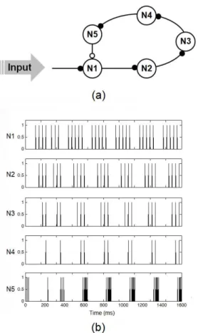
topology of the three-neuron oscillator and the “cricket song generator”, previously built by Koch and Brunner (1988) to test the neuron-model they developed. Neuroid-based replicas of the neurons modeled by Koch and Brunner were implemented under MatLab 2013a using ϑ = 0.2, β = 2.5, Kr = 3, maxcount = 24 and Δt = 0.1 ms for the three-neuron oscillator, and ϑ = 0.2, β = 2.5, Kr = 3, maxcount = 24 and Δt = 0.1 ms for the “cricket song generator”. As done in previous studies (Prada and Bustillos, 2013; Prada et al., 2012; 2013; 2015), synaptic coupling factors were taken to be equal to 1 or -1 in order to simulate, respectively, postsynaptic facilitation or inhibition. However, in the “cricket song generator”, neuron 4 strongly activates neuron 5, which in turn strongly inhibits neuron 1 (see section 3.2.4 in (Koch and Brunner, 1988)), so we empirically increased the coupling factors between these two pairs of neurons until the iring patterns of our Neuroid-based replica were as similar as possible to those obtained by Koch and Brunner. An Acer TravelMate B113, with an Intel Core i3-3217U and 4 GB of memory, was used to perform all simulations.
Results
The Neuroid can now ire at the threshold
intensity
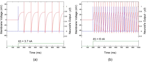
As shown in Figure 2, the Neuroid ired one single spike when the stimulation amplitude reached the threshold intensity (I = 3.7 nA), while the benchmark solution ired several spikes for the same stimulus. Both neuron-models showed a tonic response for I = 6 nA
and the total number of spikes produced by them were very similar.
The accuracy of the Neuroid improved when a time step of 10-2 ms or lower was used
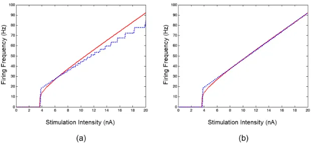
A comparison of the F-I curves for the Neuroid and the benchmark solution is shown in Figure 3. With a time step of 1 ms, discrepancies were observed between the responses produced by the Neuroid and the benchmark solution over the whole range of stimulation amplitudes. On the other hand, with a time step of 10-2 ms, the response of the Neuroid was in good agreement with that provided by the benchmark solution, except for a short range of amplitudes slightly greater than the threshold intensity (from 3.7 to 7 nA). It is worth noting that, as with many neuron-models, the iring frequency calculated by the Neuroid “jumped” to a non-zero value instead of increasing continuously at the threshold intensity. In fact, at this value, the Neuroid yielded f = 0 Hz and only for stimulation amplitudes greater than threshold our neuron-model yielded non-zero frequency values. This is because, to calculate the iring frequency, at least two spikes were required (see Methods). Since at the threshold intensity, only one spike was ired, the condition was not fulilled and the frequency was taken to be zero.
As it can be seen from Table 1, the Neuroid produced a iring frequency that approximates the one produced by the benchmark solution with an error less than 1%, using a time step less than or equal to 10-2 ms, except for I = 5 nA. Better results were obtained for the whole range of stimulation amplitudes by using the LIF model solved by adopting the FE method with a time step less than or equal to 10-1 ms.
Figure 2. The iring pattern of the Neuroid (Δt = 10-4 ms) and the benchmark solution (the LIF model solved by the fourth order Runge-Kutta method
The neuroid is signiicantly faster than the LIF
model solved by the FE method
From Figure 4 and Table 2, it can be seen that the mean computation time required by the Neuroid was signiicantly lower (Multifactorial ANOVA, p < 0.05) than the required by the LIF model when it was solved by using one of the simplest methods for approximating solutions to differential equations (i.e., the FE method). On the other hand, no signiicant differences were found in the computation time achieved by each model when different stimulation amplitudes and different stimulation periods were used (see Table 3).
Figure 5 shows, in the form of a Pareto chart, the absolute values of the standardized effects of each factor and all their possible combinations on the computation time required to calculate several hundreds of milliseconds of neural response. As can be seen, only the model (A) has a signiicantly and markedly effect on the computation time.
Neuroid-based networks can replicate the
iring patterns produced by short-scale
networks composed of more detailed units
Figures 6 and 7 show, respectively, the iring patterns produced by Neuroid-based replicas of both a three-neuron oscillator and the “cricket song generator”.
Figure 3. A comparison between the F-I curve of the Neuroid (blue dotted line) for two different time steps and the F-I curve of the benchmark
solution (red solid line). (a) When a time step of 1 ms was used, the Neuroid showed a poor agreement with the benchmark solution. (b) When a
time step of 10-2 ms (or lower) was used, the Neuroid showed a good agreement with the benchmark solution, except for a short range of amplitudes
slightly greater than the threshold intensity.
Table 1. Frequency errors for the LIF model (solved by the Forward Euler method) and the Neuroid at three different stimulation amplitudes
(I = 5, 12 and 19 nA) with time steps ranging from 10-4 to 1 ms. Values are expressed in percentages.
Time step Δt
(ms)
Stimulation amplitude (nA)
5 12 19
LIF Neuroid LIF Neuroid LIF Neuroid
100 0.94 9.16 0.84 9.09 3.80 11.10
10-1 0.14 11.65 0.25 1.34 0.51 1.36
10-2 0.00 11.89 0.02 0.78 0.01 0.26
10-3 0.00 11.94 0.00 0.73 0.01 0.11
10-4 0.00 11.94 0.02 0.73 0.00 0.10
Table 2. Summary of multiple range tests for computation time (the response
variable) by model. A multiple comparison procedure (the Fisher’s least
signiicant difference (LSD) procedure) was applied to determine which means are signiicantly different from which others. The bottom half of
the table shows the estimated difference between means. An asterisk has
been placed next to the pair showing a statistically signiicant difference at the 95% conidence level (LIF: leaky-integrate-and-ire; NEU: Neuroid).
Models Count LS Mean LS Sigma
Homogeneous groups
NEU 450 31.4092 1.50113 X
LIF 450 420.689 1.50113 X
Contrast Sig. Difference +/- Limits
LIF - NEU * 389.28 4.16085
In general, results are in good agreement with those obtained by earlier studies, in which more detailed neuron-models were used (Friesen and Stent, 1977; Kling and Székely, 1968; Koch and Brunner, 1988). Different oscillation frequencies can be achieved by the Neuroid-based replica of the three neuron oscillator by varying the stimulation amplitude (see Figure 6b), and the order in which neurons start iring is also preserved (N3 → N2 → N1 → N3). Although the Neuroid-based replica of the “cricket song generator” required a transition period of more than 400 ms in order to produce a iring pattern consistent with previous results (see Figure 7b), Neuroids 2, 3 and 4 start iring shortly after the second spike of the previous unit occurs, and the burst of spikes
generated by N5 produces a long-term pause in N1, in consistency with previous results (see Figure 10 in Koch and Brunner, 1988).
Discussion
Figure 2a shows that, unlike the benchmark solution, the Neuroid was able to ire a single spike when the stimulus amplitude reached the threshold intensity (I = 3.7 nA), which is consistent with the differences
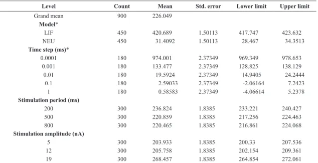
Table 3. Least-Squares Means for computation time with 95% conidence interval. Means, standard errors, lower and upper limits are expressed
in milliseconds. An asterisk has been placed next to the factor showing a statistically signiicant difference between means at the 95% conidence level (LIF: leaky-integrate-and-ire; NEU: Neuroid).
Level Count Mean Std. error Lower limit Upper limit
Grand mean 900 226.049
Model*
LIF 450 420.689 1.50113 417.747 423.632
NEU 450 31.4092 1.50113 28.467 34.3513
Time step (ms)*
0.0001 180 974.001 2.37349 969.349 978.653
0.001 180 133.477 2.37349 128.825 138.129
0.01 180 19.5924 2.37349 14.9405 24.2444
0.1 180 2.59033 2.37349 -2.06164 7.2423
1 180 0.58583 2.37349 -4.06614 5.2378
Stimulation period (ms)
200 300 236.824 1.8385 233.221 240.427
500 300 220.859 1.8385 217.256 224.463
800 300 220.465 1.8385 216.861 224.068
Stimulation amplitude (nA)
5 300 203.933 1.8385 200.33 207.536
12 300 205.758 1.8385 202.154 209.361
19 300 268.457 1.8385 264.854 272.061
*This factor shows signiicant differences at the 95% conidence level.
Figure 4. Least-Squares means of the computation times achieved by
the LIF model (FE method) and the Neuroid. Both models were run for
three different simulation amplitudes (I = 5, 12 and 19 nA) and for three different stimulation periods (T = 200, 500 and 800 ms), with time steps ranging from 10-4 to 1 ms.
Figure 5. Absolute values of the standardized effects of each factor and
all their possible combinations on the computation time. Only the model (A) has a signiicative and markedly effect on the computation time
between the conditions required for the propagation of single spikes and those required for spike train generation (when sustained depolarizing pulses are applied at progressive increasing intensities, a “threshold intensity” is reached at which one single spike is ired... only when the stimulus intensity becomes higher, a spike train is produced) (Matzner and Devor, 1992). However, the response shown in Figure 2a cannot be assumed to be a phasic response, which include not only those exhibiting one single spike at the onset of the stimulus, but also those showing brief spike trains starting during the beginning of the stimulation period (Madrid et al., 2003; Mitra and Miller, 2007; Ruscheweyh and Sandkühler, 2002). In fact, the absence of a delay in spike iring at different stimulus intensities shows a fundamental limitation of our neuron-model and the assumption on which the model relies is, indeed, an oversimpliication of the neural behavior because only some neurons ire at a regular frequency when stimulation amplitude is held constant and they do only under certain conditions.
Figure 6. A three-Neuroid oscillator. (a) The oscillator consists of three
neurons simultaneously receiving a constant excitatory input (●), while they are cyclically connected through inhibitory synapses (○). (b) Firing
patterns obtained by the authors for three different simulation intensities
(Input = 5, 3 and 2.7 μA) after implementing a Neuroid-based replica
of the three-neuron oscillator.
Figure 7. Using the Neuroid to build the “cricket song generator”.
(a) Neuron 1 receives a constant excitatory input, which is transmitted
to neurons 2, 3, 4 and 5 through excitatory synapses (●), while neuron 5 provides neuron 1 with strong inhibition (○). (b) Firing patterns
obtained by the authors after implementing a Neuroid-based replica of
The Neuroid does not account for the dynamics of the voltage-dependent membrane conductances that are responsible for the generation of action potentials, which is why spike trains show no clear threshold dependence or temporal behavior consistent with the latencies of ionic channels (see Figure 2b). Small differences in the membrane voltage are a great concern for several neural phenomena, such as spike-timing-dependent plasticity (STDP) (Dan and Mu-ming, 2004; Shulz and Feldman, 2013), so the use and value of our neuron-model might be limited to a narrow band of applications.
While the Neuroid is now able to produce more accurate results when a time step of 10-2 ms or lower is used, its accuracy is considerably lower than the achieved with the LIF model solved by the FE method (see Table 1). The latter is consistent with the result obtained during a previous study (Skocik and Long, 2014), in which it was shown that the LIF model provides fairly accurate results when the FE method with a time step of 0.1 ms or lower is used. On the other hand, that comparison was carried out not between models but between numerical methods because, by deinition, the iring frequency produced by one model is different from the iring frequency produced by the others. More reliable results could be obtained if the iring rate of the model is compared to the iring rate of a biological neuron. Still, this comparison would be a bit more complicated since the neural response varies between different populations. A previous study (Prada et al., 2015) found that the Neuroid might be used to predict the iring frequency of nociceptive primary afferent A- and C-ibers, but it could be insuficient to model spinal dorsal horn neurons. All this suggests that, in the absence of a quantitative index for the evaluation of the accuracy achieved by several neuron-models, the results obtained by previous (Izhikevich, 2004; Long and Fang, 2010; Skocik and Long, 2014; Wang et al., 2014) and the current study may not be absolutely conclusive.
From Figures 4 and 5, and Tables 2 and 3, it is clear that the computation time required by the Neuroid is signiicantly lower (Multifactorial ANOVA, p < 0.05) than the required by the LIF model when it is solved by using the FE method, which is one of the simplest methods for approximating solutions to differential equations (Izhikevich, 2004; Skocik and Long, 2014). In general, the Neuroid performs its calculations in an amount of time signiicantly lower than the required by the LIF model, under the same conditions. Surprisingly, such differences do not increase signiicantly either when the stimulation amplitude increases or the stimulation period decreases (see Table 3). Even so, it is worth noting that the FLOPs per iteration required by the Neuroid decreases by one whenever a spike is ired, since the variable count1 is reset instead of increasing by one when its value reaches or exceeds the quantity
( )
(
s t β+ ϑ ∆)
t (see Figure 1). Thus, as the stimulationamplitude increases and, therefore, the iring frequency, the total of FLOPs required for a given time of run decreases. Additionally, no operation is executed in the absence of stimulus because the Neuroid irst compares the triggering event to the activation threshold and only if the former reaches or exceeds the latter, the model performs its calculations. On the contrary, classic neuron-models irst update the membrane potential in terms of their parameters and the stimulus amplitude (even in the absence of stimulus), and then compare the resulting potential to the activation threshold, after which a spike can or cannot be ired (Gerstner et al., 2014). The ideas above are summarized in Figure 8.
This “compare irst, calculate later” feature makes the Neuroid an attractive option for those who want to model the behavior of large-scale neural networks through which the information is transmitted in the form of short-duration pulses (e.g., Spiking Neural Networks), especially when computational resources are limited, since its computational cost is signiicantly lower than the one required by the legendary LIF model. For instance, about one third to 40% of the cortical neuron population is composed by neurons capable of iring extremely narrow spikes at a very high frequency (300-400 Hz) with a very low adaptation rate (Wang et al., 2016), precisely the kind of behavior that the Neuroid is able to reproduce. However, it must be taken into account that the computational cost of a neuron-model tends to increase with its accuracy, which in turn depends on, among other factors, the size of the time step. Nowadays, it is possible to implement some alternatives, like the one proposed by Wang et al. (2014), whose accuracy is not signiicantly affected by the time step size. Yet, and as we previously pointed out, results reported by that and other studies should be analyzed in the light of a common quantitative index of a neuron-model’s accuracy, which may lead to a more objective comparison.
neuron connectivity and/or the topology of the network. Therefore, it would be possible to use Neuroids in analyzing to what extent emergent properties derived from mutual connectivity between neurons contribute to the generation of bursting oscillatory patterns. Neuroid-based replicas of some biological neural networks, whose architecture is well known, might be built and studied before using much more detailed simulation tools or packages. This, in turn, demands an accurate identiication of the cells composing those networks as well as a wiring diagram describing how they are connected, which may lead to new research opportunities. Lastly, a result like this could be viewed as a small extension of the Hopield’s work (Hopfield, 1984; 1982), in which it was found that the computational properties of networks composed of binary unrealistic units, like the McCulloch and Pitts model (McCulloch and Pitts, 1943), are often preserved in networks composed of units having continuous input-output relationships and integrative time delays.
Like any heuristic, the Neuroid does not guarantee an optimal solution for a wide range of problems. Our neuron-model is, indeed, far from being a biologically meaningful model, since the conditions and assumptions upon which the model was formulated are very speciic. It is widely known that the iring rate of real neurons depends not only on the stimulation intensity, but also on several other factors like subthreshold dynamics, a feature which our neuron-model fails to exhibit. On the other hand, and according with results presented before, the Neuroid requires a smaller amount of computational resources than those required by the LIF model to simulate several hundreds of milliseconds of neuronal response under the same conditions. This suggests that the Neuroid may be an interesting option for the implementation of networks through which the information is transmitted in the form of short-duration pulses (e.g., Spiking Neural Networks), especially when computational resources are limited. Furthermore, the low computational cost required by the Neuroid, as well as its lexibility to be adapted to any type of programming language (C ++, MATLAB, HPVEE, LabVIEW) make it suitable for the development of free and open computational tools based on Neuroids, as the one developed in the University of Guayaquil (Silva Muñoz, 2015). Future work may include considering the noise inluence by adding a probabilistic component to the Neuroid without altering its low computational requirement.
The fact that our neuron-model is able to reproduce only a few neuro-computational properties could make it a useful tool for determining if the iring patterns exhibited by neurons composing certain networks are due to the intrinsic properties of these cells, or to the topology of the network. In other words, if a Neuroid-based replica is able to reproduce the iring patterns observed in a
biological network, then these patterns are likely to be produced by the interactions between different cells or nodes. This indeed underlines the importance of neural connection for the generation of speciic iring patterns, and also demands an accurate identiication of the cells composing those networks as well as a wiring diagram describing how they are connected, which may lead to new research opportunities.
As a concluding remark, beyond a simple comparison between different average iring rates or coincident spikes, researchers and modelers still lack a standardized set of tests to quantify and compare the accuracy of distinct neuron-models, so further work is needed to provide these communities with a common framework that can be used as a reference for this purpose.
Acknowledgements
The authors thank Prof. Minaya Villasana for her valuable ideas and useful observations during the realization of this article.
References
Alberts B, Johnson A, Lewis J, Raff M, Roberts K, Walter P. Molecular biology of the cell. 4th ed. New York: Garland Science; 2002.
Andrews T. Computation time comparison between Matlab snd C++ using Launch Windows. Aerosp Eng. 2012; 78:1-6. Bayly EJ. Spectral analysis of pulse frequency modulation in the nervous systems. IEEE Trans Biomed Eng. 1968; 15(4):257-65. PMid:5699902. http://dx.doi.org/10.1109/ TBME.1968.4502576.
Brette R, Gerstner W. Adaptive exponential integrate-and-fire model as an effective description of neuronal activity. J Neurophysiol. 2005; 94(5):3637-42. PMid:16014787. https:// doi.org/ 10.1152/jn.00686.2005.
Dan Y, Mu-ming P. Spike timing-dependent plasticity of neural circuits. Neuron. 2004; 4(1):23-30. https://doi.org/10.1016/j. neuron.2004.09.007.
Delcomyn F. Neural basis of rhythmic behavior in animals. Science. 1980; 210(4469):492-8. PMid:7423199. http://dx.doi. org/10.1126/science.7423199.
Ermentrout GB, Terman DH. Mathematical foundations of neuroscience. Vol. 35. New York: Springer Science & Business Media; 2010.
Friesen WO, Stent GS. Generation of a locomotory rythm by a Neural Network with Recurrent Cyclic Inhibition. Biol Cybern. 1977; 28(1):27-40. PMid:597508. http://dx.doi. org/10.1007/BF00360911.
Gerstner W, Kistler WM, Naud R, Paninsky L. Neuronal dynamics: from single neurons to networks and models of cognition. Cambridge: University Press; 2014.
nerve. J Physiol. 1952; 117(4):500-44. PMid:12991237. http:// dx.doi.org/10.1113/jphysiol.1952.sp004764.
Hopfield JJ. Neural networks and physical systems with emergent collective computational abilities. Proc Natl Acad Sci USA. 1982; 79(8):2554-8. PMid:6953413. http://dx.doi. org/10.1073/pnas.79.8.2554.
Hopfield JJ. Neurons with graded response have collective computational properties like those of two-state neurons. Proc Natl Acad Sci USA. 1984; 81(10):3088-92. PMid:6587342. http://dx.doi.org/10.1073/pnas.81.10.3088.
Horch KW, Dhillon GS. Neuroprosthetics: theory and practice. New York: World Scientific; 2004.
Izhikevich EM. Simple model of spiking neuron. IEEE Trans Neural Netw. 2003; 14(6):1569-72. PMid:18244602. https:// doi.org/10.1109/TNN.2003.820440.
Izhikevich EM. Which model to use for cortical spiking neurons? IEEE Trans Neural Netw. 2004; 15(5):1063-70. PMid:15484883. https://doi.org/10.1109/TNN.2004.832719. Izhikevich EM. Dynamical systems in neuroscience: the geometry of excitability and bursting. Cambridge: MIT Press; 2007. Jolivet R, Lewis TJ, Gerstner W. Generalized integrate-and-fire models of neuronal activity approximate spike trains of a detailed model to a high degree of accuracy. J Neurophysiol. 2004; 92(2):959-76. PMid:15277599. https://doi.org/10.1152/ jn.00190.2004.
Kling U, Székely G. Simulation of rhythmic nervous activities. I. Function of networks with cyclic inhibitions. Kybernetik. 1968; 5(3):89-103. PMid:5728516. http://dx.doi.org/10.1007/ BF00288899.
Kobayashi R, Tsubo Y, Shinomoto S. Made-to-order spiking neuron model equipped with a multi-timescale adaptive threshold. Front Comput Neurosci. 2009; 3:9. PMid: 19668702. https:// doi.org/10.3389/neuro.10.009.2009.
Koch UT, Brunner M. A modular analog neuron-model for research and teaching. Biol Cybern. 1988; 59(4-5):303-12. PMid:3196775. http://dx.doi.org/10.1007/BF00332920.
Krahe R, Gabbiani F. Burst firing in sensory systems. Nat Rev Neurosci. 2004; 5(1):13-23. PMid:14661065. http://dx.doi. org/10.1038/nrn1296.
Long L, Fang G. A review of biologically plausible neuron models for spiking neural networks. In: Proceedings of the AIAA InfoTech@ Aerosp Conference; 2010 Apr 20-22; Atlanta, GA. Atlanta: AIAA; 2010. http://dx.doi.org/10.2514/6.2010-3540. Madrid R, Sanhueza M, Alvarez O, Bacigalupo J. Tonic and phasic receptor neurons in the vertebrate olfactory epithelium. Biophys J. 2003; 84(6):4167-81. PMid:12770919. https://doi. org/10.1016/S0006-3495(03)75141-8.
Matzner O, Devor M. Na+ conductance and the threshold for repetitive neuronal firing. Brain Res. 1992; 597(1):92-8. PMid:1335824. http://dx.doi.org/10.1016/0006-8993(92)91509-D. McCulloch WS, Pitts WH. A logical calculus of the ideas immanent in nervous activity. Bull Math Biol. 1943; 5(4):115-33. https://doi.org/ 10.1007/BF02478259.
Mitra P, Miller RF. Normal and rebound impulse firing in retinal ganglion cells. Vis Neurosci. 2007; 24(1):79-90. PMid:17430611. https://doi.org/10.1017/S0952523807070101. Montgomery DC. Design and analysis of experiments. Hoboken: John Wiley & Sons; 2017.
Prada EJA, Bustillos RJS, Huerta MK, Martínez ADA. Lamina specific loss of inhibition may lead to distinct neuropathic manifestations: a computational modeling approach. Res Biomed Eng. 2015; 31(2):133-47. http://dx.doi.org/10.1590/2446-4740.0734.
Prada EJA, Bustillos RJS, Castillo C, Huerta M. New trends in computational modeling: a neuroid-based retina model. In: Proceedings of the 35th Annual International Conference IEEE Engineering in Medicine and Biology Society; 2013 Jul 3-7; Osaka, Japan. Osaka: IEEE; 2013. p. 4561-4. PMid: 24110749. https://doi.org/10.1109/EMBC.2013.6610562.
Prada EJA, Bustillos RJS, Castillo C, Huerta M. The neuroid: a novel and simplified neuron-model. In: Proceedings of the 34th Annual International Conference IEEE Engineering in Medicine and Biology Society; 2012 Aug 28-Sep 1; San Diego, CA. San Diego: IEEE; 2012. p. 1234-7. PMid:23366121. https://doi.org/10.1109/EMBC.2012.6346160.
Prada EJA, Bustillos RJS. The implementation of the Neuroid in the gate control system leads to new ideas about pain processing. Rev Bras Eng Bioméd. 2013; 29(3):254-61. http:// dx.doi.org/10.4322/rbeb.2013.025.
Rieke F, Warland D, van Steveninck RR, Bialek W. Spikes: exploring the neural code. Cambridge: MIT Press; 1997. Ruscheweyh R, Sandkühler J. Lamina-specific membrane and discharge properties of rat spinal dorsal horn neurones in vitro. J Physiol. 2002; 541(1):231-44. PMid:12015432. http:// dx.doi.org/10.1113/jphysiol.2002.017756.
Silva Muñoz AM. Desarrollo de un software para la construcción de redes neuroidales [thesis]. Guayaquil-Ecuador: Universidad de Guayaquil; 2015.
Scimemi A, Beato M. Determining the neurotransmitter concentration profile at active synapses. Mol Neurobiol. 2009. 40(3):289-306. https://doi.org/ 10.1007/s12035-009-8087-7. Shulz DE, Feldman DE. Spike timing-dependent plasticity. In: Rubenstein JLR, Rakic P. Comprehensive developmental neuroscience: neural circuit development and function in the healthy and diseased brain. San Diego, CA: Elsevier; 2013. p. 155-81.
Skocik MJ, Long LN. On the capabilities and computational costs of neuron models. IEEE Trans Neural Netw Learn Syst. 2014; 25(8):1474-83. PMid: 25050945. https://doi.org/10.1109/ TNNLS.2013.2294016.
Wang Z, Guo L, Adjouadi M. A generalized Leaky Integrate-and-Fire neuron model with fast implementation method. Int J Neural Syst. 2014; 24(5):1440004. PMid:24875788. http:// dx.doi.org/10.1142/S0129065714400048.