ISSN 0101-8205 www.scielo.br/cam
On the statistical steady state gas-solid flow in a riser
as predicted through a two-fluid simulation
CHRISTIAN C. MILIOLI and FERNANDO E. MILIOLI
Thermal and Fluids Engineering Laboratory
EESC – School of Engineering of São Carlos, USP – University of São Paulo Av. Trabalhador São-Carlense, 400, 13566-590 São Carlos, SP, Brazil
E-mails: [email protected] / [email protected]
Abstract. This work is concerned with the extremely high computational costs of the
two-fluid simulations of gas-solid flows in risers. In a previous article [1] a procedure was proposed
to speed up the simulations towards the desired statistical steady state flow regime. In this
con-tinuing article the concern is turned to the time extent that a simulation must advance inside the
statistical steady state regime so that suitable time averaged predictions can be made. An analysis
is carried out using the results of a transient two-fluid simulation of a riser flow performed inside
the statistical steady state regime. Time averaged results were produced considering different time
averaging intervals of 5, 10, 15 and 20 seconds. Both the transient behavior of the predictions
and the time averaged results are discussed. For the present case, it was found that 10 seconds of
fluidization taken inside the statistical steady state regime are enough for a reasonable qualitative
description of the average flow.
Mathematical subject classification: Primary: 06B10; Secondary: 06D05.
Key words:two-fluid simulation, gas-solid flow, circulating fluidized bed, riser.
1 Introduction
Circulating fluidized bed reactors are widely used in large scale applications such as catalytic cracking of petrol and coal combustion. Development and
design in those areas are strongly based on demonstration plants, at extremely high costs. In this context, treatments applying computational fluid mechanics assume considerable relevance. The complex gas-solid flow patterns which de-velop inside the risers of circulating fluidized bed reactors determine reaction rates, so that rigorous hydrodynamic descriptions are required. The continuum Eulerian or two-fluid models are currently considered the most practical choice for providing such descriptions [2].
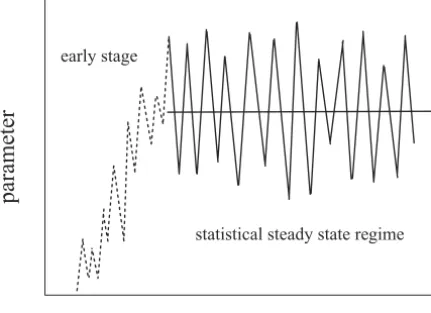
Owing to flow instabilities, the risers can not operate in real steady state condi-tions. Instead, they operate in pseudo-permanent or statistical steady state flow regimes, imposing numerical simulations to be transient. Figure 1 illustrates the behavior of any parameter as predicted from a two-fluid transient simula-tion of the gas-solid flow in risers (see [3], for instance). From a given initial condition, the simulation goes through an early stage, and finally reaches the so called statistical steady state regime. For practical purposes, this regime is considered to be reached when all the flow parameters start to oscillate around well defined averages.
early stage
statistical steady state regime
pa
ra
m
et
er
time
Figure 1 – Behavior of any parameter as predicted from a two-fluid transient simulation.
regime [3-8]. None of those works performed any analysis on the averaging time interval that would be required for obtaining suitable averaged results. Tsuo and Gidaspow [8] generated time averaged results considering only 5 seconds of real fluidization inside the statistical steady state regime, Zhang and Vander-Heyden [7] considered 10 to 15 seconds, Mathiesen et al. [6] considered 16 to 20 seconds, and Cabezas-Gómez and Milioli [5] considered 80 seconds.
discussion is carried out on the independence of the averaged results regarding the averaging time interval. The present simulation was performed in a 10 nodes Beowulf cluster of PCs, each one with 2 processors Intel Xeon 3.06 GHz and 20 Gb Ram, totalizing 122.4 Gflops of computing capacity.
2 Two-fluid modeling of gas-solid flow
each phase. In the second formulation, conservative equations are generated for the gas phase and for the mixture. From those equations, conservative equa-tions are derived for the solid phase. Gidaspow [11] named those formulaequa-tions as models A and B, respectively. The formulation of model A, which is used in this work, is showed next.
Gas phase continuity:
∂(αgρg)
∂t +
− →
∇ ∙(αgρg
−→
Ug)=0 (1)
Solid phase continuity:
∂(αsρs)
∂t +
− →
∇ ∙(αsρs
− →
Us)=0 (2)
Gas phase momentum:
∂(αgρg
−→
Ug)
∂t +
− →
∇ ∙(αgρg
−→
Ug
−→
Ug)=
−−→∇(αgPg)+
− →
∇ ∙(αgτg)+αgρg
− →
Fg+β(
− →
Us −
−→
Ug)
(3)
Solid phase momentum:
∂(αsρs
− →
Us)
∂t +
− →
∇ ∙(αsρs
− →
Us
− →
Us)=
−−→∇(αsPs)+
− →
∇ ∙(αsτs)+αsρs
− →
Fs −β(
−→
Us −
− →
Ug)
(4)
Stress tensor for phasek:
τk =μk[
− →
∇U−→k+(
− →
∇−→Uk)T] +λk(
− →
∇ ∙−→Uk)I (5)
where,μk =constant, λk = 23μk.
Solid phase pressure [13]:
− →
∇(αsPs)= −
− →
∇αs+
− →
∇(αsPg) (6)
where,
Volumetric continuity:
αg+αs =1 (8)
External body forces per unit mass:
− →
Fg =−→g (9)
−→
Fs =
ρs −ρg
ρs
−
→g (10)
Equations of state: ρg=constante, ρs =constante.
Interface drag [11]:
β =150 α
2
sμg
αg(dpϕs)2
+1.75ρgαs|vg−vs|
(dpϕs)
for αs >0.2 (11)
β = 3
4CDs
ρgαsαg|vg−vs|
(dpϕs)
α−g2.65 for αs ≤0.2 (12)
where:
CDs =
24
Rep 1+0.15 Re0p.687
for Rep<1000 (13)
and
CDs =0.44 Rep ≥1000 (14)
with
Rep =
|vg−vs|dpρgαg
μg
(15)
The symbols in Equations (1) to (15) stand for: CD – drag coefficient,
non-dimensional; dp – particle diameter, m;
− →
F – external body force per unit mass, N;−→g – gravity acceleration, m/s2; I – unit tensor; P – pressure, N/m2; Rep – Reynolds number, non-dimensional; t – time, s;
− →
U – average velocity vector, m/s; u, v, w – velocity components in the directions, m/s; α – vol-ume fraction, m3k/m3; β – gas-solid friction coefficient, kg/m3s; ϕs – particle
Equations (11), (12), and (13)-(14) are due to Ergun [14], Wen and Yu [15] and Rowe [16], respectively. The complex set of partial differential non-linear coupled equations of the two-fluid models can only be solved through numer-ical procedures. In this work, the numernumer-ical model available in the software CFX [17-19] is used. An element-based finite volume discretization method is followed. Non-structured meshes are applied in Cartesian coordinate system. Tetrahedral mesh elements are used. The median method is applied to define control volumes over which the conservative equations are integrated to obtain the discretized equations. The discretization of convective terms are performed through a second order high resolution interpolation scheme. The discretiza-tion of diffusive and other terms is performed through the second order central differencing scheme. Time discretization is performed through a first order in-terpolation scheme. The discretized equations are solved implicitly through a direct method applying matrix inversion. As a consequence, couplings such as pressure× velocity, and drag, are straightly solved, and iteration is only re-quired to overcome non-linearities.
3 Simulation
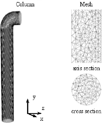
The present simulation was performed for hydrodynamic conditions which have already been considered by other authors, and are typical of circulating fluidized bed coal combustion. The solid mass flux of 24.9 kg/m2s, particulate size of 520μm, and the reactor size (height of 5.56 m and width of 7.62 cm) were taken from Luo [20]. Figure 2 shows the three-dimensional cylindrical geome-try that was assumed, and a sample of the numerical mesh that was applied.
Table 1 brings fluid and particulate properties, initial and boundary condi-tions, and numerical settings. The dynamic viscosity of the solid phase of 0.509 N/m2s was determined by Tsuo [21] using the empirical data of Luo [20].
4 Results and Discussion
Figure 2 – Geometry and a sample of the tetrahedral numerical mesh.
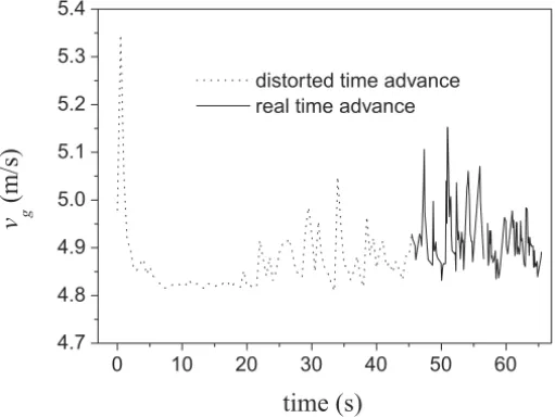
The results stand for the transient behavior of the gas and solid axial veloci-ties, solid mass flux and solid volume fraction, averaged over the cross section at 3.4 m above entrance. The distorted time predictions were allowed to proceed up to 45.454 seconds of distorted time fluidization. All the graphs show that, from about 20 seconds of distorted time fluidization, the predictions were already oscillating around well defined time averages, indicating that the early stage of the simulation was overcome.
Following the 45.454 seconds of non-converged distorted results, 20 seconds of real time predictions are presented, which are converged inside a rms (root mean square) of 1×10⁻⁵s.
Column
Diameter=7.62 cm Height=5.56 m
Particulate size=520μm Solid mass flux(Gs)=24.9 kg/m2s
Phases
g=air at 300 K s =glass beads at 300 K
Properties
ρg=1.1614 kg/m3 ρs =2620 kg/m3
μg =1.8210−5N/m2s μs =0.509 N/m2s
Wg =28.97 kg/kmol Ws =60 kg/kmol
Boundary conditions
Inlet
ug=0 m/s us =0 m/s
vg=4.979 m/s vs =0.386 m/s
wg =0 m/s ws =0 m/s
αg=0.9754 m3g/m3 αs =0.0246 m3s/m3
outlet walls
Locally parabolic g= no-slip
Pg=15880 N/m2 s = free-slip
Initial conditions (distorted time run)
As in the inlet, except:
αg=0.62 m3g/m
3 α
s =0.38 m3s/m 3 Numerical settings
Mesh
Tetrahedrals =206229
Average edge length =9.4 mm
Nodes =42029
rms for convergence =1×10⁻⁵s Distorted time step =1×10⁻³s
Real time step =1×10⁻⁴s
0 10 20 30 40 50 60 4.7
4.8 4.9 5.0 5.1 5.2 5.3 5.4
v g
(m
/s
)
time (s)
distorted time advance real time advance
Figure 3 – Transient behavior of the gas axial velocity averaged over the cross section at 3.4 m above entrance, for the distorted time simulation followed by the real time simulation.
0 10 20 30 40 50 60
-1 0 1 2 3 4
v
s(m
/s
)
time (s)
distorted time advance real time advance
0 10 20 30 40 50 60 -400
-200 0 200 400 3600 3800 4000
24.9
G
s(kg
s
/m
2
s)
time (s)
distorted time advance real time advance
Figure 5 – Transient behavior of the solid mass flux averaged over the cross section at 3.4 m above entrance, for the distorted time simulation followed by the real time simulation.
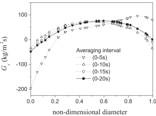
Time averaged results were generated for the predictions inside the statistical steady state region, considering different averaging intervals. Those were 0-5, 0-10, 0-15, and 0-20 seconds. Figures 7 to 10 show those results, which are time averaged profiles of gas and solid axial velocities, solid mass flux and solid volume fraction, through the diameter of the column, in the cross section at 3.4 m above entrance. Time averaged results in vertical risers are expected to be symmetric. The only possible cause for asymmetry, in the present case, concerns the asymmetric exit section. As the exit is very far away from the section where the results are analysed, it could be argued that only slight asymetries should be observed. However, the formation of clusters at the walls close to the exit, and the following down flow along the walls resulted highly affected by the asym-etric exit, accounting for the asymmasym-etric profiles reported in Figures 7 to 10.
For all of the concerning parameters, it is seen that the time averaging inter-val significantly affected the averaged predictions as well as the symmetry of the profiles. The differences were not only quantitative, but also qualitative. This is particularly clear for the profiles of solid mass flux showed in Figure 9. For the time interval (0-5s) the profile resulted quite asymmetric, unlike the nearly symmetric profiles obtained for the intervals (0-10s), (0-15s) and (0-20s).
0.0 0.2 0.4 0.6 0.8 1.0
0 2 4 6 8
v
g(m
/s
)
non-dimensional diameter
Averaging interval (0-5s) (0-10s) (0-15s) (0-20s)
0.0 0.2 0.4 0.6 0.8 1.0 -1
0 1 2
v
s(m
/s
)
non-dimensional diameter
Averaging interval (0-5s) (0-10s) (0-15s) (0-20s)
Figure 8 – Time averaged profiles of solid axial velocity through the diameter of the column, in the cross section at 3.4 m above entrance, for different time intervals.
It was expected that the profiles for all of the parameters became closer as the time averaging interval was raised.
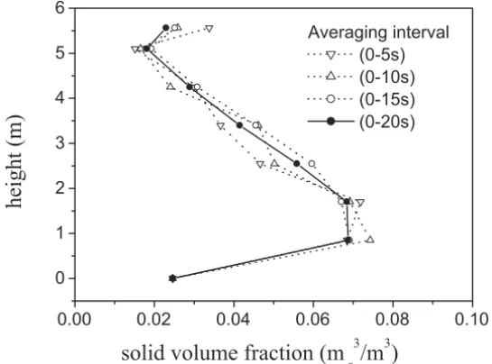
This, however, only happened for some of the parameters (solid mass flux and volume fraction). Otherwise, for each one of the parameters, the profiles presented the same qualitative behavior for time averaging intervals of 10 sec-onds and higher. Figure 11 shows axial profiles of solid volume fraction av-eraged both in time and through the cross section of the column. All of the profiles, for the different time intervals, show the expected behavior. The solid volume fraction and its axial gradient are higher at the bottom, decaying with height as expected. Also, the solid concentration slightly increases at exit owing to a stronger formation of clusters at this spot. There are considerable differ-ences among the results for the different time averaging intervals. However, all of the predictions presented the same qualitative behavior.
5 Conclusions
0.0 0.2 0.4 0.6 0.8 1.0 -200
-100 0 100
G
s(kg/
m
2
s)
non-dimensional diameter
Averaging interval (0-5s) (0-10s) (0-15s) (0-20s)
Figure 9 – Time averaged profiles of solid mass flux through the diameter of the col-umn, in the cross section at 3.4 m above entrance, for different time intervals.
0 1 2 3 4 5 6
0.00 0.02 0.04 0.06 0.08 0.10
solid volume fraction (m
s3
/m
3)
he
ight
(m
)
Averaging interval (0-5s) (0-10s) (0-15s) (0-20s)
Figure 11 – Axial profiles of solid volume fraction averaged both in time and through the cross section of the column, for different time averaging intervals.
Acknowledgements. This work was supported by The National Council for Scientific and Technological Development (CNPq).
REFERENCES
[1] C.C. Milioli and F.E. Milioli, Reaching the statistical steady state regime in two-fluid simu-lation of risers. Powder Technology,167(2006), 26–32.
[2] S. Sundaresan,Modeling the hydrodynamics of multiphase flow reactors: current status and challenges. American Institute of Chemical Engineers Journal,46(2000), 1102–1105.
[3] K. Agrawal, P.N. Loezos, M. Syamlal and S. Sundaresan, The role of meso-scale structures in rapid gas-solid flows. Journal of Fluid Mechanics,445(2001), 151–185.
[4] A.T. Andrews IV, P.N. Loezos and S. Sundaresan,Coarse-grid simulation of gas-particle flows in vertical risers. Industrial and Engineering Chemistry Research,44(2005), 6022–6037.
[5] L. Cabezas-Gómez and F.E. Milioli, Numerical study on the influence of various physical parameters over the gas-solid two-phase flow in the 2D riser of a circulating fluidized bed. Powder Technology,132(2003), 216–225.
[6] V. Mathiesen, T. Solberg and B.H. Hjertager,Predictions of gas/particle flow with an Eulerian model including a realistic particle size distribution. Powder Technology,112(2000), 34–45.
[7] D.Z. Zhang and W.B. Van der Heyden, High-resolution three-dimensional numerical simu-lation of a circulating fluidized bed. Powder Technology,116(2001), 133–141.
[8] Y.P. Tsuo and D. Gidaspow, Computation of flow patterns in circulating fluidized beds. American Institute of Chemical Engineers Journal,36(1990), 885–896.
[9] T.B. Anderson and R. Jackson,Fluid mechanical description of fluidized beds. Equations of motion. Industrial and Engineering Chemistry Fundamentals,6(1967), 527–539.
[10] M. Ishii,Thermo-fluid dynamic theory of two-phase flow. Eyrolles, Paris (1975).
[11] D. Gidaspow,Multiphase flow and fluidization. Academic Press, San Diego, CA (1994).
[12] H. Enwald, E. Peirano and A.-E Almsted, Eulerian two-phase flow theory applied to fluidization. International Journal of Multiphase Flow,22(1999), 21–66.
[13] D. Gidaspow and B. Ettehadieh, Fluidization in two-dimensional beds with a jet. Part II. Hydrodynamic modeling. Industrial and Engineering Chemistry Fundamentals,22(1983), 193–201.
[14] S. Ergun, Fluid flow through packed columns. Chemical Engineering Progress,48(1952), 89–94.
[15] C.Y. Wen and Y.U. Yu,Mechanics of fluidization. Chemical Engineering Progress Sympo-sium Series,62(1966), 100–111.
[17] CFX5.7,Multiphase flow theory, Solver theory manual. Ansys Canada, Ontario (2004).
[18] CFX5.7, Multiphase flow modelling, Solver modelling manual. Ansys Canada, Ontario (2004).
[19] CFX5.7,Discretization and solution theory, Solver theory manual. Ansys Canada, Ontario (2004).
[20] K.M. Luo, Experimental gas-solid vertical transport. PhD Thesis, Illinois Institute of Technology, Chicago, Illinois (1987).