Modelagem dinâmica e estacionária de coluna VRD em ambiente orientado a equações

(1)

MISAGH EBRAHIMPOUR

Dynamic and Steady State Modeling of VRD Column in Equation-Oriented Environment

(2)

MISAGH EBRAHIMPOUR

Dynamic and Steady State Modeling of VRD Column in Equation-Oriented Environment

Dissertação apresentada à Escola Politécnica da Universidade de São Paulo para obtenção do título de Mestre em Engenharia

Área de Concentração: Engenharia Química

Orientador: Prof. Dr. Galo Antonio Carrillo Le Roux

(3)

Catalogação-na-publicação

Ebrahimpour, Misagh

Dynamic and Steady State Modeling of VRD Column in Equation Oriented Environment / M. Ebrahimpour -- versão corr. -- São Paulo, 2015. 128 p.

Dissertação (Mestrado) - Escola Politécnica da Universidade de São Paulo. Departamento de Engenharia Química.

1.Vapor Recompression Distillation 2.Modeling 3.Simulation 4.Equation Oriented Environment 5.Reduced Index Formulation I.Universidade de São Paulo. Escola Politécnica. Departamento de Engenharia Química II.t.

Este exemplar foi revisado e corrigido em relação à versão original, sob responsabilidade única do autor e com a anuência de seu orientador.

São Paulo, ______ de ________ de _______________

Assinatura do autor: _______________________

(4)

ACKNOWLEDGMENTS

First of all, I acknowledge my family who has supported me during this time away from my country by their positive energies and prayers.

I should be grateful to my advisor Professor Galo Antonio Carrillo Le Roux for his help, and the opportunity of studying in his research group.

Special thanks go out to RTO research group members, without whom this dissertation would not have been completed: José Eduardo Alves Graciano, José Otávio Matias and Alvaro Marcelo Acevedo Peña.

Thanks to Petrobras members for their information and consults, especially, Dr. Antonio Carlos Zanin (CETAI).

(5)

RESUMO

O propósito desta dissertação é realizar a modelagem, simulação e validação de um modelo, tanto em estado estacionário quanto dinâmico, de uma unidade despropanizadora da Petrobras. Para o estudo foi utilizado o ambiente orientado a equações, EMSO (Environment for Modeling, Simulation and Optimization).

A coluna despropanizadora é uma torre de destilação de alta pureza que possui um comportamento altamente não-linear devido às fortes interações causadas pelo sistema de recompressão do vapor. A modelagem desse processo é um desafio devido às características que apresenta.

Inicialmente, foi desenvolvido nesse ambiente um modelo em estado estacionário, robusto, rápido e preciso, com a finalidade de prover as predições em estado estacionário necessárias para a implementação efetiva de uma rotina de otimização em tempo real, Real Time Optimization (RTO).

A modelagem dinâmica de processos em equilíbrio resulta, frequentemente, em sistemas de equações algébrico diferenciais de índice superior. Para solução do problema de índice normalmente são utilizadas relações fenomenológicas, as quais introduzem novas fontes de erros provenientes de parâmetros e detalhes de projeto desconhecidos. Considerando que a resposta da coluna em relação às mudanças na composição, em geral, ocorre em uma escala de tempo de ordem de grandeza duas vezes mais lenta que as respostas às mudanças nas vazões, foi proposta uma abordagem similar a um controlador proporcional com ganho elevado para substituir as relações fenomenológicas e assim resolver o problema de índice. A estrutura do modelo dinâmico é baseada na do modelo estacionário e contém mais de nove mil equações. A validação dos resultados da simulação com dados reais da planta mostra que a abordagem proposta consegue prever satisfatoriamente o comportamento do sistema.

(6)

ABSTRACT

Dynamic and steady state modeling and simulation validation of an industrial depropanizer owned by Petrobras are carried out in the Equation-Oriented environment using EMSO (Environment for Modeling, Simulation and Optimization).

The depropanizer is a high purity distillation column with high nonlinear behavior because of the strong interactions due to the vapor recompression. Furthermore, the difference between internal and external material/energy flows causes a complex multi-time-scale dynamics. Modeling such process is a challenging problem due to these characteristics.

Initially, a steady state model, robust, fast and precise, able to provide steady state predictions that are necessary for effective implementation of Real Time Optimization (RTO) was developed in EMSO.

In addition, the modeling of dynamic equilibrium processes often results in higher index DAE systems. Usually, phenomenological relationships are used to solve the index problem, but this approach gives rise to errors as a result of unknown parameters and project details that are assumed. Considering that the column's response to composition changes, in general, takes place over a timescale one or two order of magnitude slower than those of flow rate changes, an approach similar to a proportional loop with arbitrarily large gain is used as an alternative to solve the index problem. The dynamic model structure is based on the steady state model and contains more than nine thousand equations. Validation simulation results from comparison between real plant data and dynamic model have shown that the proposed approach is able to predict the dynamic behavior of the column properly.

(7)

LIST OF FIGURES

Figure 1-1 - Classic RTO ... 1

Figure 2-1 - Unit flow sheet ... 7

Figure 2-2 - C3 Splitter flow sheet ... 8

Figure 2-3 - Top vapor temperature changes through compression and condensing...10

Figure 3-1 - Thermodynamic models comparison ...14

Figure 3-2 - Steady state detection for flow rate of stream 1 (t/h) ...16

Figure 3-3 - Steady state detection for temperature of stream 1 (c) ...16

Figure 3-8 - Steady state detection for the flowsheet ...19

Figure 3-9 - Temperature profile for different compositions of Ethane ...22

Figure 3-10 - Temperature profile for different compositions of Isobutane ...22

Figure 3-11 - Influence of vapor efficiency of rectification zone ...23

Figure 3-12 - Influence of vapor efficiency of stripping zone ...23

Figure 3-13 - Influence of reflux ratio on work input to the compressor ...24

Figure 3-14 - Influence of reflux ratio on the ratio of work input to heat transfer in reboiler ...24

Figure 3-15 - Influence of reflux ratio on purity of propylene in stream 4 ...25

Figure 3-16 - Influence of pressure drop on distillation column temperature profile ...25

Figure 3-17 - Influence of pressure drop on propylene composition profile thought column ...26

Figure 3-18 - Influence of compressor efficiency on work input of compressor ...26

Figure 3-19 - Influence of compressor efficiency on temperature of stream 11 ...27

Figure 3-20 - Influence of bottom flow rate on mole fraction of propylene in stream 4 and its recovery ...28

Figure 3-21 - Influence of bottom flow rate on flow rate of stream 2 ...28

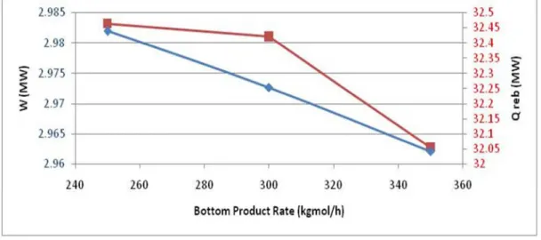
Figure 3-22 - Influence of bottom flow rate on heat load of reboiler and work input to compressor ...28

Figure 4-1 - Schematic diagram of a stage without equilibrium consideration (KOOJIMAN, 1995) ...35

Figure 4-2 - Trays counting (CHOE and JOSEPH ,1984) ...38

Figure 4-3- Flash Tank ...46

Figure 4-4 - EMSOs algorithm for solving DAE ...50

Figure 4-5 - C3 Splitter flow sheet with controllers ...52

Figure 4-6 - Flow rate of stream 4 (kmol/h) ...53

Figure 4-7 - Flow rate of stream 3 (kmol/h) ...53

Figure 4-8 - Level of accumulator ...54

Figure 4-9 - Level of sump ...54

Figure 4-10 - Mole fraction of propylene in stream 4 ...54

(8)

Figure 4-13 - Mole fraction of propane in stream 3 ...55

Figure 4-14 - Liquid flow rate of tray 100 (kmol/h) ...56

Figure 4-15 - Mole fraction of propylene in liquid of tray 100 ...56

Figure 4-16 - Flow rate of stream 1 (t/h) ...58

Figure 4-18 - Mole fraction of propane in stream 1 ...59

Figure 4-23 - Temperature of tray 85 (K) ...60

Figure 4-24 - Temperature of boil up (k) ...61

Figure 4-25 - Temperature of tray 17 (k) ...61

Figure 4-26 - Temperature of tray 171 (k) ...61

(9)

LIST OF TABLES

Table 3-1 - Model details ...12

Table 3-2 - Process specifications for the project case ...21

Table 3-3 - Specification for case_1 (design condition) ...29

Table 3-4 - Comparison for case_1(considering _ErMV=1,_EsMV =1, ηcp= 1) ...30

Table 3-5 - Comparison for case_1 (considering _ErMV=0.7329, _EsMV=0.7592, ηcp= 0.8) ...30

Table 3-6 - Specifications for case_2 (operating condition) ...31

Table 3-7 - Reconciled and plant data ...31

Table 3-8 - Comparison for case_2 (considering _ErMV=1, _EsMV=1, ηcp = 1) ...32

Table 3-9 - Comparison for case_2 (considering _ErMV=0.3, _EsMV=1, ηcp= 0.87) ...32

Table 4-1 - Tuning parameters of controllers ...53

Table 4-2 - Summary of reflux (stream 5) flow rate reduction influence ...57

Table 4-3 - Summary of reboiler inlet (stream 12) reduction influence ...57

Table A-1 - Summary of equations for modeling an adiabatic distillation tray ...73

(10)

NOMENCLATURE

ACRONYMS AND ABBREVIATIONS

EMSO Environment for Modeling, Simulation and Optimization RTO Real Time Optimization

VRD Vapor Recompression Distillation

EO Equation Oriented

DAE Differential-Algebraic Equations ODE Ordinary Differential Equations

SM Sequential Modular

(11)

ROMAN SYMBOL

A

a Tray Active Area

a

Coefficients of Backward Differentiation Formula

B

Steady State Detection Index

B

Bottom flow rate (eq. 4.22)

c

Number of Components

Liquid Total Molar Concentration

Vapor Total Molar Concentration

D

Top Flow rate

d

Series of Data

E

Energy

Transfer Rate Energy per Tray (Liquid Phase)

Transfer Rate Energy per Tray (Vapor Phase)

E

MV Vapor Murphree Efficiency

ƒ

іL Fugacity of Species i (liquid Phase)

ƒ

іV Fugacity of Species i (Vapor Phase)

F

L Feed Flow Rate (liquid Phase)

(12)

G

Parameter (eq. 4.28 and 4.29)

ℎ

Step Size of Backward Differentiation Formula

h

L Liquid Enthalpy

h

V Vapor Enthalpy

hv

Vapor Heat Transfer Coefficient

hl

Liquid Heat Transfer Coefficient

hf

Feed Enthalpy

Diffusive Molar Flux of Component i in the jth Stage (Liquid Phase)

Diffusive molar Flux of Component i in the jth Stage (Vapor Phase)

K

Equilibrium Ratio

k

Controller gain

Binary Mass Transfer Coefficient (Liquid Phase)

Binary Mass Transfer Coefficient (Vapor Phase)

L

Liquid Flow rate

Lagrange Polynomial

L

liq Liquid Level

M

liq

Liquid Molar Hold-up

M

vap

Vapor Molar Hold-up

(13)

N

Number of Trays

n

Degree of Polynomial

η

cp Compressor Efficiency

Molar Transfer Rate of Component i in the Liquid Phase, jth Stage

Molar Transfer Rate of Component i in the Vapor Phase, jth Stage

Total Mass transfer Rate in the jth Stage

NE

Number of Measurements

NY

Number of Variables

P

Pressure

P

L Liquid Pressure

P

V Vapor Pressure

Q

Heat

S

Entropy

T

Temperature

T

L Liquid Temperature

T

V Vapor Temperature

T

s Threshold value

T

w Threshold value

(14)

u

L Liquid Internal Energy

u

V Vapor Internal Energy

V

Vapor Flow rate

V

tray

Tray Volume

ν

L

Specific

Molar volume (Liquid Phase)

ν

V

Specific

Molar volume (Vapor Phase)

X

Differential Variables

x

Mole Fraction of Components (Liquid Phase)

Y

Variable of Data Reconciliation Objective Function

y

Mole Fraction of Components (Vapor Phase)

y

* Vapor Ideal Composition

Z

Algebraic Variables

GREEK SYMBOLS

α

Pressure drop coefficient

α

I

Total Interfacial Area

β

Coefficients of Backward Differentiation Formula

γ

Parameters of Steady State detection Algorithm

∆

P

Pressure Drop

(15)

∆

z

Tray Spacing

θ

Parameters of Steady State detection Algorithm

λ

s

Adjustment Parameter

ξ

Parameters of Steady state detection Algorithm

ρ

Specific Mass

ρ

L Liquid Specific Mass

ρ

V Vapor Specific Mass

σ

2 Variance

Integral time

Ф

_іL Fugacity Coefficient of Species i (Liquid Phase)

Ф

_іV

Fugacity Coefficient of Species i (Vapor Phase)

SUBSCRIPTS AND SUPERSCRIPTS

C

Cold Stream

cp

Compressor

eq

Equilibrium

H

Hot Stream

in

Inlet Stream

L

Liquid Property

(16)

out

Outlet Stream

r

Rectification Zone

re

Reconciled Data

s

Stripping Zone

S

Entropy

sat

Saturated

sub

Subcooled

V

Vapor property

(17)

1. INTRODUCTION

In the chemical process industry, real-time optimization (RTO) is a crucial tool to increase process profitability in scenarios where feedstock composition and market price variations demand rapid adaptation of the process conditions. The benefits achieved from RTO implementation in a process plant depend on the value of increased processing capacity, differences among product prices, specific energy consumption, number of independent variables and constraints, and the ability to accurately model process responses (WHITE, 1997). To date, there are around 300 RTO applications (DARBY et al., 2011) spanning a wide variety of chemical and petrochemical processes (MERCANGOZ; DOYLE, 2008).

The main steps of a classical RTO framework (Figure 1.1) are steady state detection, parameter estimation, and optimization (SEQUEIRA; GRAELLS; PUIGIANER, 2002; NAYSMITH; DOUGLAS, 2008). In the first step, online plant data are analyzed (including data reconciliation and gross error detection) to determine, by some criterion, if the process is (reasonably) steady. Then, the steady state data is used to update some (relevant) parameters of the model such that it can represent the actual plant conditions as closely as possible. In the third step, the updated (adjusted) model is used to optimize the economic objective function, obtaining a new optimal operating point, which becomes the new target for the control system.

Figure 1-1 – Classic RTO

(19)

The success of an RTO strategy largely depends on the mathematical steady state model of the process and its solution. The steady state model must be flexible to adjust the real behavior within a wide interval of process conditions (CHACHUAT et al., 2009) and accurate enough to guarantee that the calculated optimum is close to the real one (KRISHNAN; BARTON; PERKINS, 1992; FORBES; MARLIN; MACGRECOR, 1994). The solution strategy must be able to handle large plant disturbances in a fast and robust way to guarantee a new optimal point at every RTO cycle. These requirements make mechanistic models and equation-oriented (EO) simulation environments especially suitable for RTO applications (MEIXELL; GOCHENOUR; CHEN, 2000; YIP; MARLIN, 2004).

The present work focuses on generating a steady state model suitable to the RTO, and a dynamic model for an industrial-scale C3 splitter column (propane-propylene splitter) owned by Petrobras. The studied C3 splitter column in this work is a vapor recompression distillation (VRD) column which is a system for energy integration systems in process and energy industries. Energy integration is largely used in industry due to the high cost of energy and the corresponding need to minimize utility usage by pairing energy generation and consumption within the same plant. In vapor recompression distillation this energy integration is performed by heating the reboiler with the compressed stream coming from top of the column (NULL HL, 1976).

(20)

affect the outcome of the optimization. The implementation of a rigorous model of the VRD process in an equation-oriented (EO) simulation environment mitigates the convergence difficulties generated by the recycle streams (MEIXELL et al., 2010), which avoids the previously mentioned simplifications and allows a better representation of the process behavior.

In addition to steady state modeling, the present work also considers the development of a dynamic model, which can be applied either as a virtual plant or for Dynamic Real Time Optimization (DRTO).

First proposed methods for solving separation systems models involving tray by tray calculation began in the 30's decade. From the 50's decade, with the advent of digital computers, new algorithms and simulators were developed. In the 70's decade, first commercial simulators were applied in industrial plants and development of rigorous models was considered.

Gani (1986) presented a generic and rigorous dynamic model considering thermodynamic equilibrium between the phases. Hydrodynamic behavior was included with the possibility of the increase of internal liquid and vapor phases and important events such as flooding and tray drying. For proving the efficiency and generality of the model, various industrial simulations were carried out, validating the model with plant data.

(21)

Considering the two latest works, Ruzi (1988) proposed developments of start-up policies for distillation column based on rigorous dynamic simulations. The results of their work led to characterizing the start-up condition of a plant.

Gani (1989) modified the dynamic model in order to use it as a new method for solving steady state simulations. The objective of this work was to obtaining robustness in solving steady state simulations. The exchange between steady state and dynamic models depended on the equations residual. If, with the initial estimates, the set of algebraic equations could not be solved, the problem switched to the dynamic mode. In the dynamic mode, the states were estimated by integration with the initial estimates corresponding to the initial condition. As soon as some integration criteria were achieved, the problem switched to the steady state mode which was solved without major difficulties.

(22)

based on models developed by Gani et al. (1986). The model consisted 266 variables and 97 parameters and was simulated two times faster than real process.

In this work the EMSO environment (Soares et al., 2003) is used, which is able to solve Algebraic and DAE systems. However, rigorous dynamic tray-by-tray modeling of distillation column with the fixed pressure profile leads to high index system of differential and algebraic equations that demands high-order derivatives of thermodynamic properties. As thermodynamic properties calculation are not able to evaluate such derivations, for solving such a system an index one formulation should be proposed. One suggested formulation is adding algebraic equations to the system of equations that determine the vapor and liquid flow rates in the outlet of the trays without fixed pressure profile. Usually for distillation column, this is done by correlating vapor flow to the pressure drop and physical properties of the fluid (Wang et al. 2003), and liquid flow to the liquid level of each tray (Wang et al. 2003). The drawback related to these equations is the uncertainty in the parameters values that involve geometrical characteristics and coefficients, affecting the model response.

Considering that compositions dynamic is much slower compared to flow dynamics and tight pressure control in the case study, the present work proposes a formulation similar to the proportional controller in which for calculating vapor and liquid flow rates the pressure profile and the liquid level are kept approximately constant. The proposed correlations contain the initial condition and only one parameter for each correlation. These parameters are set in order to keep pressure drop and liquid level approximately constant on the trays.

(23)

(24)

2. PROCESS DESCRIPTION

The REPLAN’s Propylene Production Unit was designed to produce 265,000 t/y of propylene polymer grade with high purity (99.5% molar at minimum). The Propylene Production Unit at REPLAN consists of three different distillation towers (Depropanizer, Deethanizer and C3 Splitter). The Unit is fed by the LPG (Liquefied Petroleum Gas) from the FCC Units (Fluid Catalytic Cracking) and produces two product streams: a C4 Cut that is sent to MTBE (Methyl Tertiary Butyl Ether) Unit and Propylene (Figure 2.1).

Figure 2-1- Unit flow sheet

(25)

Figure 2-2 - C3 Splitter flow sheet

Vapor recompression assisted distillation (VRD) is a heat integration technique, widely used in the chemical industry to economically separate close-boiling mixtures, thus its most practical applications occur in binary systems where the separation is difficult (low relative volatility) (HARWARDT; MARQUARDT, 2012; ANNAKOU; MIZSEY, 1995).

The smaller the temperature difference between the top and bottom is, the more profitable the heat pump application will be, for the following reasons: small temperature differences indicate difficult separations with high reflux ratios, and consequently, high steam and cooling water consumptions, and the pressure ratio and the compression power which are required increase with the increase of temperature difference.

(26)

expands through valve and enters the distillation column (DC), where high-purity propylene is obtained as the overhead product, stream 4, and propane is obtained at the bottom, stream 3. The overhead product, mixed with the vapor coming from distribution tank (DT), stream 9, and is compressed to increment its condensing temperature in compressor (CP). One part of the outlet flow from (CP) is sent to condenser (HX1), stream 15, and is used to control column pressure. The rest condenses in reboiler (RB), stream 12. Outlet streams from HX1 and RB, expands through valves V1, V2 respectively, returning to DT where a portion of the liquid is sent to DC as reflux, stream 5, and the other part is sent to storage as main product, stream 4.

Actually, for using conventional distillation column, the operating pressure should be increased so that cooling water can be utilized for condensing the top vapor. However, relative volatility decreases with pressure and separation gets more difficult. By applying Vapor Recompression Distillation (VRD) technology, the column pressure can be kept lower, but the top vapor is compressed in the compressor up to the necessary pressure in such a way that its condensing temperature is greater than the boiling temperature of the column bottom product.

(27)

(28)

3. STEADY STATE MODELI

The steady state model for this process was developed in an Equation Oriented (EO) environment using software EMSO (Environment for Modeling Simulation and Optimization).

In the Sequential Modular approach, unit operations are presented by modules (procedural representation) with defined input and output streams. The output streams are calculated from input streams within each module. When solving a steady state flowsheet, the solution from one module is used as input to the following module in the sequence.

Equation Oriented (EO) modeling is an alternative strategy for solving flowsheet simulations. Instead of solving each block in sequence, EO gathers all the model equations together and solves them at the same time. For the steady state case this is a set of nonlinear algebraic equations (NL), represented by a sparse occurrence matrix with unsymmetric blocks along the diagonal that can be solved by Newton method or other approaches.

The EO strategy can be very effective in the situations where SM struggles, such as:

• highly heat-integrated processes • highly recycled processes

• processes with many specifications • process optimization

Normally, these types of problems are very difficult to solve with SM strategy, because they require many successive solutions to the flowsheet and may contain many nested convergence loops.

(29)

analytical first order derivations. As a result, EO strategy can solve much larger problems using the same computational effort.

The main details of the developed model in this work are given in Appendix A and the model code in EMSO language is available in Appendix D. Table 3.1 represents numerical characteristics of the developed steady state model.

Table 3-1 - Model details

Information Value

Number of Variables 8480

Number of Equations 8463

Number of Specifications 17

Degrees of Freedom 0

The performance of the RTO depends on the plant model accuracy. It should be flexible enough to cover the wide interval of process conditions and accurate enough to guarantee the precision of the optimal point.

Beside this, in this work for initializing the dynamic model, steady state simulation results were applied. More explanations about the dynamic model and necessity of consistent initial conditions can be seen in section 4.3.

(30)

3.1. THERMODYNAMIC EQUILIBRIUM

Thermodynamic equilibrium is provided when thermal, mechanical and chemical conditions are satisfied:

T

L

= T

V (3-1)

P

L

= P

V (3-2)

ƒ

іL

=

ƒ

і V ( i = 1,2,3...c) (3-3)

T is temperature, P is pressure , _ƒ L is the fugacity of the ith component in liquid phase , ƒV is the fugacity of the components in vapor phase, L and V are liquid and vapor molar flow rates respectively.

The fugacity equality is often represented using fugacity coefficient. Fugacity coefficient of component i in the gas solution is defined as:

Ф

_і V

≡

ƒ!

"#$

(i = 1,2,3...c) (3-4)

And for liquid solution:

Ф

_іL

≡

ƒ %

"&$

(i = 1,2,3...c) (3-5)

This allows to write the fugacity equality as follows:

(31)

Propylene-propane mixture shows non-ideal behavior especially in vapor phase due to

high operating pressure

(

MUHLER et al. 1990). Therefore, the dynamic and steady state

modeling of the unit was implemented in EMSO (Environment for Modeling Simulation and Optimization) using PR (Peng-Robinson) equation of state of the VRTHERM thermodynamic package.

Thermodynamic model was selected based on analysis considering different available options. Figure3.1 shows analysis for mixture of propane and propylene at T=293.15K at different pressures in which experimental data was obtained from Ho et al. 2006. As shown, PR equation of state calculates vapor and liquid compositions better comparing to SRK and ASRK.

Figure 3-1 - Thermodynamic models comparison

Besides this, as mass transfer limitations prevent the vapor leaving a tray from being in precise equilibrium within the liquid on the tray; consequently, the assumption of ideal stages is only an approximation. For representing the real situation, Murphree efficiency can be adjusted. Murphree efficiency is the ratio of actual change in the average vapor composition to the change that would occur, if the vapor leaving the tray was in with the liquid leaving the tray.

8 8.5 9 9.5 10 10.5

0 0.2 0.4 0.6 0.8 1

P ( b a r) x,y Propane

Propane-Propylene T=293.15K

(32)

The Murphree vapor phase tray efficiency is the most commonly used efficiency definition, and is the only one with practical importance (eq.(3.7)).

E

іMV

=

#$

()*_+# $$,

#$∗+#$$,

(3-7)

Thus, the worse the contact between the phases of the system, the worse the mass transfer between them and more significant will be the non-idealities inherent in the process, leading to lower values of Murphree efficiency.

3.2. STEADY STATE DETECTION

Steady state detection is an important subject in Real Time Optimization, identification of steady state models, analysis of processes, dada reconciliation and other applications. These applications need data in steady state or close to that, and for this, one efficient technique is necessary.

In this work, steady state detection was applied in order to identify the steady state experimental points. These points were used for evaluating the steady state model and initializing the dynamic model.

There are several approaches for steady state detection. NARASIMHAN et al. (1986) presented the Composite Statistical Test - CST and the Mathematical Test of Evidence -

MTE. In CST, successive time periods are defined and evaluated according to covariance matrix and sample mean, and in MTE, differences in mean value are compared with the variability between periods. CAO and RHINEHART(1995) created a method based on moving average or first order filter.

(33)

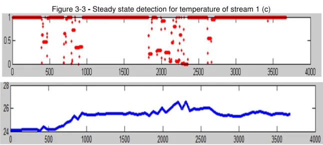
more clarifications on the methodology. Obtained results for some variables of the unit can be seen in Fig (3.2-3.7) in which the first diagram shows steady state index value (Bi(t)) for the variable and the second diagram shows its actual value. Fig (3.8) presents

the results for steady state multivariable index Bm(t).

Figure 3-2 - Steady state detection for flow rate of stream 1 (t/h)

(34)

Figure 3-4 -Steady state detection for flow rate of stream 4 (t/h)

(35)

Figure 3-6 - Steady state detection for flow rate of stream 3 (t/h)

(36)

Figure 3-8 -Steady state detection for the flowsheet

3.3. DATA RECONCILLATION AND PARAMETER ESTIMATION

In order to experimental measurements represent the precise information and reliably describe the process, reconciliation is carried out. Reconciliation is the procedure of fitting the measurements with respect to conservation laws and physical constraints of the system that results in reducing the effect of random errors in the data.

KUEHAN (1961) for the first time presented the data reconciliation in steady state condition. He considered the reconciliation as an optimization problem subject to constraints (mass and energy balances), aiming to minimize the weighted least square objective function:

.

/0

=

∑ ∑

23$4

56₊₃ $4789 :_$49 ;3

<= ;>

<=

(37)

In the above equation, NE is the number of measurements, NY is the number of

variables,

?

@Ais the reconciled variable,

?

Bis the measured variable and σ2 is the

variance of the measured variables.

The weighted least square objective function leads to precise statistics, considering that errors have normal distribution and are not correlated. Beside this, this chosen objective function deals with various set of data, provided that measurement errors are know or that they can be at least estimated. The variance of the measured variables is the normalization factor of variables.

In this work, variables of the objective function (eq. 3.8) are as follows:

• Stream 3 (Bottom product flow rate) • Stream 5 (Reflux flow rate)

• Stream 12 (Reboiler inlet flow rate) • Stream 1 (Feed flow rate)

• Propane concentration in stream 4 (Distillate product) • Propylene concentration in stream 3 (Bottom product)

Besides this, parameters influence on the process response will be analyzed in section 3.4. Estimating the proper value for these parameters is pursued in order to update the model in real time applications.

A simplex optimization routine was applied in both cases for solving data reconciliation and parameter estimation problems in EMSO environment.

3.4. MODEL ANALYSIS

(38)

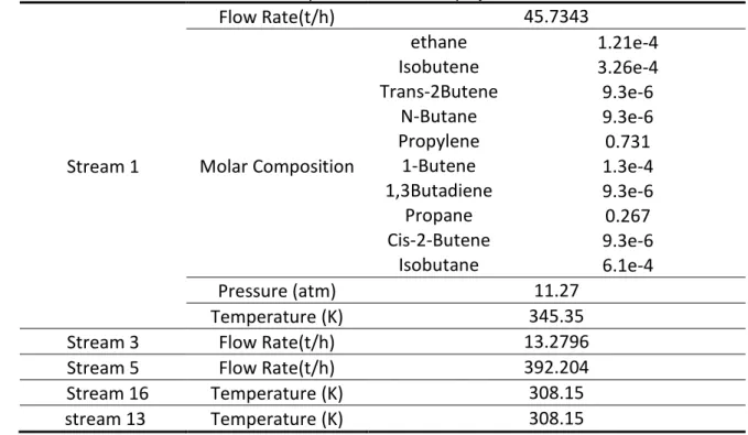
The results shown below correspond to simulations in EMSO with the base specifications presented in Table 3.2.

Table 3-2 - Process specifications for the project case

Stream 1

Flow Rate(t/h) 45.7343

ethane 1.21e-4 Isobutene 3.26e-4 Trans-2Butene 9.3e-6

N-Butane 9.3e-6 Propylene 0.731 Molar Composition 1-Butene 1.3e-4

1,3Butadiene 9.3e-6 Propane 0.267 Cis-2-Butene 9.3e-6

Isobutane 6.1e-4

Pressure (atm) 11.27

Temperature (K) 345.35 Stream 3 Flow Rate(t/h) 13.2796 Stream 5 Flow Rate(t/h) 392.204 Stream 16 Temperature (K) 308.15

stream 13 Temperature (K) 308.15

3.4.1. FEED COMPOSITION

The influence of minor components on the performance of the process is evaluated choosing light (ethane) and heavy (isobutane) components as representatives of this group. The mole fractions of ethane and isobutane in the feed stream were varied in 1 order of magnitude regarding the base case, 1.21×10-4_{_1×10}-3 _{(ethane) and 6.1×10}-4

_6.1×10-3 _{(isobutane); this interval was chosen based on the expected feed composition}

variations in the VRD process at REPLAN.

(39)

Figure 3-9 - Temperature profile for different compositions of Ethane

Figure 3-10 - Temperature profile for different compositions of Isobutane

3.4.2. VAPOR MURPHREE EFFICIENCY

Two vapor Murphree efficiencies, one for the rectification zone (_E_CD! ) and one for the stripping zone (_E_CD!), were defined in order to take into account non-ideality of the mass transfer phenomena in the distillation column.

(40)

Figure 3-11 - Influence of vapor efficiency of rectification zone

Figure 3-12 - Influence of vapor efficiency of stripping zone

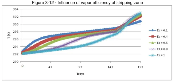
The reduction in mass transfer performance in the rectification zone (low values of ErMV)

causes an increase of the temperatures of the rectification zone and a decrease of the temperatures of the stripping zone. A similar behavior is obtained with respect to the efficiencies of the stripping zone, EsMV.

3.4.3. REFLUX RATIO

(41)

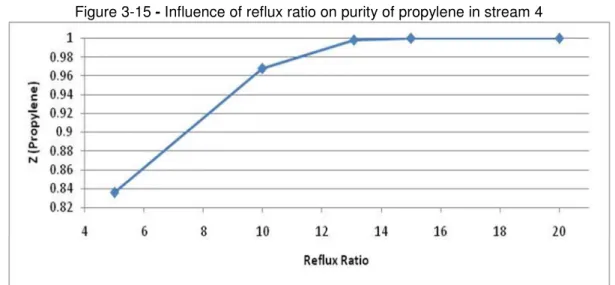
the reflux ratio up to a RR around 12.8, little improvements in purity are achieved for refluxes larger than this value, and the minimum reflux ratio that meets product specifications (mol % of propylene ≥ 99.5 in stream 2) is about 12 (Figure 3.15).

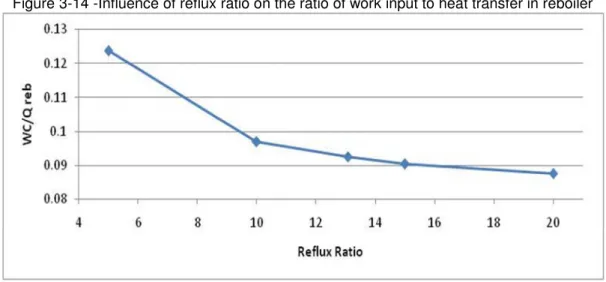
The energy demand of the compressor increases linearly with the reflux ratio (Figure 3.13) and the contribution of the energy supplied to the process by the compressor decreases asymptotically as the reflux ratio increases; this energy represents between 9 and 12% of the heat exchanged in the reboiler (Figure 3.14).

Figure 3-13 -Influence of reflux ratio on work input to the compressor

(42)

Figure 3-15 - Influence of reflux ratio on purity of propylene in stream 4

3.4.4 PRESSURE DROP IN DISTILLATION COLUM

The influence of column pressure drop was evaluated in the interval of 0−1.25 atm, assuming a linear profile, i.e., constant pressure drop per tray. The pressure drop in the distillation column considerably influences the temperature profile of the column (Figure 3.16), especially in the stripping zone. Temperature differences between the first tray and the last tray change from 7.17 K (∆P = 0 atm) to 11.98 K (∆P = 1.25 atm). The heat exchange in the reboiler slightly increases with the pressure drop of the column, 0.2% larger for ∆P = 1.25 atm than when ∆P = 0 atm, while the mole fractions of propylene in tray 1 and propane in tray 197 changed less than 0.1% and 0.5% respectively when compared to the simulation with neglected pressure drop

(43)

Figure 3-17 - Influence of pressure drop on propylene composition profile thought column

3.4.5 COMPRESSOR EFFICIENCY

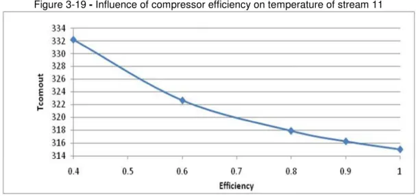
The influence of the isentropic compressor efficiency, ηcp, was analyzed by changing it in the interval 0.4−1. The main changes in the process associated with this variable are in the recycled vapor, stream 8, as well as the outlet temperature and energy consumption in the compressor (Figure 3.18, 3.19). The outlet temperature of the compressor decreases as the efficiency increases; these changes are greater for efficiencies below 0.6. A similar tendency is shown by energy demand.

(44)

Figure 3-19 - Influence of compressor efficiency on temperature of stream 11

3.4.6 BOTTOM FLOW RATE

(45)

Figure 3-20 - Influence of bottom flow rate on mole fraction of propylene in stream 4 and its recovery

Figure 3-21 -Influence of bottom flow rate on flow rate of stream 2

(46)

3.5. VALIDATION OF STEADY STATE MODEL

For inferring the quality of the developed steady state model, validations were performed in two cases. In the first case, validation was carried out considering the process design condition.

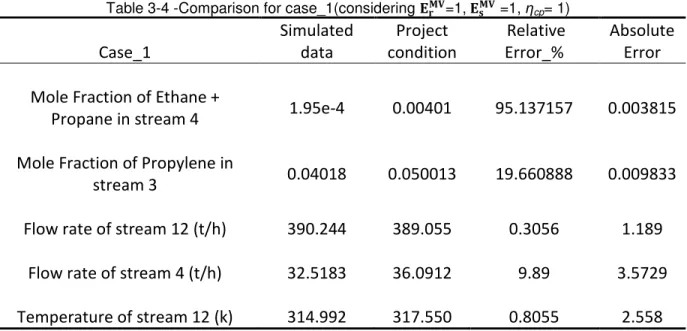
Table 3.3 contains specification for the case 1 (project condition). Table 3.4 shows the simulated data and its relative and absolute error considering Murphree efficiencies of rectification zone, stripping zone and compressor efficiency equal to one.

In order to reproduce bottom and top product specifications and compressor discharge temperature, estimation routine presented in section 3.3 was applied to adjust vapor Murphree efficiency of stripping and rectification zones and compressor efficiency (Table 3.5)

Table 3-3- Specification for case_1 (design condition)

Stream 1

ethane 1.21e-4 Isobutene 3.26e-4 Trans-2Butene 9.3e-6

N-Butane 9.3e-6 Propylene 0.731 Molar Composition 1-Butene 1.3e-4

1,3Butadiene 9.3e-6 Propane 0.267 Cis-2-Butene 9.3e-6

Isobutane 6.1e-4

Temperature (K) 345.35 Stream 3 Flow Rate(t/h) 13.2796 Stream 5 Flow Rate(t/h) 392.204 Stream 16 Temperature (K) 308.15

(47)

Table 3-4 -Comparison for case_1(considering _E_FGH=1,_E_IGH =1, ηcp= 1) Case_1 Simulated data Project condition Relative Error_% Absolute Error

Mole Fraction of Ethane +

Propane in stream 4 1.95e-4 0.00401 95.137157 0.003815

Mole Fraction of Propylene in

stream 3 0.04018 0.050013 19.660888 0.009833

Flow rate of stream 12 (t/h) 390.244 389.055 0.3056 1.189

Flow rate of stream 4 (t/h) 32.5183 36.0912 9.89 3.5729

Temperature of stream 12 (k) 314.992 317.550 0.8055 2.558

Table 3-5 -Comparison for case_1 (considering _E_FGH=0.7329, _E_IGH=0.7592, ηcp= 0.8)

Case_1 Simulated data Project condition Relative Error_% Absolute Error

Mole Fraction of Ethane +

Propane in stream 4 0.004141 0.00401 3.266832918 0.000131

stream 3 0.05037 0.0500133 0.713210286 0.0003567

Flow rate of stream 12 (ton/h) 385.768 389.055 0.8448 3.287

Flow rate of stream 4 (ton/h) 32.5246 36.0912 9.88 3.566

(48)

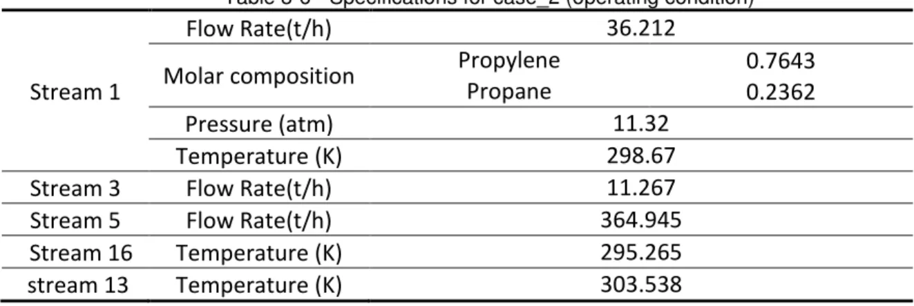
Table 3.7 shows the specifications value before and after reconciliation of data. Table 3.8 illustrates the specifications and simulated results considering Murphree efficiencies of rectification and stripping zones efficiencies and compressor efficiency equal to one. By adjusting the efficiency of both zones and compressor efficiency, top and bottom products specifications and compressor discharge temperature were approached (Table 3.9).

Table 3-6 - Specifications for case_2 (operating condition)

Stream 1

Molar composition Propylene 0.7643

Propane 0.2362

Temperature (K) 298.67

Stream 3 Flow Rate(t/h) 11.267 Stream 5 Flow Rate(t/h) 364.945 Stream 16 Temperature (K) 295.265 stream 13 Temperature (K) 303.538

Table 3-7 - Reconciled and plant data

Plant data Reconciled data

Stream 1 Flow Rate (t/h) 36.212 34.401

(49)

Table 3-8 - Comparison for case_2 (considering _E_CD!=1, _E_JD!=1, ηcp = 1) Case_2 Simulated data Plant Data Relative Error_% Absolute Error Mass Fraction of Propane in

stream 4 1e-7 0.0027 99.996 0.0026999

stream 3 0.2227 0.21438 3.8809 0.00832

Table 3-9 - Comparison for case_2 (considering E_FGH=0.3, E_IGH=1, ηcp= 0.87)

Case_2 Simulated data Plant Data Relative Error_% Absolute Error Mass Fraction of Propane in

stream 4 0.0027 0.0027 0 0

stream 3 0.2291 0.21438 6.8663 0.01472

Mass transfer characteristics in distillation processes are commonly taken into account using vapor Murphree efficiencies. These efficiencies depend on flow regime, tray layout, and physical properties of the mixture (Lockett, 1986).

(50)

(51)

4. DYNAMIC MODEL

Dynamic modeling of distillation column can be carried out applying different approaches involving different levels of complexity in interaction between liquid and vapor and mathematical formulation.

In this chapter, first various types of dynamic modeling approaches are studied. The theory behind these approaches including: complex transfer rate modeling, more simplified models (reduced models) and rigorous models are introduced.

In addition, mathematical issues related to solving higher index system of differential-algebraic equations caused by dynamic modeling of vapor-liquid equilibrium is discussed. Finally, the rigorous tray by tray dynamic model of Vapor Recompression Distillation (VRD) and its validation considering experimental data of plant is presented.

4.1. TRANSFER RATE MODELING

Generally, a stage of a distillation column is modeled with the hypothesis of thermodynamic equilibrium between vapor and liquid, however in reality, this equilibrium is not reachable. The first effort for considering this non-ideality, or non-equilibrium condition, is the efficiency consideration for a equilibrium stage.

To explain the deviation in equilibrium between phases, models based on transfer rates or non-equilibrium models were created. Based on this method, the distillation is modeled by transfer rates that are driven by deviation from the equilibrium and non-equilibrium condition between the phases. In the first works, transfer rates are modeled using Maxwell-Stephan (Maxwell-Stephan models).

(52)

A global schematic representation for a stage, where thermodynamic equilibrium does not exist, can be shown as Figure 4.1.

Figure 4-1 -Schematic diagram of a stage without equilibrium consideration (KOOJIMAN, 1995)

The wavy line in the middle of the diagram represents the interface between phases, that can be liquid and vapor (in the distillation stage case) or two liquid phases (in the extraction case).

These two phases exchange mass and energy with rates N and E. The driving force of

these rates is only due to non-equilibrium consideration between the phases.

Generally, the model of a real stage or the non-equilibrium stage can be divided in three parts. First, the energy and mass balance for the liquid phase, second the balances for the vapor phase, and the third part, interface equations that represent the mass and energy transfer rates and the equilibrium relation.

In mass transfer, liquid and vapor molar rates contain a diffusive (eq.(4.1)) and a convective contribution (eq.(4.2)):

(53)

=

K

L

+

M

(4-2)

=

K

L

+

N

(4-3)

where _KL is the total interfacial area in the stage j and total mass transfer of the

stage j with :

=

∑

O_<= (4-4)

The diffusive flux J, in the matrix form is:

( ) =

[

] (

M − M

L

)

(4-5)

( ) =

[

] (

N

L

− N

)

(4-6)

is the total molar concentration of the vapor phase, is the total molar

concentration of the liquid phase, _Q and _Q are mass transfer coefficients, (M − ML )

and (NL− N ) are the medium difference of the molar fractions between the interface

and the vapor and liquid phase respectively. To calculate these differences, there are many theories and correlations. Generally, these calculations depend on tray geometry and hydraulic conditions.

Similar to the mass transfer, transfer rate of the energy through the interface is written as:

-

= 0

(4-7)

The transfer rate of energy for the liquid and vapor phases is defined as:

=

K

L

ℎR

(

S

-

S

L

) +

∑

O_<=

T

V

(4-8)

(54)

ℎR and _ℎ are convection heat transfer coefficients of the liquid and vapor phases _S , _SL and _S are temperatures of the vapor, interface and liquid and _T is the partial molar enthalpy of the components i in the U V stage.

In addition to mass and energy transfers, the thermodynamic equilibrium through the interface should be considered.

The disadvantage of non-equilibrium model using the transfer rate is the necessity of the mass transfer coefficients matrix which needs experimental data. Unfortunately, this type of data is not easily available in the literature rendering the implementation of this model difficult. Another negative aspect is the necessity of calculating the properties of the additional mixtures, comparing to the equilibrium models. These additional properties are basically the surface tension, viscosity, thermal conductivity, in addition to mass transfer coefficients.

Despite these difficulties, non-equilibrium models can potentially represent distillation systems more accurately than equilibrium models (BIARDI; GROTTOLI, 1989; KOOJIMAN, 1995) but depend on the availability of transfer-related information.

4.2. REDUCED MODELS

(55)

During the decade of 1980, the first principal works about model reduction were published. In that time only integrators for ODE (ordinary differential equations) were available. DAE systems were solved sequentially, thus the simulations were so slow.

Mathematical aspects of dynamic modeling and related index concept will be discussed in more details in the section 4.3.

In 1983, series of works that applied polynomial approximation for model reduction were developed. Orthogonal collocation generally is associated to a technique for discretization of partial differential equations. Using collocation for the simulation of distillation columns is a extension of this technique (HUSS; WESTERBERG, 1996). In the work of CHO and JOSEPH (1984), the procedure for reduction of model variables by orthogonal collocation is presented, providing the basis of the explanation that will be presented in the next paragraph. The procedure of counting the trays for the author is the same as Figure 4.2.

Figure 4-2 -Trays counting (CHOE and JOSEPH ,1984)

(56)

W

X&_X

=

(Lx -Vy)

j-1

- (Lx - Vy)

j j = 1,2,...N (4-10)

Where N is the number of distillation trays. If the concentration profile, x, of a distillation

column could be considered continuous, it could be written as:

x(z)

=

∑

YZ[_<=

N

(4-11)

Where z is the distance along the column, lk(z) are the Lagrange polynomials, xk is the value of x in the arbitrary point z and n is the degree of polynomial.

Writing eq. 4.10 in terms of z:

M

X&

X

| = (Lx - Vy) -

∆

z - (Lx - Vy)

(4-12)

Where ∆z is the tray spacing. n+2 equations are necessary for calculating n+2 xk , 2

corresponds to the boundary condition.

Substituting eq. (4.11) in eq.(4.12), gives :

M

X&4

X

=

∑

YZ[<=

[

- ∆z) -

2 8 ]

(L

N

- V

M

)

j = 2,3, ... n+2 (4-13)

Defining :

^

=

_{2 − _ 8 − 2 8}

(4-14)

Where _^ is the determined constants by the degree of the selected polynomial, eq.(4.15) presents the final form as follows:

M

X&4

X

=

∑

YZ[<=

^

`N − aM

j = 2,3, ... n+2 (4-15)

It should be noted that N balance equations eq.(4.10) were substituted by n reduced

(57)

Choosing a value for n that is much smaller than N, leads to enormous reduction in

order (CHO; JOSEPH, 1984).

This is the basis of polynomial approximation. For reduction of complete model, this procedure should be carried out with the other equations and variables of the rigorous model.

In 1985, Stewart et al. (1985) developed another form of orthogonal collocation where state variables of each stage are approximated by the Hahn polynomial. As the number of collocation points approximates the number of real trays of the system, the response of the reduced system that approximates the response of the complete system gets better with the higher order of approximation allowed by the method (one point of collocation per stage).

STEWARD et al. (1985) and PINTO et al.(1988) tested new strategies for model reduction and analyzed different kinds of orthogonal polynomials. The principal aim of the previous works is the fact that feed tray and the ends of the column (condenser and reboiler) should be considered as the points of collocation and interpolation in order to model reduction gives the best results. Beside this, different orthogonal polynomials than the usual ones (Lagrange, Jacobi and Hahn) were created and applied for the successful model reduction.

BENALLOU et al. (cited MUSCH; STEINER, 1993) proposed one important method of the model reduction based on compartmental models. These models are based on the fact that adjacent trays have small flow rate and temperature differences, so can be considered as a group in “compartments”. Especial energy and mass balances and hydrodynamic relations were developed for these blocks, where only one tray is modeled, that is the reference tray of the block. Various uniform temperature, pressure and flow rates are considered inside the compartments, thus the algebraic equations between the compositions are omitted from each block.

(58)

efficiency and adding components balance differential equations instead of algebraic concentration relations. The principal simplifications of this model, compared to complete rigorous model of distillation column are:

• All of the trays inside a block have the same accumulation;

• The liquid and vapor flow rates inside a compartment are uniform;

• Temperature profile between the adjacent trays until the reference tray is linear;

• Pressure drop of each tray inside a block is equal to pressure drop of the reference tray of the same compartments

Considering theses simplifications, the reduced model contain the following equations:

Per tray:

• (number of components -1 ) differential mass balance equations ;

• (number of components) equations of equilibrium relation between the phases;

Per block (per compartment):

• One global mass balance differential equation; • One energy balance equation;

• One equation for calculating the liquid and one for calculating the vapor flow rate;

• One equation for calculating pressure drop; • One equation of temperature profile interpolation;

The accuracy of model response depends on the number of blocks in which the column was reduced to.

(59)

Additionally, linear low-order models which are obtained from linearizing nonlinear model, are suitable for controller design. Front or wave approach introduced by GILLS and RETZBACH (1980), is not as accurate and general, although it may be useful for some separations.

Many other works with different applications and methodologies were found in the literature, among them, BETLEM (2000) and DIWEKAR et al.(1987) by applying reduced models in batch distillation and a series of works of SIRIVASTAVA and JOSEPH (1985) showed that the degree of model reduction depends on the behavior of temperature profile and presented new methodologies for removing this limitation.

Even thought the reduced models have good precision, for dynamic of system and steady state results, they cannot substitute rigorous models.

4.3. RIGOROUS MODELS

A typical rigorous model of a distillation column consist of equations that describe the components concentration, liquid and vapor flow rates, temperature, pressure drop and the relation between liquid and vapor phases (Appendix C). However, even in this "rigorous" model a number of model simplifications are included. These typically include prefect mixing in both phases on all the trays, thermal and thermodynamic equilibrium between the phases (100% tray efficiency or possibly some simple Murphree relationships for the efficiency of each component).

As for solving steady state modeling, in the dynamic case, there are sequential and modular approaches.

(60)

output of the actual module. For both schemes each module might contain its own integration routine, and the flowsheet calculation might be a combination of explicit and implicit calculations.

When the equation oriented approach is applied to dynamic cases the equation system is a set of ordinary differential and algebraic equations (DAE's), which is usually stiff, sparse and nonlinear. When solving stiff equations, the time step is determined from stability considerations not from accuracy considerations. Hence the ideal integration method for stiff equations is an implicit integration method.

Considering the semi-explicit DAE system as follows:

X´ = f (X,Z,t)

and

g (X,Z,t) = 0

Where:

X- differential variables

Z- algebraic variables

y

T

= [X

T

Z

T

]

It is solved using an extension of ODE solvers. There are two approaches for solving these systems.

1. Nested Approach:

• given

X

n, solve

g (X

n

,Z

n

) = 0

===>

Z

n

(X

n

)

• using ODE method evolve

X

n+1

=

Ф

(X

n

,Z

n

(X

n

),t

n

)

This is the most common approach:

• requires

Z = Z(X)

(implicit function)

• required if only an explicit method is available (e.g. explicit Euler or Runge-Kutta)

(61)

2. Simultaneous Approach (GEAR, 1971):

Solve

X

´

= f (X,Z,t), g(X,Z,t) = 0

simultaneously using an implicit solver to evolve both X and Z in time.

• requires an implicit solver • much more efficient

• provides for more flexible problem specifications

For instance, consider a Backward Differentiation Formula (BDF) solver. For a semi-explicit system, we can write:

X

n+1

= h

β

-1

f (X

n+1

,Z

n+1

,t

n

) +

∑

<c,

K b

Y+

(4-16)

g (X

n+1

, Z

n+1

, t

n+1

) = 0

(4-17)

and this system can be solved for Xn+1, Zn+1 using Newton's method.

ef − ℎg+=

hi

hj −ℎg+= hi hk hl hj hl hk

m n_bYZ=

_oYZ=p = − r

bYZ=s − ∑ b<c Y+t − ℎg+=u bYZ=s , oYZ=s , vYZ=

w bYZ=s , oYZ=s , vYZ= x

(4-18)

Note that the Jacobian matrix is nonsingular at h=0 as long as hl

hy is nonsingular (a

necessary condition for the implicit function Z(X)). Thus if hl

hy is nonsingular, both the

Nested and Simultaneous approaches should work.

The degree of difficulty in solving DAE system depends on the singularity condition of hl_hy

which relates to the system index (PETZOLD, 1982).

For semi-explicit DAE system, the index is the minimum number of times that g(X,Z,t) must be differentiated with respect to time in order to yield a pure ODE system:

X

´

= f (X,Z,t)

(4-19)

(62)

A DAE system of index 1 contains a structurally non-singular subset of algebraic

equations ( hl_hy is nonsingular). Therefore, this can be solved together with the subset of

ODEs or separately at any instant of time, given the initial values of differential variables.

Besides this, as in a DAE with index 1, hl_hy is nonsingular, one can specify X(0) freely

and solve for Z(0) from g(X(0),Z(0),0) = 0. But for high index problems (index > 1), as hl_hy

is singular, X(0) can not be specified freely and we need to analyze and reformulate the DAE to get consistent initial conditions. In particular, consistent initial conditions for such systems must satisfy not only the original equations themselves, but also the first or higher-order differentials with respect to time of some of these equations. Consequently, the number of variables for which arbitrary initial values may be specified is less than the number of differential equations in the system (PANTELIDES, 1988). Soares and Secchi in 2012, studied an alternative approach that can be used to initialize DAE systems. In their work, an algorithm was developed that determines which variables can be specified for both the low and high-index systems so as to obtain a consistent initial values.

For high index DAEs, solvers that are capable of solving this kind of system can be applied or system index can be reduced to one (Index reduction). Index reduction can be implemented manually by adding algebraic equations or algorithms such as Pantelides algorithm and Dummy Derivative algorithm.

Pantelides algorithm determines the equations that must be differentiated in order to make the high-index problem solvable (PANTELIDES, 1988). Dummy Derivative algorithm makes a clever selection of the dummy derivatives in order to obtain a non-singular reduced-order system (MATTASON, 1993).

For showing the index problem and its numerical solution difficulties in our case, a flash tank example is chosen and its index analysis was carried out.

(63)

Figure 4-3- Flash Tank

For a one-component mixture the assumption of vapor-liquid equilibrium gives that the pressure (P) must equal the saturation pressure for the component

P = P

sat

(T)

(4-21)

Consequently, specifying the tank pressure is equivalent to specifying its temperature T.

Furthermore, because Vv is constant, Mvap is directly related to T.

Also in this case considering the "perfect control" assumption, Mliq can be considered as constant. Assume that B (outlet liquid flow) is used to keep the level constant (Mliq). In addition to the feed the independent variables are then D and Q. Given these

independent variables we may obtain the independent variables T (temperature) and B

as functions of time using:

X z{|}

X

= F - B - D

(4-22)

M

Liq X~

• X

+

X z{|}~€

X

= Fh

f

(64)

Many numerical software packages will not be able to solve the mentioned problem. The reason is the "index problem" that arises in general whenever the equations involve differentiation of a variable which is not a state variable. State of a dynamical system is the minimum number of variables that must be specified at t=0 (in addition to the independent variables such as feed, Q and B in this case) in order to be able to solve

the equations for t > 0.

In the present problem there is only one state variable, which may be chosen to be the hold-up Mvap (or equivalently P or T which are directly related to Mvap).

At a given time step the state variable Mvap (and consequently P and T) is known, and the user has to supply the value of Xz_X{|} at this time step.

This derivation is given by eq.(4.22), but first the B, which is an dependent variable,

must be obtained. B may be found from eq.(4.23), but this requires that time derivative of the energy in the tank is known. The term _{•‚ /•v} is approximately equal to _{•ℎ /•v} which appears on the left hand side of eq.(4.23) and may be written as:

XV• X

=

hV• Xz{|}

Xz{|}

X

(4-24)

And we may substitute Xz{|}

X from the material balance and change eq.(4.23) to an

algebraic equation. However, evaluating the term:

hV• Xz{|}

=

XV• X„

(

h„ h"

)

sat h"

hz{|}

(4-25)

requires analytical expression for derivatives of the enthalpy equations, the saturation pressure equation and the equation of state. In general, these may be extremely tedious to obtain, in particular for multicomponent mixtures.